Stacked Autoencoders for Unsupervised
Feature Learning and Multiple Organ Detection
in a Pilot Study Using 4D Patient Data
Hoo-Chang Shin,
Student Member, IEEE,
Matthew R. Orton, David J. Collins, Simon J. Doran,
and Martin O. Leach
Abstract—Medical image analysis remains a challenging application area for artificial intelligence. When applying machine learning, obtaining ground-truth labels for supervised learning is more difficult than in many more common applications of machine learning. This is especially so for datasets with abnormalities, as tissue types and the shapes of the organs in these datasets differ widely. However, organ detection in such an abnormal dataset may have many promising potential real world applications such as automatic diagnosis, automated radiotherapy planning, and medical image retrieval, where new multi-modal medical images provide more information about the imaged tissues for diagnosis. Here we test the application of deep learning methods to organ identification in magnetic resonance medical images, with visual and temporal hierarchical features learnt to categorise object classes from an unlabelled multi-modal DCE-MRI dataset, so that only a weakly supervised training is required for a classifier. A probabilistic patch-based method was employed for multiple organ detection, with the features learnt from the deep learning model. This shows the potential of the deep learning model for application to medical images, despite the difficulty of obtaining libraries of correctly labelled training datasets, and despite the intrinsic abnormalities present in patient datasets.
Index Terms—Edge and feature detection, Object recognition, Pixel classification, Machine learning, Biomedical image processing.
F
1
I
NTRODUCTIONM
EDICAL image analysis remains one of the lessstudied areas of computer vision. Unlike the fre-quently used scene images, for which the features are often well-defined [1]–[3] and where the aim is to recognize an object in a 2D image, medical datasets and the objects contained within them are often 3D, with recognition performed on the component 2D slices. Moreover, while scene images are familiar to us and there are “enough” images with ground-truth provided [4], [5] for the training of machine learning algorithms, medical images are harder to obtain, and the ground-truth labels require substantially more specialist knowl-edge to define. By the same token, the time-consuming nature of the labelling task provides a strong impetus for the development of automated methods, such as those described here. This is especially the case for patient data because of the abnormalities arising from disease. Both the shape and contrast properties of an organ with disease might look significantly different from the corresponding normal tissue. Furthermore, the majority of medical images - including all those containing the pathology that is the likely target and motivation for segmentation studies - are obtained from patients rather than healthy volunteers. This presents significant
prob-• The authors are with the Institute of Cancer Research and Royal Marsden NHS Foundation Trust, Sutton, United Kingdom.
E-mail: {hoo.shin, matthew.orton, david.collins, simon.doran,
mar-tin.leach}@icr.ac.uk
lems in making test datasets widely available, problems which are rooted both in the “data re-use” clauses of the ethical approvals under which a study has been con-ducted, and in the non-disclosure arrangements imposed by the pharmaceutical companies that often sponsor the trials. Multi-modal and so-called “functional” images can provide additional diagnostic information about the tissues being imaged to supplement the standard morphological images. However, the relatively recent introduction of such techniques, together with the cost of the extra imaging, mean that appropriately labelled functional datasets are rare and often available only for small patient cohorts. Dynamic contrast-enhanced magnetic resonance imaging (DCE-MRI) [6] is a typical example: it has become an important tool for cancer diagnosis and assessment of therapeutic outcomes, as it provides information on blood perfusion dynamics and vascular permeability of tissues, but it is uncommon to obtain DCE-MRI from a healthy subject, because there are significant ethical restrictions on the use of contrast agents in non-patients. A 4D DCE-MRI study comprises serial 3D data sets obtained during administration of a contrast agent.
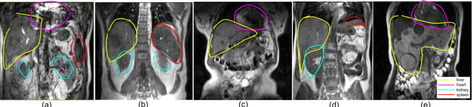
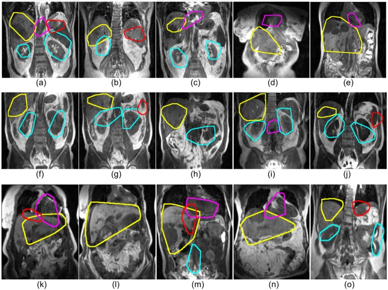
liver heart kidney spleen
liver heart kidney spleen
(a) (b) (c) (d) (e)
Fig. 1:The shapes of the organs vary substantially, and the shape of liver with metastases can be very abnormal (e). Regions were labelled as described in the main text. Note how the exact outline of the organs is not always clear. Uncertainty in identifying the spleen was high, as it is difficult to distinguish from the other nearby organs, for example in (d).
unsupervised, they represent characteristics of the object classes appearing in the dataset, and therefore only “rough guidance” is required from the human operator to train a classifier. Raina et al [8] coined the term “self-taught learning” for this process, and our experiments show that features of the objects can be learnt effectively from unlabelled data, with better representations being learnt when the original data contain richer information from multiple modalities (in this case temporal), rather than simple visual data alone.
Following the approach of [8], we compare our new procedure to Principal Component Analysis (PCA), which serves as a baseline method for unsupervised fea-ture learning and in addition, to a single-convolutional neural network (1-CNN) to demonstrate the effect of pre-training. We also compare our algorithm with two es-tablished feature-learning methods for image and time-series data: Histogram of Oriented Gradients (HOG) [3] and a Discrete Fourier Transform (DFT) approach.
We show that a deep learning with a stacked sparse autoencoder model can be effectively used for unsuper-vised feature learning on a complex dataset for which it is difficult to obtain labelled samples. It makes minimal assumptions about the model describing the given data, and a similar model can be applied to new kinds of dataset with minimal re-design. Previous studies have shown that reducing the number of assumptions about the data and annotations can improve performance on action-classification tasks in multi-modal data [17]. Fur-thermore, an “open” model (i.e., one for which the characteristics of the features learnt can be controlled by its hyper-parameters [9]) can be extended to “context-specific” feature learning. In our case, a typical context is the binary classification of an entity in the dataset as belonging to particular organ class, and this type of learning is an approach in which different sets of features, each set being specific to a given context, can be learned by thesamebase-model. Finally we demonstrate a probabilistic part-based method for object detection, which is used for localization of multiple organs, with the multi-modal features learned from an unlabelled 4D DCE-MRI dataset.
The remainder of the paper is organized as follows: In
Section 2, we review related works in the literature. Sec-tion 3 introduces the 4D patient data used in our study. Section 4 introduces the single-layer sparse autoencoder and reviews a preliminary study of our system applying the sparse autoencoder [10]. The concept of stacked sparse autoencoders, a deep architecture of the single-layer sparse autoencoder applied with max-pooling, is introduced in Section 5, together with analysis and com-parison with other methods. Multi-organ detection with the stacked sparse autoencoders and probabilistic part-based object detection are covered in Section 6, followed by a discussion and conclusion.
2
RELATED
RESEARCH
Our overall aim is to learn the object classes in a min-imally labelled dataset: in other words only a weakly supervised training is required to train a classifier. So called, “part-models” for the self-learning of object classes were studied for 2D images in [11]–[15], in order to achieve object detection in such weakly supervised settings. In our work, a deep network model is used to learn features and part-based object class models in an unsupervised setting.
Deep learning has attracted much interest recently, and has been used in a number of application areas. Many studies have shown how hierarchical structures in images can be learned using deep architectures with application to object recognition [18]–[23]. Object recog-nition and tracking in videos with deep networks was shown in [24], where graphical model was used in addition to unsupervised feature learning by a Restricted Boltzmann Machines (RBM) [25]. Deep neural networks for classification of fMRI brain images was studied in [26], where RBMs were used to classify the stage and action of a volume while the images were taken.
Deep learning of multi-modal features was recently studied in [27]. Our approach is similar, and we use stacked autoencoder model structure for separately learning both visual and temporal features. Independent Subspace Analysis, a deep neural network model for un-supervised multi-modal feature learning was suggested in [28], whereas in [29] and the many previous action-recognition studies appearing in [28], the objective was to recognise the action a video sequence represents. This also applies to [27], where the objective was to use multi-modal feature learning to classify the whole video sequence as a single category. In our study we aim to use unsupervised feature learning to recognise several objects within a given multi-modal dataset.
Previous studies of automated object detection in med-ical images have tended to concentrate on brain images, especially detecting brain tumours. This is largely be-cause both the shape and properties of the brain are more homogeneous across individuals than is the case for other parts of the body; for example, segmentation of MS lesions is reported in [30]–[33]. In all these cases, the disease tends to change the overall shape of the brain relatively little, whereas substantial shape changes can be observed with diseased abdominal organs. Moreover, tumour is not an organ type but is a collection of abnormal tissues, which makes the approach to tumour segmentation different from object detection with a pat-tern recognition approach. Some of the complex tumour types represented by features learnt with a sparse au-toencoder in our dataset can be seen later in Section 4.1 and Figure 4. In previous work [34], we suggested an approach for brain tumour segmentation, in which a single-layer sparse autoencoder was used to learn the features present in the variation of image brightness in multi-parametric MR images, followed by spatial clustering and logistic regression to segment oedema and tumour. Whilst this result indicates the potential of applying sparse autoencoders for medical image classi-fication, the methods in [34] require additional elements to enable abdominal organ detection and classification to be performed at the same time.
The abdominal region contains many important or-gans and therefore, has great potential to be useful for automated diagnosis and radiotherapy planning. Multi-organ detection was demonstrated in computed tomography (CT) images in [35], in contrast-enhanced
abdominal CT images in [36], and in whole-body MR Dixon sequences in [37]. In all of these cases a clearly labelled training dataset was required. Multi-organ seg-mentation on CT images using active learning with a minimal supervisory training set was demonstrated in [38], although in this study, a clinical expert’s presence was required for the consecutive labelling during the active learning process. Also, the organs in the dataset in the studies are not largely abnormal as is the case in our data with tumors.
To our knowledge, there has not yet been an appli-cation of unsupervised feature learning with a deep learning approach to object recognition in medical im-ages with large heterogeneous datasets. We demonstrate multi-organ detection in 4D DCE-MRI patient data, us-ing the hierarchical multi-modal features learned from an unlabelled subset of datasets with 78 patient scans.
The training, cross-validation and test dataset are anonymised patient data from different studies of dis-eases, and our results show that the proposed method successfully learns features that lead to good classifica-tion performance in complex and variable datasets with low image resolution and noisy ground thruth labels.
3
D
ATASETOur 4D dataset consists of a time series of 3D DCE-MRI scans from two studies of liver metastases and one study of kidney metastases:
• Dataset A: 46 scans of patients with liver metastases,
each containing 7-12 contiguous coronal slices with image size256×256, repeated atT = 40time points
• Dataset B: 3 scans of patients with kidney
metas-tases, each containing 14 contiguous coronal slices with size256×267, repeated at T = 40time points
• Dataset C: 29 scans of patients with liver metastases
from a clinical trial, each containing 14 contiguous coronal slices with image size209×256, repeated at
T = 40time points.
x=256
z=2
56 …
t=1
… …
t=13 t=40
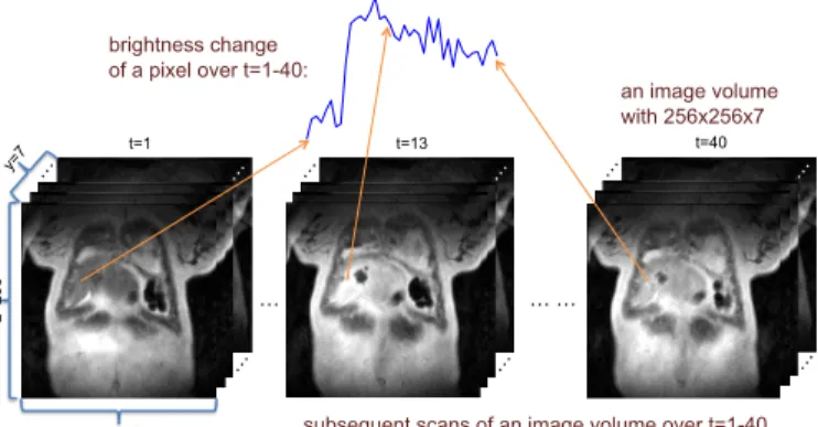
brightness change of a pixel over t=1-40:
an image volume with 256x256x7
subsequent scans of an image volume over t=1-40
Fig. 2:A 4D DCE-MRI scan of a liver patient for a time course 1≤t≤40with volume size of256×256×7. Each pixel of an image slice in a volume gives a time series of its brightness over 40 images. The time series represents the perfusion status of the tissue in the voxel and will vary with tissue types.
the successive images changes according to the blood perfusion dynamics and vascular permeability of the tissues observed. DCE-MRI images of a liver patient scan and a time series of a liver voxels brightness change are shown in Figure 2.
Subsets of Dataset A were used for training, subsets of Dataset B for cross-validation, and Dataset C was used for the final visualization and test, respectively. “Rough” outlines encompassing the labelled tissues, as shown in Figure 1, were drawn by a non-expert, and subsequently adjusted and confirmed by a radiologist. These outlines are used for supervised training in the training dataset, and performance evaluation in the cross-validation dataset.
4
S
INGLE-
LAYERS
PARSEA
UTOENCODERAn autoencoder is a symmetrical neural network to learn the features of a dataset in an unsupervised manner. This is done by minimizing the reconstruction error between the input data at the encoding layer and its reconstruc-tion at the decoding layer, so that the correlareconstruc-tion between the input features are learned in an EM-like fashion [19], [40] in the mapping weight vectors.
Encoding of an input vector x ∈ RD×1 is done by
applying a linear mapping and a nonlinear activation function to the network:
a=sigm(Wx+b1), (1)
where W ∈RN×D is a weight matrix withN features,
b1∈RN is an encoding bias, andsigm(x)is the logistic sigmoid function (1 + exp(−x))−1. Decoding of a is
performed using a separate decoding matrix:
z=VTa+b2, (2)
where b2 is a decoding bias and the decoding matrix
is V ∈ RN×D. Features in the data are learned by minimizing the reconstruction error of the likelihood function L(X,Z) = 1
2
Pm
i=1||zi−xi||22, where X and Z
are all the training and reconstructed data respectively, and the features are encapsulated in W.
While an autoencoder has a close relationship to PCA by usually performing a dimensionality reduction, an “overcomplete” (larger than the input dimension) non-linear mapping of the input vector x can be made by applying sparsity to the target activation function, that is, a sparse autoencoder [41]–[45]. To achieve this, the ob-jective in the sparse autoencoder learning is to minimize the reconstruction error with a sparsity constraint:
L(X,Z) +β
N
X
j=1
KL(ρ||ρˆj) (3)
where β is the weight of the sparsity penalty, N is the number of features in the weight matrix, ρis the target average activation of a and ρˆj = m1 P
m
i=1[aj]i is the average activation of jth input vector aj over the m training data. The Kullback-Leibler divergence [46] is given by:
KL(ρ||ρˆj) =ρlog
ρ ˆ ρj
+ (1−ρ)log1−ρ 1−ρˆj
(4)
which provides the sparsity constraint – a non-redundant overcomplete feature set will be learned when
ρis small, as in sparse coding [47].
The model is trained by optimizing the objective func-tion (Equafunc-tion 3) with respect to W, V, b1 and b2,
where we used backpropagation [48] and L-BFGS [49] to train the model. It is generally accepted that classification performance is improved by increasing the number of learned features (N), and the effect of the number of features on classification performance using single-layer networks has been studied in more detail in [50].
Our DCE-MRI data have both temporal and spatial domains. Temporal features are learnt from the organ-specific changes in intensity that occur over time, as the contrast agent is differentially absorbed. Following the intensity of each 3D voxel in a set ofny coronal slices of matrix sizenx×nzthroughT time-points provides a set ofnxnynzvoxel “contrast uptake curves”. Features in the spatial domain are identified in our work by sampling 2D image “patches” as described below.
4.1 Application of single-layer sparse autoencoders to temporal feature learning
Approximately 1.3×10⁴ time series signals were
Student Version of MATLAB
Student Version of MATLAB
(a) (b)
Fig. 3:256 overcomplete (a) temporal and (b)8×8size visual feature set learned by unsupervised sparse feature learning.
the individual weightswj∈R40×1 (rows) of the weight matrixW∈RN×40.
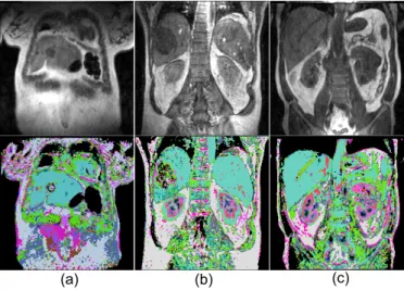
Certain vascular characteristics of a tissue can be represented by its time series in the 4D DCE-MRI image dataset, so that the temporal features alone may be sufficient for unsupervised tissue type classification. Un-supervised tissue type classification using a single-layer sparse autoencoder was evaluated and visualization was previously reported [10]. In this work, we(1)performed dimensionality reduction in the temporal space with a single layer autoencoder network, (2)did vector quanti-zation of the features with a sigmoid activation function, and(3)mapped the result of the vector quantization into RGB space. Three examples of these results are shown in Figure 4.
(a) (b) (c)
Fig. 4: Visualization of dimensionality reduction with a single-layer sparse autoencoder, where the size of the DCE-MRI temporal dimension is reduced from 40 to 16 elements. Different tissue types are visualized in different colors, and a liver tumor is represented as a complex pattern within liver (a), (b). Ambigu-ities in identifying some tissue types of different organs remain, with some sub-regions of the aorta, heart, liver and spleen being represented as the same cyan color.
Different tissue types are represented in different col-ors - liver in cyan and blood vessels in green. Heart and kidney are represented as a number of different colors,
but the color pattern is consistent. Liver tumors appear as a complex pattern of different classes. With this method some tissues of different organs appear labelled as being of the same class, for example liver, spleen and part of the heart and aorta all appear as the same cyan color. This approach does not use the spatial information in the data, so although an organ with more constant tissue characteristic can be detected and segmented, an organ which consists of a combination of different tissue types is not detected as a single entity. Our aim here is to solve these problems by using deep architectures with spatial-pooling so that feature learning can incorporate progressively larger spatial regions.
4.2 Application of single-layer sparse autoencoders to visual feature learning
There are many existing reports on the application of deep learning to classification using the purely spatial features found in 2D images. We describe these as “vi-sual features”, in order to have a clear distinction from temporal features with spatial pooling (see Section 5). In later sections we compare visual and temporal fea-tures separately, and shallow combined representation of multi-modal features [27], as an augmented input to an organ classifier. We learnt 2D visual features from approximately 1.3×10⁴ image patches randomly
sam-pled from the first image slice in each time-series (before the contrast agent is injected), also excluding patches containing background or voxels affected by breathing motion. For image patches of size m ×m the visual features learnt by the autoencoder are given by weight vectorswj ∈Rm
2×1
and N vectors combine to give the weight matrixW∈RN×m
2
.
Temporal and visual features for our data are shown in Figure 3. They represent an overcomplete set of 256 temporal features, and there is no obvious redundancy or repetition of trivial signals (Figure 3 (a)). The visual bases in Figure 3 (b) are learnt from8×8image patches and show Gabor-like edge detectors of different orienta-tions and locaorienta-tions, which are coherent with the results of the previous studies [9], [41]. We apply these features of different input modalities to build a part-based model for multiple organ detection (see Section 6).
5
S
TACKEDS
PARSEA
UTOENCODERSStacked sparse autoencoders – a deep learning archi-tecture of sparse autoencoders – are built by stacking additional unsupervised feature learning layers, and can be trained using greedy methods for each additional layer [42]. By applying a pooling operation [18], [52] after each layer, features of progressively larger input regions are essentially compressed, and this approach is used to build a part-based model for multiple organ detection.
images in [11]–[15], and for action recognition in video sequences in [17], where in [17] the parts were called the “interest-points”. The visual feature learning layer already captures a certain spatial region (patch), which could then correspond to a part of an organ. But the temporal feature learning layer captures only a pixel in the spatial domain, and so a larger spatial proximity of temporal features (e.g. a part of an organ represented by temporal features) is captured by applying max-pooling:
y=max{|Wx1,Wx2, ...,WxR|}, (5)
whereWis the encoding matrix (distinct for each layer), x1, ...,xR are the input vectors to the max-pooling oper-ation and the max and modulus functions are applied element-wise. For the application of max-pooling after the temporal feature learning layer, W is the temporal feature set andxiis a time-series signal. For max-pooling on an M×M patch,R=M2.
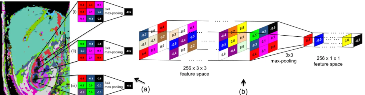
As an example, a conceptual visualization of3×3 max-pooling for3×3size patches in a 2D feature space using the visualization of Figure 4 (c) is shown in Figure 5 (a), and for a 3×3 patch in 3D temporal feature space is visualized in Figure 5 (b). It can be seen how the patches located on different regions of kidney can capture the same temporal feature from a given patch size.
Features of next level spatial hierarchy – object parts with larger region of spatial invariant feature set – are captured by a successive unsupervised feature learning on the max-pooled ouput of the features to learn the features of larger input region, based on what it has learnt for a smaller input region. We examine in the following sections whether useful features are learnt in the second feature learning layer. Examples of our model of two-layer stacked sparse autoencoder networks for learning hierarchical visual features and temporal features, each with a classifier network as the final layer, are shown in Figure 6. Max-pooling in the visual feature learning network is applied such that each layer captures the same size of 2D spatial area as the temporal feature learning layer.
This can be compared with the “bag-of-words” model for image classification [53], [54], where the application of convolutional unsupervised feature learning for the learning of successive layers is conceptually similar to the spatial pyramid matching model [15], [55]. In our case, we are dealing with a “bag of spatial & temporal words”. Some of the differences of the stacked sparse-autoencoder approach in this study to the works cited are that: (1) spatial & temporal features are used in our work as opposed to visual features only such as SIFT [1] and HOG [3], (2) orientation of the features is pre-defined in [15], (3)next-level features with the previous hierarchy features as priors are learnt in the successive autoencoder learning, whereas the same feature is used for all of the spatial pyramid hierarchies.
We compare our unsupervised learning method using sparse autoencoders with more popular, pre-defined
fea-tures for vision and time-series: HOG and DFT. We also compare PCA as a baseline method for unsupervised feature learning, and as well see whether PCA can be applied to successive hierarchical feature learning.
5.2 Analysis and Comparison with Other Methods
The extent to which the learned features can represent our object classes is evaluated by the patch-wise classifi-cation accuracy of organs, based on the labels obtained from the roughly drawn regions of interest (ROIs) as shown in Figure 1. Since the labeled regions include voxels from outside the intended organ, the accuracy cannot be 100%, even with perfect classification. How-ever, as the labeled regions contain more correct voxels than incorrect voxels, we assume that higher accuracy corresponds to a better classification performance.
We compare our unsupervised feature learning meth-ods using stacked autoencoders (SAE) to PCA, as PCA is a popular unsupervised feature learning method. We also evaluate whether PCA can learn hierarchical features when applied successively with max-pooling, where we use 16 principal components for projection of the input data. We test SAE with both 16 (SAE-16) and 256 (SAE-256) learned features to make a fair comparison with PCA using 16 features, and to see the effect of the number of SAE learned features and overcompleteness on classification performance.
A single layer convolutional network (1-CNN) is also tested to see the effect of pre-training on the features, and in addition, a single convolutional network using HOG visual features and DFT temporal features. Clas-sification is done with a single-layer classifier network, where the parameters for the training are chosen by a cross-validation test on small subsets of the data. With the best parameters so derived, the final accuracy is reported after additional training and cross-validation using larger subsets of the dataset. Unsupervised feature learning and classifier training uses only dataset A, and classification is performed only with dataset B, to show the applicability of the features learned unsupervised to an unseen dataset.
Deep networks are known to be difficult to train, and this certainly applies to stacked sparse autoencoder training where there are many hyper-parameters affect-ing the behaviour of the model. The hyper-parameters required for training the sparse autoencoders are the target mean activation ρ, the weight of the sparsity penaltyβ, and the weight decay for the backpropagation optimizationλ. We used a coordinate-ascent-like method to optimise these for each layer, together with the patch and pooling sizes. Coordinate ascent consists of opti-mising each parameter while the others are fixed, and repeating this process for a certain number of iterations until the performance converges.
(a) (b) 0.4 0.4 0.1
0.4 0.1 -0.3
0.1 -0.3 -0.6
-0.6 3x3 max-pooling
0.5 -0.3 -0.6
-0.3 0.1 0.1
0.4 0.1 0.4
0.4 -0.3 -0.6
0.5 0.5 -0.3
-0.2 0.5 -0.3
-0.6 3x3 max-pooling (i)
(ii)
(iii) 3x3 max-pooling -0.6
… … … …
… … … …
256 x 3 x 3 feature space
3x3
max-pooling feature space 256 x 1 x 1
… … … … … … … … … … … …
Fig. 5:(a) A conceptual visualization of max-pooling on a 2D feature space, showing how it can capture the same feature for the patches at different locations in the kidney in Figure 4 (c). (b) A conceptual visualization of3×3max-pooling on a 3D temporal feature space with 256 temporal features.
…
…
…
…
…
…
…
256x256 image 8x8 image patch1st hidden layer with 256 nodes
256x11x11 visual feature space (2nd hierarchy) input layer
with 64 nodes
2nd hidden layer with 256 nodes
1st hidden layer with 256 nodes
2nd hidden layer with 256 nodes 40x256x256
time series volume
256x256x256 temporal feature space (1st hierarchy)
8x8 max-pooling
256x32x32 temporal feature space (1st hierarchy)
…
3rd hidden layer with 256 nodes
3rd hidden layer with 256 nodes 256x32x32
visual feature space (1st hierarchy)
256x32x32 temporal feature space (2nd hierarchy)
256x11x11 temporal feature space (2nd hierarchy) 3x3 max- pooling 3x3 max- pooling liver heart kidney spleen not-of-interest
256x8x8 1st hierarchy temporal feature volume patch
… … … … … … … … … … … … … … … … … … … … … … … … … … … … … … … … … … … … … … … … … … … … … … … … … … … … … … … … … liver heart kidney spleen not-of-interest input layer with 40 nodes
256x3x3 2nd hierarchy temporal feature volume patch 256x3x3 1st
hierarchy visual feature volume patch
… … … … … … … … … 256x11x11 visual feature space (1st hierarchy)
Fig. 6:The overall architecture of the visual feature learning networks (top) and temporal feature extraction networks (bottom). The first and second hidden layers are unsupervised feature learning networks, and the third hidden layer is a classification network, which is trained with supervision to classify patches of different organs.
hyper-parameters, and patch-/pooling- sizes. During the optimization process, the classification performance of each individual object class is recorded as well, but in F1-score rather than in accuracy because in this case the true/false label is biased for each class to the others, where F1-score is defined as F1 = 2 · precisionprecision+·recallrecall, and precision=tp/(tp+f p), recall=tp/(tp+f n), tp: true positives, f p: false positives, f n: false negatives. The averaged F1-score F1avg over each class’s F1-score for
the optimal overall classification accuracy and the corre-sponding hyper-parameter settings are shown in Table 1 as well, and will be discussed later in Section 5.4.
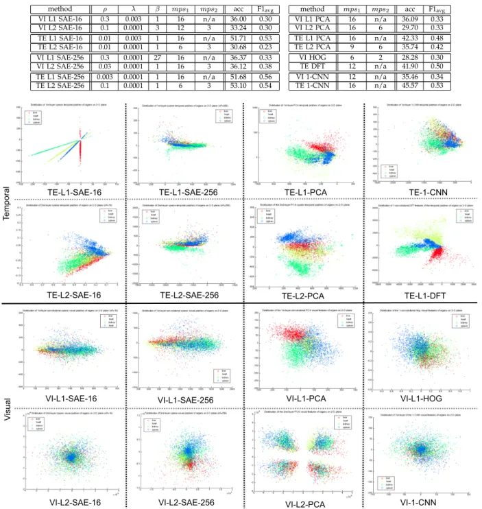
TABLE 1:Part-based classification accuracies and the stacked sparse autoencoder (SAE) hyper-parameters (including patch and pooling sizes) used with: first and second level hierarchy (L1 and L2); visual and temporal features (VI and TE); 16 and 256 learned features. Baseline models are compared with their average classification accuracies for organs (acc), and average F1-score (F1avg)
of each individual object class’s score is shown for comparison later in Section 5.4 with Table 2.
method ρ λ β mps1 mps2 acc F1avg
VI L1 SAE-16 0.3 0.003 1 16 n/a 36.00 0.30
VI L2 SAE-16 0.1 0.0001 3 12 3 33.24 0.30
TE L1 SAE-16 0.01 0.003 1 16 n/a 51.71 0.53
TE L2 SAE-16 0.01 0.0001 1 6 3 30.68 0.23
VI L1 SAE-256 0.3 0.0001 27 16 n/a 36.37 0.33
VI L2 SAE-256 0.03 0.0001 1 16 3 36.12 0.38
TE L1 SAE-256 0.003 0.0001 1 16 n/a 51.68 0.56
TE L2 SAE-256 0.1 0.0001 1 6 3 53.10 0.54
method mps1 mps2 acc F1avg
VI L1 PCA 16 n/a 36.09 0.33
VI L2 PCA 16 6 29.70 0.33
TE L1 PCA 16 n/a 42.33 0.48
TE L2 PCA 9 6 35.74 0.42
VI HOG 6 2 28.28 0.30
TE DFT 12 n/a 41.90 0.50
VI 1-CNN 12 n/a 35.46 0.34
TE 1-CNN 16 n/a 45.57 0.53
TE-L1-SAE-16 TE-L1-PCA
TE-L1-DFT TE-1-CNN
Te
mp
ora
l
V
isu
al
VI-1-CNN TE-L2-SAE-16
TE-L1-SAE-256
VI-L2-SAE-16 VI-L2-PCA TE-L2-SAE-256
VI-L2-SAE-256
VI-L1-SAE-16 VI-L1-SAE-256 VI-L1-PCA VI-L1-HOG TE-L2-PCA
Fig. 7:Scatter plots showing 1500 randomly sampled patches of the organ object classes (red: liver, yellow: heart, green: kidney, blue: spleen) in the training dataset with each of the feature learning methods, and projected onto 2D space using PCA.
5.3 Unsupervised Learning of Object Classes
Patches of organ classes filtered with each of the feature compared are shown in Figure 7 as 2D scatter plots. From the training dataset, 1500 patches are sampled randomly for each organ category, filtered with the features, and the dimension of the patches is reduced to two using PCA in order to aid visualization. It is noticeable that the object classes are very well captured by the 16 temporal features learned by single layer
Student Version of MATLAB Student Version of MATLAB
Student Version of MATLAB Student Version of MATLAB
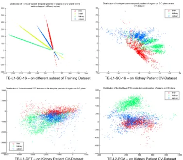
TE-L1-SC-16 – on different subset of Training Dataset TE-L1-SC-16 – on Kidney Patient CV-Dataset
TE-L1-DFT – on Kidney Patient CV-Dataset TE-L2-PCA – on Kidney Patient CV-Dataset
Te
mp
ora
l
Fig. 8:Scatter plots showing 1500 randomly sampled patches of a different subset of the training dataset and the cross-validation liver patient dataset. The patches are processed and displayed in the same way as for Figure 7. Since the scans of the cross-validation dataset are focused on the kidneys, heart does not appear in those images due to its anatomical location, therefore heart is absent in the cross-validation dataset.
This is due to the dramatic dimensionality reduction needed for visualization (256 to 2), as the classification performance with those features show good results in Table 1. Overall, temporal features have better classifica-tion performance than visual-only features.
Figure 7 appears to show nearly perfect categorisation of self-learned features for the TE-L1-SC-16 approach, but the reason the classification accuracy is not higher than that in Table 1 can be seen in Figure 8. Figure 8 shows 1500 randomly sampled patches of a new subset of the training dataset (liver patient dataset) and cross-validation dataset (kidney patient dataset), each filtered with the same temporal features used in Figure 7. Although the TE-L1-SAE-16 features separate the organ classes very well in the new subset of the training dataset, the separation is not nearly as clear on the cross-validation dataset. This performance reduction could be mitigated by unsupervised feature learning on a larger subset of (more heterogeneous) training data, but it is technically challenging to train on a very large scale dataset. In Figure 8 patches of the cross-validation dataset filtered with TE-L1-DFT and TE-L2-PCA - which showed good separation of the organ classes with the training data - are also shown, and they too show less clear separation in the cross-validation dataset.
5.4 Context-Specific Feature Learning
Different organ classes have different properties, and therefore it seems reasonable to suppose that the task of separating a given organ class from all other classes might be best achieved by learning the optimal feature
for that particular organ, rather than by training on the average separation performance for all classes. Applying this in the context of action recognition as in [17] the question would be: Can one obtain better performance with a feature learning model optimized specifically for “hand waving”, for example, rather than using the same feature learning model that simultaneously tries to classify, say, “running” and all the other different actions studied?
It is normally time-consuming and difficult to design a new feature-learning model for every object class, but deep learning requires very little modification. In our study, we applied a model with the same basic design for both visual and temporal feature learning. Moreover, features of different characteristics can be learned by tuning the hyper-parameters in the learning model, as was studied in [9].
In principle one would optimize the hyper-parameters in Table 1 separately for each object class, but the com-putational resource required to do this exceeded what was available for this study. Instead, during the hyper-parameter optimization process in Section 5.2 and Table 1, we picked parameter sets with the best F1-scores of each object class along the trajectory of optimization process. The best F1-scores for each object class along the optimization process of overall classification accuracies in Table 1 are shown in Table 2 as F1tmp, with their
corresponding hyper-parameter sets.
We then train one-vs-all classifiers by logistic regres-sion using the parameter sets with the same inputs as the multi-class classifier from the convolutional network. The one-vs-all classification accuracies with equal num-ber of true/false labels, optimised for each object class is shown as accopt in Table 2. For the results using
visual and temporal features only, the accuracy with first autoencoder layer is denoted by accl+/-if accoptwas
achieved by second autoencoder layer, whereas accl
+/-represents the accuracy with second autoencoder layer if the accopt was achieved by first autoencoder layer.
A shallow combined representation of multi-modal fea-tures [27] is examined as well for both hierarchy autoen-coders, and their classification accuracies both with first (accl1) and second (accl2) autoencoder layers are shown
in the right-hand section of the table. The final classi-fier networks with the context-specific feature learning model for each object class is shown in Figure 9.
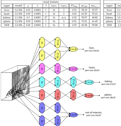
TABLE 2:Model and hyper-parameters of visual and temporal features for each organ class for the context-specific feature learning. The classification accuracy with the chosen model for each organ classaccoptis shown for the cross-validation dataset for all organs
except for heart (which does not appear in the cross-validation data and so is tested on a subset of training dataset). Accuracy with higher/lower autoencoder layer (accl+/-) is compared with that of the first/second layer giving the optimal accuracy (accopt). The
average F1-score in picking the parameters in the optimization process in Table 1 is also shown:F1tmp. (NOI = Not of interest)
visual features
organ model ρ λ β mps1 mps2 F1tmp accopt acc
l+/-liver L2-256 0.03 0.0001 1 16 3 0.53 58.10 52.57
heart L2-256 0.03 0.0001 1 16 3 0.43 63.25 55.23
kidney L1-256 0.3 0.0001 27 16 n/a 0.32 52.97 49.82
spleen L2-256 0.03 0.0001 1 16 3 0.51 73.21 61.45
NOI L2-256 0.03 0.0001 1 16 3 0.35 60.38 59.88
temporal features
organ model ρ λ β mps1 mps2 F1tmp accopt acc
l+/-liver L1-256 0.3 0.0001 27 16 n/a 0.50 64.78 57.46
heart L1-256 0.3 0.0001 1 16 n/a 0.81 84.88 84.54
kidney L2-256 0.3 0.0001 1 9 3 0.72 81.82 79.16
spleen L2-256 0.01 0.0001 1 6 3 0.54 78.44 73.13
NOI L1-16 0.3 0.0001 1 8 3 0.58 58.09 52.01
combined
organ accl1 accl2
liver 66.80 62.62
heart 68.35 65.59
kidney 68.28 79.41
spleen 66.97 63.44
NOI 70.61 62.01
Student Version of MATLAB Student Version of MATLAB
Student Version of MATLAB
TE&
VI&
TE&
TE&
TE&
VI&
TE&
TECL1
&
VIC
L1
&
TECL1
&
TECL1
&
TECL1
&
TECL1
&
VIC
L1
&
TECL2
&
TECL2
&
1CvsCall&
1CvsCall& 1CvsCall& 1CvsCall&
1CvsCall&
kidney,&
partCsize:27x27&
spleen,&
partCsize:18x18&&
liver,&
partCsize:16x16&&
heart,&
partCsize:16x16&
notCofCinterest,&
partCsize:16x16&&
Fig. 9: A conceptual visualization of the usage of context-specific features with stacked autoencoders in classification. Patches of different modalities are sampled from the dataset and go through different feature networks to be classified as an object part of an organ category.
larger region (e.g.48×48) than the second-level temporal features (e.g. 24×24).(4)Shallow combination of visual and temporal features showed better performance than features of either modality alone for liver and “not-of-interest” (NOI) tissues, although the increase in accuracy for liver was small.
It is also possible to draw some conclusions from these results about the parameter settings for deep network models with stacked autoencoders: (1) The optimized sparsity ρ in the second layer tends to be lower than that in the first layer to capture fewer and larger size higher hierarchy features. (2) The weight decay λ and regularizationβ affect the behaviour of the autoencoder less than the sparsity parameter ρ. (3) In the temporal domain, a larger feature set (256) was selected for organs, than for NOI tissues (16 features) - this is probably because NOI does not represent a specific object class, and so the fewer features are used, the less prone is the model to overfitting specific background entities in the training data.
6
PART-BASED
MULTI-ORGAN
DETECTION
From the results in Table 2, we chose: TE-L1-256 features for heart, TE-L2-256 for kidney and spleen, the combined
L1-16 features for NOI and the combined L1-256 features for liver. Some of the part-based organ detection results in training, cross-validation (CV), and the test dataset are shown in Figure 10. As might be expected, the results reflect the organs at which the image datasets themselves were targeted. Thus, liver is better recognized on the scans whose purpose was to image liver tumours, and kidney in renal cell carcinoma patients.
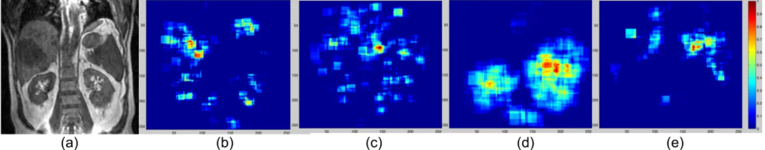
6.1 Probabilistic Part-based Organ Detection As more patches are classified correctly than incorrectly to their corresponding category of organ, we perform probabilistic part-based organ detection, first by gener-ating a probability map for each organ, and then by selecting a threshold to generate a binary mask, using the features selected in Table 2. The probability map is generated using 1000 randomly sampled patches, where the sampling location is on the non-background regions and the regions not affected by the breathing motion. Consider the probability map for organ A. We iterate through all patches and for each pixel location (i, j)of the map, we increase its score for being an organA by 1 unit if the location (i, j)is in a patch classified as the organA. On the other hand, if(i, j)is in the patch but the classifier returns a different class, we subtract 0.2 from the score. The final scores after all patches have been considered is normalized by dividing by the maximum score in the image. The importance of including the NOI class in all our analyses is thus clear. An example of a probability map is shown in Figure 11.
(c) (d) (e) (f)
(a) (b)
Fig. 10:Classification results of part-based organ detection (yellow: liver, magenta: heart, cyan: kidney, red: spleen, blue: not-of-interest (NOI)). (a,b): liver patient training dataset, (c,d): kidney patient cross-validation dataset, (e,f): liver patient from a clinical trial. The patch size for liver and heart is16×16, for kidney27×27, spleen18×18, and for NOI24×24. The various parameters including the patch sizes for each organ class are chosen based on the results shown in Table 2.
(a) (b) (c) (d) (e)
Fig. 11:Source image of a liver tumour patient (a), with probability maps for: (b) liver, (c) heart, (d) kidney, and (e) spleen.
TABLE 3: Selected threshold and pixel-wise precision/recall with the threshold for the organ classes on the cross-validation dataset, except heart which was validated on the training dataset. Object-wise precision/recall was validated on the test dataset of a clinical trial.
threshold pixel-prec./recall object-prec./recall
liver 0.1 0.86/0.32 0.96/0.91
heart 0.2 0.83/0.25 0.57/0.67
kidney 0.4 0.45/0.31 0.46/0.91
spleen 0.3 0.45/0.37 0.40/0.72
generally well detected, but the performance of the algorithm varies from patient to patient. Encouragingly, even unusually large livers and those with metastases are correctly assigned to the liver organ class. Notice that this method of performing organ recognition does not lead to mutually exclusive regions, something which is a consequence of independently generating and pro-cessing the probability maps for each organ.
Pixel-wise precision and recall scores on the cross-validation kidney patient dataset, and object-wise pre-cision and recall scores on the test liver patient dataset from a clinical trial is shown in Table 3. All of the organs types are well detected with average 0.60 in precision and 0.80 in recall.
7
D
ISCUSSION ANDF
UTUREW
ORKAlthough our model showed good performance, it is likely that even better results would be achieved if the
training were performed on a larger dataset. Future work collecting a large dataset for full training, cross-validation and test on various patient studies should lead to interesting results. A further area of research would be to investigate the balance between tightly controlling the variability in the input data (for example, by standardising the MR sequence parameters and/or pre-selecting the patients) and providing the algorithms with more heterogeneous data. The former case would presumably lead to better classification in test images that resembled the training data, whilst the latter might lead to models that are more widely applicable but have poorer performance in individual cases.
Optimization was performed with a coordinate-ascent-like paradigm using average classification accu-racies, and the best model for each organ category was chosen by examining the trajectories of the performance evaluation scores for each organ class. Even though we started from an empirically “good” set of hyper-parameters, it is possible that the coordinate-ascent ended up in a local optima. It would be interesting to do a full parameter search for each organ category, or use some recently introduced methods for optimizing hyper-parameters without a full search [56], [57].
(a)
(b)
(c)
(d)
(e)
(f)
(g)
(h)
(i)
(j)
(k)
(l)
(m)
(n)
(o)
Fig. 12:Some examples of the final multi-organ detection (Yellow:liver, magenta:heart, cyan:kidney, red:spleen) on training dataset (first row), cross-validation dataset (second row), and test dataset (third row). Liver and kidney are well detected, whereas spleen is less well detected. In some images, the detected heart region also contains aorta ((a), (i)), which is probably because the signal uptake pattern in the aorta and the heart are similar. The liver class detected includes both normal appearing tissues and tumour tissues. Liver tumor is seen in most of the liver patient images (first & third row), with some largely abnormal liver shapes ((e), (m)).
suggested model, as these allow learning an overcom-plete feature set. Therefore, it will also be meaningful to compare these to the suggested method, as well with some of the other deep learning architectures for unsupervised feature learning, such as deep belief net-works [18], [21], [41], [44] (with Restricted Boltzmann Machines) or convolutional networks [16], [59] (possibly initialising each layer using autoencoders).
For the reasons alluded to in the introduction, the datasets used for this research cannot be made public in a foreseeable future. However, a study performing multi-modal brain tumour analysis using a related approach has been described in [34], as part of a brain tumor segmentation challenge. There, we used a combined ap-proach of unsupervised feature learning, clustering and one-vs-all classification with logistic regression. The data are publicly available and the result with this approach is compared with a number of the other popular methods.
8
CONCLUSION
Visual and temporal hierarchical features have been learned from roughly labelled DCE-MRI images of pa-tients with different types of tumour, using a deep learning approach. By contrast with the usual object-detection environment, the challenges for object detec-tion in patient datasets are:(1)The organs with diseases are sometimes grossly abnormal (2) The shape of the organs shown by slices in a three dimensional medical image differ between slices in ways that are sometimes challenging even for a trained radiologist (3) It is hard to obtain many training datasets and the ground truth is hard to define. With unsupervised hierarchical fea-ture learning, organ classes are learned without detailed human input, and only a “roughly” labelled dataset was required to train the classifier for multiple organ detection.
heterogeneous patient dataset of three independent stud-ies with different disease foci. Training was done only in one dataset and object recognition was done on an unseen dataset with good performance. This method can accommodate a range of organ types, including those with metastases and very abnormal shapes. To the best of our knowledge, there have been no previous studies using deep learning for organ detection in heterogeneous MRI datasets from patients, and the results of this pilot study are promising. Further applications may be devel-oped from this, with additional segmentation algorithms being combined with our deep learning approach.
ACKNOWLEDGMENTS
We acknowledge the support received from the CRUK and EPSRC Cancer Imaging Centre in association with the MRC and Department of Health (England) grant C1060/A10334, also NHS funding to the NIHR Biomed-ical Research Centre.
REFERENCES
[1] D.G. Lowe,Object recognition from local scale-invariant features, Proc.
IEEE Conf. on Computer Vision (ICCV ’99), vol. 2, pp.1150-1157, 1999.
[2] H. Bay, T. Tuytelaars, and L. Van Gool, Surf: Speeded up robust
features, Proc. European Conf. on Computer Vision, pp.404-417,
2006.
[3] N. Dalal, and B. Triggs,Histograms of oriented gradients for human
detection, Proc. IEEE Conf. on. Computer Vision and Pattern Recog-nition (CVPR ’05), pp. 886-893, 2005.
[4] L. Fei-Fei, R. Fergus and P. Perona. One-Shot learning of object cat-egories. IEEE Trans. on Pattern Analysis and Machine Intelligence. In press.
[5] Griffin, G. Holub, AD. Perona, P. The Caltech-256, Caltech Techni-cal Report.
[6] D.J. Collins, and A.R. Padhani,Dynamic magnetic resonance imaging
of tumor perfusion, Engineering in Medicine and Biology Magazine,
IEEE, vol. 23, pp.65-83, 2004.
[7] A.R. Padhani, G. Liu, D. Mu-Koh, T.L. Chenevert, H.C. Thoney, T. Takahara, A. Dzik-Jurasz, B.D. Ross, M. Van Cauteren, D. Collins,
D.A. Hammoud, R. JS. Gordon, T. Bachir, C.L. Peter,
Diffusion-weighted magnetic resonance imaging as a cancer biomarker: consensus
and recommendations, Neoplasia (New York, NY), Neoplasia Press,
vol. 11, pp.102, 2009.
[8] R. Raina, A. Battle, H. Lee, B. Packer, and A.Y. Ng, Self-taught
learning: Transfer learning from unlabled data, Proc. Intl. Conf. on Machine Learning (ICML ’07), pp.759-766, 2007.
[9] I. Goodfellow, QV Le, A. Saxe, H. Lee, and AY. Ng, Measuring
invariances in deep networks, Advances in Neural Information
Pro-cessing Systems, vol. 22, pp.646-654, 2009.
[10] HC. Shin, M. Orton, D.J. Collins, S. Doran, and M.O. Leach, Autoencoder in Time-Series Analysis for Unsupervised Tissues Charac-terisation in a Large Unlabelled Medical Image Dataset, Proc. of IEEE Intl. Conf. on Machine Learning and Application (ICMLA ’11), pp.259-264, 2011.
[11] M. Weber, M. Welling, and P. Perona,Towards automatic discovery of
object categories, Proc. IEEE Conf. on Computer Vision and Pattern Recognition (CVPR ’00), pp.101-108, 2000.
[12] R. Fergus, P. Perona, and A. Zisserman, Object class recognition
by unsupervised scale-invariant learning, IEEE Conf. on Computer
Vision and Pattern Recognition (CVPR ’03), pp.264-271, 2003.
[13] E.J. Bernstein, Y. Amit, Part-based statistical models for object
clas-sification and detection, Proc. IEEE Conf. on Computer Vision and
Pattern Recognition (CVPR ’05), pp.734-740, 2005.
[14] A. Torralba, K.P. Murphy, and W.T. Freeman,Sharing visual features
for multiclass and multiview object detection, IEEE Trans. on Pattern Analysis and Machine Intelligence, pp.854-869, 2007.
[15] P.F. Felzenszwalb, R.B. Girshick, D. McAllester, D. Ramanan,
Ob-ject Detection with Discriminatively Trained Part-Based Models, IEEE Trans. on Pattern Analysis and Machine Intelligence, vol. 9, pp.32, 2010.
[16] S. Ji, W. Xu, M. Yang, and K. Yu,3D convolutional neural networks
for human action recognition, IEEE. Trans. on Pattern Analysis and Machine Intelligence, 2012.
[17] J.C. Niebles, J. Wang, and L. Fei-Fei,Unsupervised learning of human
action categories using spatial-temporal words, Proc. of Intl. Journal of Computer Vision, vol. 79, pp.299-318, 2008.
[18] H. Lee, R. Grosse, R. Ranganath and A. Ng,Unsupervised learning
of hierarchical representations with convolutional deep belief networks, Communications of the ACM, vol. 54, no. 10, pp.95, 2011.
[19] M.A. Ranzato, F.J. Huang, Y.L. Boureau, and Y.LeCun,
Unsuper-vised learning of invariant feature hierarchies with applications to object
recognition, Proc. IEEE Conf. on. Computer Vision and Pattern
Recognition (CVPR ’07), pp.1-8, June 2007.
[20] M.D. Zeiler, G.W. Tayler and R. Fergus,Adaptive Deconvolutional
Networks for Mid and High Level Feature Learning, Proc. IEEE. Intl. Conf. on Computer Vision (ICCV ’11), pp. 2018-2025, Nov. 2011.
[21] K. Sohn, D.Y. Jung, H. Lee, and A.O. Hero, Efficient learning
of sparse, distributed, convolutional feature representations for object recognition, Proc. IEEE Intl. Conf. on Computer Vision (ICCV ’11), pp. 2643-2650, 2011.
[22] X. Glorot, A. Bordes, and Y. Bengio,Domain Adaptation for
Large-Scale Sentiment Classification: A Deep Learning Approach, Proc. 28th Intl. Conf. on Machine Learning (ICML ’11), pp.513-520, 2011.
[23] K. Yu, W. Xu, and Y. Gong,Deep learning with kernel regularization
for visual recognition, Advances in Neural Information Processing
Systems, vol. 21, pp.1889-1896, 2008.
[24] L. Bazzani, N. Freitas, H. Larochelle, V. Murino, and T. Jo-Anne, Learning attentional policies for tracking and recognition in video with
deep networks, Proc. 28th Intl. Conf. on Machine Learning (ICML
’11), pp.937-944, 2011.
[25] D.E. Rumelhart, J.L. McClelland,Parallel distributed processing:
Psy-chological and biological models, Information Processing in Dynamical Systems: Foundations of Harmony Theory, vol. 1, pp.194-281, 1986. [26] T. Schmah, G.E. Hinton, R. Zemel, S.L. Small, and S. Strother, Generative versus discriminative training of RBMs for classification of
fMRI images, Advances in Neural Information Processing Systems,
vol. 21, pp.1409-1416, 2009.
[27] J. Ngiam, A. Khosla, M. Kim, J. Nam, H. Lee, and A.Y. Ng,
Multimodal deep learning, Proc. Intl. Conf. on Machine Learning
(ICML ’11), 2011.
[28] Q.V. Le, W.Y. Zou, S.Y. Yeung, and A.Y. Ng,Learning hierarchical
invariant spatio-temporal features for action recognition with
indepen-dent subspace analysis, IEEE Conf. on Computer Vision and Pattern
Recognition (CVPR ’11), pp.3361-3368, 2011.
[29] L. Li, and B.A. Prakash,Time Series Clustering: Complex is Simpler!,
Proc. of Intl. Conf. on Machine Learning (ICML ’11), pp.185-192, 2011.
[30] E. Geremia, B. Menze, O. Clatz, E. Konukoglu, A. Criminisini,
and N. Ayache, Spatial decision forests for MS lesion segmentation
in multi-channel MR images, Proc. Medical Image Computing and
Computer-Assisted Intervention (MICCAI ’10), pp.111-118, 2010. [31] JJ Corso, E. Sharon, S. Dube, S. El-Saden, U. Sinha, and A. Yuille,
Efficient multilevel brain tumor segmentation with integrated bayesian model classification, IEEE Trans. on Medical Imaging, vol. 27, pp.629-640, 2008.
[32] MC. Clark, LO. Hall, DB. Goldgof, R. Velthuizen, FR. Murtagh,
and MS. Silbiger, Automatic tumor segmentation using
knowledge-based techniques, IEEE Trans. on Medical Imaging, vol. 17, pp.187-201, 1998.
[33] A. Farhangfar, R. Greiner, and C. Szepesv´a’ri,Learning to segment
from a few well-selected training images, Proc. Intl. Conf. on Machine Learning (ICML ’09), pp.305-312, 2009.
[34] HC. Shin,Hybrid Clustering and Logistic Regression for Multi-Modal
Brain Tumor Segmentation, Proc. of Workshops and Challanges in
Medical Image Computing and Computer-Assisted Intervention (MICCAI ’12), 2012.
[35] T. Okada, K. Yokota, M. Hori, M. Nakamoto, H. Nakamura, and Y.
Sato,Construction of hierarchical multi-organ statistical atlases and their
[36] M.G. Linguraru, and R.M. Summers, Multi-organ automatic
seg-mentation in 4D contrast-enhanced abdominal CT, Proc. IEEE Intl.
Symposium on Biomedical Imaging (ISBI ’08), pp.45-48, 2008. [37] O. Pauly, B. Glocker, A. Criminisi, D. Mateus, A. M ¨oller, S.
Nekolla, N. Navab,Fast multiple organ detection and localization in
whole-body MR Dixon sequences, Proc. Medical Image Computing
and Computer-Assisted Intervention (MICCAI ’11), pp.239-247, 2011.
[38] J. Iglesias, E. Konukoglu, A. Montillo, Z. Tu, and A. Crimisini, Combining Generative and Discriminative Models for Semantic
Segmen-tation of CT Scans via Active Learning, Information Processing in
Medical Imaging (IPMI), vol.6801, pp.25-36, 2011.
[39] M.R. Orton, K. Miyazaki, D.M. Koh, D.J. Collins, D.J. Hawkes, D.
Atkinson, and M.O. Leach,Optimizing functional parameter accuracy
for breath-hold DCE-MRI of liver tumours, Physics in medicine and
biology, vol.54, pp.2197, 2009.
[40] A.P. Dempster, N.M. Laird, and D.B. Rubin,Maximum likelihood
from incomplete data via the EM algorithm, Journal of the Royal
Statistical Society. Series B (Methodological), vol. 39, pp.1-38, 1977.
[41] R. Marc’Aurelio, L. Boureau and Y. LeCun,Sparse Feature Lerning
for Deep Belief Networks, Advances in Neural Information
Process-ing Systems, vol. 20, 2007.
[42] Y. Bengio, P. Lamblin, D. Popovici, H. Larochelle and U. Montreal,
Greedy Layer-wise Training of Deep Networks, Advances in Neural
Information Processing Systems, vol. 19, pp.153, 2007.
[43] P. Vincent, H. Larochelle, Y. Bengio, and P.A. Manzagol,Extracting
and composing robust features with denoising autoencoders, Proc. of 25th Intl. Conf. on Machine Learning (ICML ’08), pp.1096-1103, 2008.
[44] H. Lee, C. Ekanadham, and A. Ng,Sparse deep belief net model for
visual area V2, Advances in neural information processing systems, vol. 20, pp.873-880, 2008.
[45] H. Larochelle, Y. Bengio, J. Louradour, and P. Lamblin,Exploring
strategies for training deep neural networks, The Journal of Machine Learning Research, vol. 10, pp.1-40, 2009.
[46] S. Kullback, and R.A. Leibler,On information and sufficiency, The
Annals of Mathematical Statistics, vol. 22, pp.79-86, 1951
[47] B.A. Olshausen, and D.J. Field,Sparse coding with an overcomplete
basis set: A strategy employed by VI?, Vision Research, Vol. 37,
pp.3311-3325, 1997.
[48] D.E. Rumelhart, G.E. Hinton, R.J. Williams, Learning
representa-tions by back-propagating errors, Nature, vol. 323, pp.533-536, 1986.
[49] D.C. Liu, J. Nocedal,On the limited memory BFGS method for large
scale optimization, Mathematical programming, vol. 45, pp. 503-528, 1989.
[50] A. Coates, H. Lee, and A. Y. Ng,An analysis of single-layer networks
in unsupervised feature learning, Proc. of Intl. Conf. on Artificial Intelligence and Statistics (AISTATS ’11), vol. 15, pp.215-223, 2011.
[51] G.E. Hinton, S. Osindero and Y.W. Teh,A fast learning algorithm for
deep belief nets, Neural Computation, vol. 18, no. 7, pp.1527-1554, 2006.
[52] D. Hubel, and T. Wiesel,Receptive elds and functional architecture in
two nonstriate visual areas (18 and 19) of the cat, J. Neurophys., vol. 28, pp.229-89, 1965.
[53] J. Sivic, B.C. Russel, A.A. Efros, A. Zisserman, and W.T. Freeman, Discovering objects and their location in images, Proc. of IEEE Intl. Conf. on Computer Vision (CVPR ’05), pp.370-377, 2005.
[54] E. Nowak, F. Jurie, and B.Triggs, Sampling strategies for
bag-of-features image classification, Proc. European Conf. on Computer
Vision (ECCV ’06), pp.490-503, 2006.
[55] S. Lazebnik, C. Schmid, and J. Ponce,Beyond bags of features: Spatial
pyramid matching for recognizing natural scene categories, Proc. IEEE Conf. on Computer Vision (CVPR 2006), pp.2169-2178, 2006.
[56] J. Bergstra, and Y. Bengio,Random search for hyper-parameter
op-timization, Journal of Machine Learning Research, vol. 13, pp.281-305, 2012.
[57] J. Snoek, and H. Larochelle, R.P. Adams, Practical Bayesian
Op-timization of Machine Learning Algorithms, Advances in Neural
Information Processing Systems, 2012.
[58] Q.V. Le, A. Karpenko, J. Ngiam, and A.Y. Ng,ICA with
Recon-struction Cost for Efficient Overcomplete Feature Learning, Advances in Neural Information Processing Systems 24, vol. 24, pp.1017-1025, 2011.
[59] Y. LeCun, and Y. Bengio,Convolutional networks for images, speech,
and time series, The handbook of brain theory and neural networks, pp.255-257, 1995.
Hoo-Chang ShinHoo-Chang Shin is a PhD stu-dent at the Institute of Cancer Rearch, University of London. He received the BS degree in Com-puter Science and Mechanical Engineering in 2004 from Sogang University, Korea, and Diplom Ingenieur degree in Electrical Engineering in 2008 from Technical University of Munich, Ger-many. His research interests include machine learning, computer vision, signal processing, and medical applications of artificial intelligence. He is a student member of the IEEE.
Matthew OrtonMatthew Orton is a Staff Scien-tist at the Institute of Cancer Research, Univer-sity of London, UK. He received his M.Eng. and Ph.D. degrees from the University of Cambridge, UK, in 1999 and 2004 respectively. His main research interests are modelling functional med-ical image data, and robust estimation methods for applying these models to clinical trials and clinical practice.
David CollinsDavid Collins is a Consultant Clinical Scientist employed at the Institute of Cancer Research and the Royal Marsden Foundation Trust. His interests are in quantitative functional imaging methodologies employed in clinical trials. Current focus areas include whole body diffusion imaging and perfusion imaging using magnetic resonance. He is an author or co-author of over 140 papers in magnetic resonance.
Simon Doran Simon Doran obtained his PhD from the University of Cambridge in the area of quantitative imaging of NMR relaxation times. Following post-doctoral research on ultra-fast MRI in Grenoble, France, he became Lecturer in MRI at the Physics Department at the Univer-sity of Surrey, Guildford, UK, where he remains a Visiting Fellow and directs the experimental programme in optical computed tomography. In his current post of Senior Staff Scientist at the Institute of Cancer Research, Sutton, UK, he leads the development of advanced imaging informatics.