PRACTICE 12 System of random variables
Problem 1. Mean of the Binomial. Your probability class has 300 students and each student has probability 1/3 of getting an 𝐴, independently of any other student. What is the
mean of 𝑋, the number of students that get an 𝐴?
Solution: Let
𝑋𝑖 = 1 𝑖𝑓 𝑡𝑒 𝑖𝑡 𝑠𝑡𝑢𝑑𝑒𝑛𝑡 𝑔𝑒𝑡𝑠 𝑎𝑛 𝐴,0 𝑜𝑡𝑒𝑟𝑤𝑖𝑠𝑒.
Thus 𝑋1, 𝑋2, … , 𝑋𝑛 are Bernoulli random variables with common mean 𝑝 = 1/3 and
variance 𝑝(1 − 𝑝) = (1/3)(2/3) = 2/9. Their sum
𝑋 = 𝑋1+ 𝑋2+ ⋯ + 𝑋𝑛
is the number of students that get an 𝐴. Since 𝑋 is the number of “successes” in 𝑛 independent
trials, it is a binomial random variable with parameters 𝑛 and 𝑝. Using the linearity of 𝑋 as a function of the 𝑋𝑖, we have
𝐸 𝑋 = 300𝐸[𝑋𝑖]
𝑖=1 = 300𝑖=113= 300 ∙13= 100.
If we repeat this calculation for a general number of students 𝑛 and probability of 𝐴 equal
to 𝑝, we obtain
𝐸 𝑋 = 𝑛 𝐸[𝑋𝑖]
𝑖=1 = 𝑛𝑖=1𝑝= 𝑛𝑝.
Problem 2. The Hat Problem. Suppose that 𝑛 people throw their hats in a box and then each picks up one hat at random. What is the expected value of 𝑋, the number of people that get
back their own hat?
Solution: For the 𝑖th person, we introduce a random variable 𝑋𝑖 that takes the value 1 if
the person selects his/her own hat, and takes the value 0 otherwise. Since 𝑃(𝑋𝑖 = 1) = 1/𝑛 and
𝐸 𝑋𝑖 = 1 ∙1𝑛+ 0 ∙ 1 −1𝑛 = 1𝑛.
We now have
𝑋 = 𝑋1+ 𝑋2+ ⋯ + 𝑋𝑛,
so that
𝐸[𝑋] = 𝐸[𝑋1] + 𝐸[𝑋2] + ⋯ + 𝐸[𝑋𝑛] = 𝑛 ∙1𝑛.
Problem 3. Consider four independent rolls of a 6-sided die. Let 𝑋 be the number of 1’s and let 𝑌 be the number of 2’s obtained. What is the joint PMF of 𝑋 and 𝑌?
Solution: The marginal PMF 𝑝𝑌 is given by the binomial formula
𝑝𝑌(𝑦) = 4𝑦 16 𝑦 5
6 4−𝑦
, 𝑦 = 0, 1, … , 4.
To compute the conditional PMF 𝑝𝑋|𝑌, note that given that 𝑌 = 𝑦, 𝑋 is the number of 1’s
in the remaining 4 − 𝑦 rolls, each of which can take the 5 values 1, 3, 4, 5, 6 with equal
probability 1/5. Thus, the conditional PMF 𝑝𝑋|𝑌 is binomial with parameters 4 − 𝑦 and 𝑝 =
1 5:
𝑝𝑋|𝑌(𝑥|𝑦) = 4−𝑦𝑥 15 𝑥 4
5 4−𝑦−𝑥
,
for all 𝑥 and 𝑦 such that 𝑥, 𝑦 = 0, 1, … , 4, and 0 ≤ 𝑥 + 𝑦 ≤ 4. The joint PMF is now given by
𝑝𝑋,𝑌 𝑥, 𝑦 = 𝑝𝑌 𝑦 𝑝𝑋|𝑌 𝑥 𝑦 =
4 𝑦
1 6
𝑦 5
6
4−𝑦 4 − 𝑦
𝑥 1 5
𝑥 4
5
4−𝑦−𝑥
for all nonnegative integers 𝑥 and 𝑦 such that 0 ≤ 𝑥 + 𝑦 ≤ 4. For other values of 𝑥 and 𝑦, we
have 𝑝𝑋,𝑌 𝑥, 𝑦 = 0.
𝑋: the travel time of a given message,
𝑌: the length of the given message.
We know the PMF of the travel time of a message that has a given length, and we know
the PMF of the message length. We want to find the (unconditional) PMF of the travel time of a
message.
Solution: We assume that the length of a message can take two possible values: 𝑦 =
102 𝑏𝑦𝑡𝑒𝑠 with probability 5/6, and 𝑦 = 104 𝑏𝑦𝑡𝑒𝑠 with probability 1/6, so that
𝑝𝑌(𝑦) = 5/6 𝑖𝑓 𝑦 = 102, 1/6 𝑖𝑓 𝑦 = 104.
We assume that the travel time 𝑋 of the message depends on its length 𝑌 and the congestion level of the network at the time of transmission. In particular, the travel time is
10−4𝑌 𝑠𝑒𝑐𝑠 with probability 1/2, 10−3𝑌 𝑠𝑒𝑐𝑠 with probability 1/3, and 10−2𝑌 𝑠𝑒𝑐𝑠 with
probability 1/6. Thus, we have
𝑝𝑋|𝑌 𝑥 102 =
1/2 𝑖𝑓 𝑥 = 10−2,
1/3 𝑖𝑓 𝑥 = 10−1,
1/6 𝑖𝑓 𝑥 = 1,
𝑝𝑋|𝑌 𝑥 104 =
1/2 𝑖𝑓 𝑥 = 1, 1/3 𝑖𝑓 𝑥 = 10, 1/6 𝑖𝑓 𝑥 = 100.
To find the PMF of 𝑋, we use the total probability formula
𝑝𝑋 𝑥 = 𝑝𝑦 𝑌(𝑦)𝑝𝑋|𝑌(𝑥|𝑦).
We obtain
𝑝𝑋 10−2 =5 6∙
1
2, 𝑝𝑋 10−1 = 5 6∙
1
3, 𝑝𝑋 1 = 5 6∙ 1 6+ 1 6∙ 1 2,
𝑝𝑋 10 =16∙13, 𝑝𝑋 100 =16∙16.
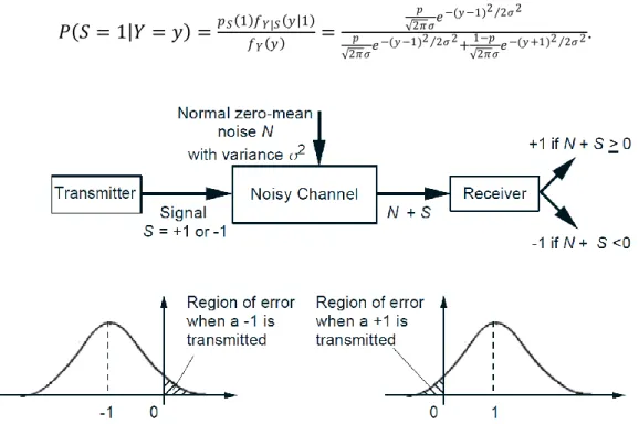
Problem. Let us revisit the signal detection problem. A signal 𝑆 is transmitted and we are given that 𝑃(𝑆 = 1) = 𝑝 and 𝑃(𝑆 = −1) = 1 − 𝑝. The received signal is 𝑌 = 𝑁 + 𝑆, where 𝑁 is
zero mean normal noise, with variance 𝜍2, independent of 𝑆. What is the probability that 𝑆 = 1,
Solution: Conditioned on 𝑆 = 𝑠, the random variable 𝑌 has a normal distribution with
mean 𝑠 and variance 𝜍2. Applying the formula, we obtain
𝑃 𝑆 = 1 𝑌 = 𝑦 =𝑝𝑆 1 𝑓𝑌|𝑆 𝑦 1
𝑓𝑌 𝑦 =
𝑝
2𝜋 𝜍𝑒−(𝑦 −1)2 2𝜍 2 𝑝
2𝜋𝜍𝑒−(𝑦 −1)2 2𝜍 2+ 1−𝑝
2𝜋𝜍𝑒−(𝑦 +1)2 2𝜍 2
.
Figure 1: The signal detection scheme. The area of the shaded region gives the probability of error in the two cases where −1 and +1 is transmitted.
Problem. Let 𝑋 be exponentially distributed with mean 1. Once we observe the experimental value 𝑥 of 𝑋, we generate a normal random variable 𝑌 with zero mean and variance
𝑥 + 1. What is the joint PDF of 𝑋 and 𝑌?
Solution: We have 𝑓𝑋(𝑥) = 𝑒−𝑥, for 𝑥 ≥ 0, and
𝑓𝑌|𝑋(𝑦|𝑥) = 2𝜋(𝑥+1)1 𝑒−𝑦2/2(𝑥+1).
Thus,
𝑓𝑋,𝑌(𝑥, 𝑦) = 𝑓𝑋(𝑥)𝑓𝑌|𝑋(𝑦|𝑥) = 𝑒−𝑥 1 2𝜋(𝑥+1)𝑒
−𝑦2/2(𝑥+1)
,
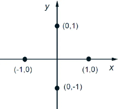
Problem. The pair of random variables (𝑋, 𝑌) takes the values (1, 0), (0, 1), (−1, 0), and
(0, −1), each with probability 1/4 (see Fig. 2). Thus, the marginal PMFs of 𝑋 and 𝑌 are
symmetric around 0, and 𝐸[𝑋] = 𝐸[𝑌] = 0. Furthermore, for all possible value pairs (𝑥, 𝑦),
either 𝑥 or 𝑦 is equal to 0, which implies that 𝑋𝑌 = 0 and 𝐸[𝑋𝑌] = 0. Therefore,
cov 𝑋, 𝑌 = 𝐸 𝑋 − 𝐸 𝑋 𝑌 − 𝐸 𝑌 = 𝐸 𝑋𝑌 = 0,
and 𝑋 and 𝑌 are uncorrelated. However, 𝑋 and 𝑌 are not independent since, for example, a
nonzero value of 𝑋 fixes the value of 𝑌 to zero.
Figure 2: Joint PMF of 𝑋 and 𝑌. Each of the four points shown has probability 1/4. Here 𝑋 and
𝑌 are uncorrelated but not independent.
Problem. Consider 𝑛 independent tosses of a biased coin with probability of a head equal to 𝑝. Let 𝑋 and 𝑌 be the numbers of heads and of tails, respectively, and let us look at the
correlation of 𝑋 and 𝑌. Here, for all possible pairs of values (𝑥, 𝑦), we have 𝑥 + 𝑦 = 𝑛, and we
also have 𝐸[𝑋] + 𝐸[𝑌] = 𝑛. Thus,
𝑥 − 𝐸[𝑋] = − 𝑦 − 𝐸[𝑌] , for all possible (𝑥, 𝑦).
We will calculate the correlation coefficient of 𝑋 and 𝑌, and verify that it is indeed equal to −1.
We have
cov 𝑋, 𝑌 = 𝐸 𝑋 − 𝐸 𝑋 𝑌 − 𝐸 𝑌 = −𝐸 𝑋 − 𝐸 𝑋 2 = −var(𝑋).
𝜌 = cov (𝑋,𝑌)
var (𝑋)var (𝑌)=
var (𝑋)
var (𝑋)var (𝑋)= −1.
Problem. Consider four random variables, 𝑊, 𝑋, 𝑌, 𝑍, with 𝐸[𝑊] = 𝐸[𝑋] = 𝐸[𝑌] =
𝐸[𝑍] = 0, var(𝑊) = var(𝑋) = var(𝑌) = var(𝑍) = 1, and assume that 𝑊, 𝑋, 𝑌, 𝑍 are pairwise
uncorrelated. Find the correlation coefficients of 𝜌(𝐴, 𝐵) and 𝜌(𝐴, 𝐶), where 𝐴 = 𝑊 + 𝑋,
𝐵 = 𝑋 + 𝑌, and 𝐶 = 𝑌 + 𝑍.
Solution: We have
cov(𝐴, 𝐵) = 𝐸[𝐴𝐵] − 𝐸[𝐴]𝐸[𝐵] = 𝐸[𝑊𝑋 + 𝑊𝑌 + 𝑋2+ 𝑋𝑌] = 𝐸[𝑋2] = 1,
and
var(𝐴) = var(𝐵) = 2,
so
𝜌(𝐴, 𝐵) = cov (𝐴,𝐵)
var (𝐴)var (𝐵)= 1 2.
We also have
cov(𝐴, 𝐶) = 𝐸[𝐴𝐶] − 𝐸[𝐴]𝐸[𝐶] = 𝐸[𝑊𝑌 + 𝑊𝑍 + 𝑋𝑌 + 𝑋𝑍] = 0,
so that
𝜌(𝐴, 𝐶) = 0.
Problem. Joint PMF of two RVs is:
𝑌𝑖 𝑋𝑖
0 2 5
1 0.1 0 0.2
2 0 0.3 0
4 0.1 0.3 0
Find numerical characteristics: 𝐸[𝑋], 𝐸[𝑌], var[𝑋], var[𝑌], cov(𝑋, 𝑌) and 𝜌(𝑋, 𝑌).
Find 𝑃𝑋(𝑥) and 𝑃𝑌 𝑦 :
𝑃𝑋 𝑥 = 1 = 0.1 + 0 + 0.2 = 0.3;
𝑃𝑋 𝑥 = 2 = 0 + 0.3 + 0 = 0.3;
𝑃𝑋 𝑥 = 4 = 0.1 + 0.3 + 0 = 0.4;
𝑃𝑌 𝑦 = 0 = 0.1 + 0 + 0.1 = 0.2;
𝑃𝑌 𝑦 = 2 = 0 + 0.3 + 0.3 = 0.6;
𝑃𝑌 𝑦 = 5 = 0.2 + 0 + 0 = 0.2.
Expectation and variance of 𝑋 and 𝑌:
𝐸 𝑋 = 1 ∙ 0.3 + 2 ∙ 0.3 + 4 ∙ 0.4 = 2.5;
𝐸 𝑋2 = 1 ∙ 0.3 + 4 ∙ 0.3 + 16 ∙ 0.4 = 7.9;
var 𝑋 = 𝐸 𝑋2 − 𝐸 𝑋 2 = 7.9 − 6.25 = 1.65;
𝐸 𝑌 = 0 ∙ 0.2 + 2 ∙ 0.6 + 5 ∙ 0.2 = 2.2;
𝐸 𝑌2 = 0 ∙ 0.2 + 4 ∙ 0.6 + 25 ∙ 0.2 = 7.4;
var 𝑌 = 𝐸 𝑌2 − 𝐸 𝑌 2 = 7.4 − 4.84 = 2.56.
Covariance and correlation:
𝐸 𝑋𝑌 = 𝑥,𝑦𝑥𝑦𝑝𝑋𝑌(𝑥𝑦)= 0 ∙ 1 ∙ 0.1 + 2 ∙ 1 ∙ 0 + 5 ∙ 1 ∙ 0.2 + 0 ∙ 2 ∙ 0 + 2 ∙ 2 ∙ 0.3 + 5 ∙ 2 ∙ 0 + 0 ∙ 4 ∙ 0.1 + 2 ∙ 4 ∙ 0.3 + 5 ∙ 4 ∙ 0 = 1 + 1.2 + 2.4 = 4.6;
cov 𝑋, 𝑌 = 𝐸 𝑋𝑌 − 𝐸 𝑋 𝐸 𝑌 = 4.6 − 2.5 ∙ 2.2 = −0.9;
𝜌 𝑋, 𝑌 = cov 𝑋,𝑌
var 𝑋 var 𝑌 =
−0.9