Dynamics of a double-stranded DNA segment in a shear flow
Debabrata Panja
Institute for Theoretical Physics, Universiteit Utrecht, Leuvenlaan 4, 3584 CE Utrecht, The Netherlands
Gerard T. Barkema
Institute for Theoretical Physics, Universiteit Utrecht, Leuvenlaan 4, 3584 CE Utrecht, The Netherlands and Instituut-Lorentz, Universiteit Leiden, Niels Bohrweg 2, 2333 CA Leiden, The Netherlands
J. M. J. van Leeuwen
Instituut-Lorentz, Universiteit Leiden, Niels Bohrweg 2, 2333 CA Leiden, The Netherlands (Received 24 December 2015; published 7 April 2016)
We study the dynamics of a double-stranded DNA (dsDNA) segment, as a semiflexible polymer, in a shear flow, the strength of which is customarily expressed in terms of the dimensionless Weissenberg number Wi. Polymer chains in shear flows are well known to undergo tumbling motion. When the chain lengths are much smaller than the persistence length, one expects a (semiflexible) chain to tumble as a rigid rod. At low Wi, a polymer segment shorter than the persistence length does indeed tumble as a rigid rod. However, for higher Wi the chain does not tumble as a rigid rod, even if the polymer segment is shorter than the persistence length. In particular, from time to time the polymer segment may assume a buckled form, a phenomenon commonly known as Euler buckling. Using a bead-spring Hamiltonian model for extensible dsDNA fragments, we first analyze Euler buckling in terms of the oriented deterministic state (ODS), which is obtained as the steady-state solution of the dynamical equations by turning off the stochastic (thermal) forces at a fixed orientation of the chain. The ODS exhibits symmetry breaking at a critical Weissenberg number Wic, analogous to a pitchfork bifurcation in dynamical systems. We then follow up the analysis with simulations and demonstrate symmetry breaking in computer experiments, characterized by a unimodal to bimodal transformation of the probability distribution of the second Rouse mode with increasing Wi. Our simulations reveal that shear can cause strong deformation for a chain that is shorter than its persistence length, similar to recent experimental observations.
DOI:10.1103/PhysRevE.93.042501 I. INTRODUCTION
The flow properties of a solution of polymers have attracted the interest of physicists for a long time. One side of the problem concerns how the concentration of dissolved polymers influences, e.g., the viscous (or viscoelastic) prop-erties of the fluid. The other side concerns how fluid flow influences the behavior of polymers. Here we restrict ourselves to the latter. Specifically, we consider a dilute solution of double-stranded DNA (dsDNA) segments in water under shear. Double-stranded DNA is a semiflexible polymer, since it preserves mechanical rigidity over a range, characterized by the persistence lengthlp ≈40 nm [1,2], along its contour.
That a polymer will go through a “coil-stretch transition” under the influence of a shear flow was originally predicted by de Gennes [3], although it would be more than two decades before the coil-stretch transition would be put to experimental verification. Interestingly, however, the first key experiment along this line—combining fluid flow and fluorescence microscopy techniques (the latter in order to visually track polymers)—was performed to determine the force-extension curve of dsDNA, wherein uniform water flow was used to stretch (end-tethered) polymers [4]. Extending that experimental setup to include more complicated flow patterns, such as elongational flow [5,6] and shear flow [7,8] soon followed, driven by the quest to understand how flow-induced conformational changes take place in polymers (see, e.g., Ref. [9] for a review).
An intriguing by-product of the experiments with shear flow was the tumbling motion of the chains, which can be tracked
by, e.g., the relative orientation of the polymer’s end-to-end vector with respect to the direction of the flow [7,8]. Although irregular at short time scales, a tumbling frequency could be defined based on the long-time statistics of the chain’s orientation. The tumbling behavior soon started to receive further attention from researchers: Over the last decade and a half, a number of models have been constructed [10–12] and further experiments have been performed [13–16] to characterize and quantify the tumbling behavior, in particular, the dependence of the tumbling frequency on the shear strength. The subject of this paper, too, is tumbling behavior in a shear flow, specifically for a dsDNA chain that is smaller than its persistence length.
As stated earlier, the shear strength ˙γ is customarily expressed by the dimensionless Weissenberg number Wi=
˙
γ τ, where τ is a characteristic time scale for the polymer. At one extreme, for flexible polymers (polymer segments that are many times longer than their persistence length, assuming coil configurations in the absence of shear), which many of the above studies focus on, the natural choice for
frequency scales as f ∝Wi2/3 [16–18]. (Given that the physics of tumbling is different for flexible and semiflexible polymers, the similarity in the scaling behavior of f is striking.)
Recently, Harasimet al.[16] experimented with tumbling f-actin segments of several lengths (∼3–40μm) in a shear flow. They found that the tumbling frequencyffollows the lawf ∝
Wi2/3 for small Weissenberg numbers. A closer inspection of their data reveals significant deviations from thef ∝Wi2/3 power law around and above the persistence length (≈16μm). Images and movies out of the experiments have revealed that f-actin segments of lengths smaller than the persistence length can strikingly buckle intoJ andUshapes, broadly known as Euler buckling.
These issues of buckling and the tumbling frequency were taken up by Lang et al. [12] by an extensive modeling study, using the inextensible wormlike chain as Hamiltonian. They discussed the tumbling frequency for the whole range spanning the two extremes, i.e., from flexible to semiflexible polymer segments, and reported, in the intermediate regime, the dependencef ∝Wi3/4.
The present paper has been inspired by the experiment of Harasimet al. [16]. Our focus is to provide a quantitative characterization of the Euler buckling, and the corresponding shapes of a tumbling semiflexible polymer segment in a shear flow. To this end, we take advantage of a recently developed bead-spring model for semiflexible polymers [19,20] and its highly efficient implementation on a computer [21]. We model dsDNA segments dynamics for lengths20 nm, and analyze their dynamics in terms of the Rouse modes [22]. The persistence length of dsDNA is ≈40 nm, corresponding to
≈120 beads with the average intrabead distance ≈0.33 nm, the length of a dsDNA base pair. We show that the tumbling frequency adheres to the rigid-rod results at low Wi and that for high Wi, semiflexible polymer segments tumble much faster. This difference quickly leads us to issues related to (Euler) buckling of the chain under the influence of shear. We first analyze Euler buckling in terms of the oriented deterministic state (ODS), which results from turning off the stochastic (thermal) forces in polymer dynamics at a fixed orientation of the chain. In this state the internal forces, tending to keep the chain straight, balance the shear forces. Below a critical Weissenberg number Wic, the ODS shows a slightly bentS shape. Above Wica symmetry breaking takes place, analogous to pitchfork bifurcation, where the ODS strongly deviates from a rigid rod.
We follow up the ODS analysis with simulations and demonstrate symmetry breaking in computer experiments, and demonstrate that, similar to the experimental snapshots found for f-actin filaments in Ref. [16], shear can cause strong deformation, even for a chain that is shorter than its persistence length.
The structure of the paper is as follows. In Sec. II we introduce the model. In Sec. III we describe the polymer dynamics in terms of the Rouse modes. In Sec. IV we analyze the time evolution of the orientation of the polymer, from which we determine the tumbling frequency. In Sec.V
we analyze Euler buckling, identify the critical Weissenberg number Wic and solve for the shapes of the polymer in the ODS. We follow up the theory of Sec.Vwith simulations in
Sec.VI, and end the paper with a discussion in Sec.VII. See the Supplemental Material [23] for a movie of a tumbling dsDNA segment—details on the movie are provided in Sec.VI.
II. THE MODEL
The Hamiltonian for our bead-spring model for semiflexible polymers, the details of which can be found in our earlier works [19–21], reads
H= λ
2 N
n=1
(|un| −d)2−κ N−1
n=1
un·un+1, (1)
with stretching and bending parametersλandκ, respectively. Hereunis the bond vector between the (n−1)th and thenth beads
un=rn−rn−1, (2)
andrnis the position of the nth bead (n=0,1, . . . ,N). The parameterd provides a length scale by the use of which we reduce the Hamiltonian to
H
kBT = 1
T∗
N
n=1
(|un| −1)2−2ν N−1
n=1
un·un+1
, (3)
with dimensionlessν=κ/λandT∗=kBT /(λd2) parametriz-ing the Hamiltonian. In this formulation the persistence length of the polymer is given bylp=(ν/T∗)d/(1−2ν). The model is a discrete version of the polymer withNdiscretization units (i.e., of length N). From the analysis of the ground state of the Hamiltonian (3) [19–21], each discretization unit can be shown to have a lengtha=d/(1−2ν).
The parameters of the model—T∗ andν—are determined by matching to the force-extension curve. For dsDNA, our semiflexible polymer of choice in this paper, we use a=
0.33 nm, the length of a dsDNA base pair, which leads toT∗=0.034 andν=0.353, meaning that one persistence length corresponds toN≈120 [19–21].
III. POLYMER DYNAMICS A. Construction of the Rouse modes modes
We analyze the dynamics of the polymer by its Rouse modes, since they turn out to be a convenient scheme for solving the equations of motion with a sizable time step, without introducing large errors [21].
The representation of the configurations of a polymer chain in terms of its fluctuation modes uses basis functions. The well-known Rouse modes employ the basis functions
φn,p=
2
N+1
1/2 cos
(n+1/2)pπ N+1
, (4)
such that conversion of positionsrnto Rouse modesRp and vice versa are given by
Rp=
n
rnφn,p, rn=
p
φn,pRp. (5)
center-of-mass motion by always measuring the bead positions with respect to the center of mass.
B. The equations for the Rouse modes under shear We consider the situation where water flows in the ˆx direction, with a shear gradient ˙γ in the ˆy direction. The Langevin equation for the motion of the bead positionrnthen reads
drn
dt = −
1
ξ ∂H ∂rn
+γ˙(yn−Yc.m.)ˆx+kn. (6)
The HamiltonianHis given in Eq. (1), andξ is the friction coefficient due to the viscous drag, acting on each bead. The first term on the right hand side of the equation represents the internal force, which tends to keep the chain straight. The second term is the shear force due to the flow, where ˙γ is the shear rate,Yc.m.is they coordinate of the center of mass of the chain, and yn is the y coordinate of monomern. As mentioned earlier, we measure the bead positions with respect to the location of the chain’s center of mass, leading to the term
∝(yn−Yc.m.). The last term in Eq. (6) gives the influence of the random thermal forcekn, which has the correlation function
knα(t)kmβ(t)=(2kBT /ξ)δα,βδn,mδ(t−t). (7)
In order to work with dimensionless units we replace the timetwith
τ =λt /ξ. (8)
The ratioξ /λthen becomes the microscopic time scale, such that τ is dimensionless. In the same spirit we combine the shear ratio ˙γwith this time scale, leading to the dimensionless constantgas the shear strength
g=γ˙ξ
λ. (9)
The shear strength is customarily expressed in terms of the Weissenberg number, which we define as
Wi= γ˙ 2Dr
with Dr =
kBT
I ξ . (10)
Here Dr is the rotational diffusion constant with I as the moment of inertia of the polymer segment in its ground state (of the Hamiltonian). The relation between the two dimensionless quantities Wi andgis then given by
Wi=g I0
2T∗, (11)
whereI0 =I /d2, the dimensionless moment of inertia of the polymer segment in the ground state.
Using the orthogonal transformation converting positions into modes the dynamic equations for the Rouse modes can be cast in the form [21]
dRp
dτ = −ζpRp+Fp+Hp+Kp. (12)
For the decay constant we use the expression
ζp =4ν
1−cos
pπ N+1
2
. (13)
This spectrum follows from a subtraction in the coupling forceHp, which derives from the contour length term in the Hamiltonian [21]
Hp =
2
N+1
1/2
n sin
pnπ N+1
un
1
un
−1+2ν
.
(14) The subtraction 1−2ν within the last parentheses changes the Rouse spectrum from longitudinal to the transverse form Eq. (13). Finally,Fpis the shear force given by
Fp =gxˆ(ˆy·Rp). (15)
The fluctuating thermal forceKα
p is the orthogonal transform of theknin Eq. (7),
Kpα(τ)Kqβ(τ)=2T∗δα,βδp,qδ(τ−τ). (16)
Although the Rouse modes turn out to be a convenient scheme for solving the equations of motion with a sizable time step without large errors, we do pay a computational penalty in the calculation of the coupling force, which requires a transformation (8) from the Rouse modes to the bond vectors and the transformation (14) back to the modes. The penalty can be kept to the minimum by the use the fast Fourier transform (FFT) to switch from modes to bead positions; it keeps the number of operations of the orderNlogN.
C. Body-fixed coordinate system to analyze tumbling dynamics One of the major quantities of interest in the tumbling process is the dynamics of the orientation of the polymer. The orientation can be defined in several ways. The most common one is the direction of the end-to-end vector. Since the ends of the chain fluctuate substantially over short-time scales, this is not a slow variable. We prefer to use as orientation the direction of the first Rouse mode R1, which is the slowest decaying mode. We therefore define the orientation ˆnof the polymer as
ˆ
n=R1ˆ . (17)
We refer to the components of the Rouse modes in the direction of ˆnas longitudinal components
Rlp=nˆ·Rp. (18)
The perpendicular directions are transverse to ˆn. The first Rouse mode has, by definition, only a longitudinal component. In practice, the so-defined orientation does not differ much from the direction of the end-to-end vector.
Further, it is convenient to discuss the temporal behavior of the polymer not only in the laboratory-frame coordinate system, with coordinate axes (ˆx,yˆ,z), but also in the body-fixedˆ coordinate system which we define as follows. Along with the unit vector ˆn, one of the two transverse axes, ˆn, is taken perpendicular to ˆnand ˆx, namely,
ˆ
m=nˆ×xˆ/r, r=n2y+n2z1/2. (19)
The mode component in this direction, being perpendicular to ˆ
x, is not influenced by the shear force. The other transverse direction is then naturally obtained as
ˆ
Vector components along ˆsare maximally sheared. The system ( ˆn,ˆs,m) forms an orthogonal basis set. For later use, below weˆ list the Cartesian components of the vectors ( ˆn,ˆs,m):ˆ
nx =sinθcosφ, sx =r, mx=0,
ny =sinθsinφ, sy= −nxny/r, my =nz/r, (21)
nz=cosθ, sz= −nxnz/r, mz= −ny/r.
We denote the components of the modes generically with the indexα, which alternatively runs throughα=(x,y,z) orα=
(n,s,m).
IV. TIME EVOLUTION OF THE ORIENTATION OF THE POLYMER
The evolution of the orientation is given by the dynamics of the two transverse components ofR1,
dnˆ
dτ = d dτ
R1
Rl 1
= dR1
dτ
1
Rl 1
+R1 d
dτ
1
R1 1
= 1
Rl 1
dR1
dτ , (22)
wherein the third equality follows from the fact that the trans-verse components ofR1vanish by definition. So the temporal derivative of the longitudinal component is multiplied the vanishing transverse component. We then use Eq. (12) and get
dnˆ
dτ =gxˆ(ˆy·n)ˆ +(H1+K1)/R
l
1. (23)
Obviously, in the right hand side of the equations only the transverse components of the vectors are relevant.
For the interpretation of Eq. (23) we note thatR1l is closely related to the moment of inertiaIof the chain, which is defined as
I d2 =
n
rnl2=
p
Rlp2=
p
Ip, (24)
where Ip is the contribution of thepth Rouse mode to the moment of inertia. When the chain is (relatively) straight, the sum over the modes is heavily dominated by the first componentI1. So it is an indicative approximation to replace
IbyI1.
In the (relatively) straight state the configuration of the chain resembles that of a straight rod. In order to make a connection with the equation of tumbling for a rigid rod, we rewrite the equation using a different scaling of the timeτ. We define the variable ˜τ, linked to the Weissenberg number, as
˜
τ =gτ/Wi, with g/Wi=2T∗/I1, (25)
where we have usedI1as measure for the moment of inertia. In terms of ˜τ, Eq. (23) then becomes
dnˆ
dτ˜ =Wi[ˆx(ˆy·n)]ˆ +( ˜H1+K˜1), (26) with ˜H1and ˜G1defined as
˜ H1=
√
I1
2T∗H1, K˜1( ˜τ)=
√
I1
2T∗K1(τ). (27)
The new random force has a correlation function ˜
K1α( ˜τ) ˜K1β( ˜τ)=δα,βδ( ˜τ−τ˜). (28)
10
-110
010
110
210
310
410
510
6Wi
10
-210
010
210
410
6f
rigid rod formula
N
= 7
N
= 15
N
= 31
N
= 63
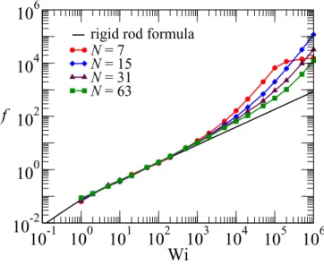
FIG. 1. The tumbling frequency as a function of the Weissenberg number Wi for a series of chain lengths N=7, 15, 31, and 63. The conversion to Weissenberg numbers is based on the ground-state moment of inertia [see Eq. (11)].
Apart from the mode-coupling term ˜H1, Eq. (26) is the same as that of an infinitely thin rigid rod [18]. Therefore, it makes sense to compare the tumbling frequencyf with that of the rigid rod, given by [18]
f = Wi
4π(1+0.65 Wi2)1/6. (29) For comparison we show in Fig.1the tumbling frequency of dsDNA chains for several lengths shorter than the persistence length (which corresponds to N ≈120), as found from simulations, together with that of a rigid-rod expression, Eq. (29). The simulations have been performed using an efficient implementation of semiflexible polymer dynamics [21] of the bead-spring model [19,20]. At any given value of the Weissenberg number, obtained by using the rotational inertia of a rigid rod that has the same configuration as the ground state of the Hamiltonian (3), snapshots of the polymer have been used to calculate its orientation [θ(t),φ(t)] in the laboratory frame. The φ(t) data are then fitted by a straight line to obtain the tumbling frequency.
We point out that the simulations follow the rigid-rod formula for a surprisingly large range of Weissenberg numbers, clearly indicating that up to Wi=100 the mode-coupling force ˜H1 is unimportant. In order to see what this implies for the shear rate ˙γ, using the expressionI /d2=N3/12 for the moment of inertia, we write the relation between Wi and the shear rate ˙γas
Wi=γ˙ a 2ξ
kBT
N3
24. (30)
Note that in Eq. (30) the molecular time scale equals [21]
a2ξ
kBT
=52×10−12s. (31)
of the order of the persistence length, say, N =100, that only the range Wi<2 is presently achievable in the laboratory; i.e., the differences from the rigid-rod behavior in Fig.1lie outside the reach of present day experiments. Nevertheless, the origin of the deviations from the rigid-rod behavior is the-oretically interesting; we will address this issue in the Sec.VI.
V. SHAPES OF SEMIFLEXIBLE POLYMER IN THE ORIENTED DETERMINISTIC STATE
In order to further analyze the tumbling process, it is useful to note that the orientation changes at a slower rate than all the other modes. This prompts us to focus on the configuration which is obtained as the steady-state solution of the dynamical equations by turning off the stochastic (thermal) forces at a fixed orientation of the chain. We call this configuration the oriented deterministic state (ODS). We use the properties of the ODS as indicative for the configurations of the chain at the given orientation.
A. The approach to the oriented deterministic state (ODS) The ODS configuration of the chain is obtained from Eq. (12) by the decay of the equation
dRp
dτ = −ζpRp+Fp+Hp. (32)
The constraint of a fixed orientation is imposed by leaving out the transverse components of the modeR1 and setting them equal to zero in the other mode equations. Asymptotically the configuration obeying Eq. (32) will turn into the ODS. So for the ODS the left hand side of Eq. (32) vanishes. The approach to the ODS configuration as following from Eq. (32) is slow.
A further simplification of finding the asymptotic state of Eq. (32) follows by considering the ODS in the body-fixed system. As there are no shear forces in the ˆm direction, the ODS shape has no component in that direction. For the two other equations in the ( ˆn,ˆs) plane we get in detail
(ζp−gnxny)Rpn−gnxsyRps =H n p,
(33)
gsxnyRpn+(ζp−gsxsy)Rps =H s p.
Forp=1 we have only the first equation since the second refers to the transverse componentR1s, which we keep equal to zero. Solving this set of nonlinear equations is delicate. We found that, under normal circumstances, iteration is a stable and quick way to the solution. For a given orientation of the chain, we start with an arbitrary configuration (in fact, for the starting configuration, we use the ground-state config-uration of the chain [19,20]). We then compute the coupling forces Hn
p andHps, solve the two-by-two equations (33) for
Rn p and R
s
p, and construct a new set of bond vectors. We repeat the calculation ofHpnandHpsfor the new configuration and continue the process until the iterative process converges. Iteration leads faster to the ODS than the evolution of the equations, Eq. (32). The results of the two approaches, in any case, coincide.
B. Symmetry breaking in the oriented deterministic state The iterative solution of Eq. (33), as well as the decay towards the ODS on the basis of Eq. (32), reveals an interesting
phenomenon. To show this, we note that configurations that are invariant under reversal of the chain have vanishing even Rouse modes. It is easy to see that Eqs. (33) preserve this symmetry under iteration. The bond vectorsunchange sign under the operation
n↔N−n. (34)
Changing the summation variable from n to N−n in the definition Eq. (14) of the coupling force shows thatHpchanges sign for evenp, but not for oddp. This means that if we start the iteration with a configuration that is invariant under reversal, i.e., we start the iteration with only oddHp on the right hand side of Eq. (33), it leads to a solution that has, once again, only odd Rouse mode components.
The above does not, however, exclude that there are solutions which break the reversal symmetry. The best way to solve for the ODS is to therefore start the iteration with a configuration with a (perturbatively) small even mode, e.g., R2. The perturbation may grow or decrease under successive iterations. We find that for low Weissenberg numbers the perturbation decays to zero, while beyond a critical Weis-senberg number Wic, the reversal symmetry is broken, i.e., the perturbation grows and saturates at a nonzero value, much as the classic case of a pitchfork bifurcation.
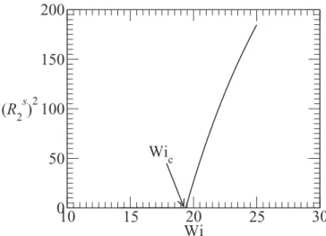
As an example, for a dsDNA chain of length N =63 (note: a dsDNA segment of one persistence length corresponds to N ≈120), we plot the squared value of the transverse component Rs2 as a function of the Weissenberg number in Fig.2. At Wi=Wicthe first nonzero even Rouse modes in the chain appear forθ=π/2 andφ=3π/4. The coefficient ofRs
2in Eq. (33),
ζp−gsxsy =ζp+g(sinθ)2sinφcosφ, (35)
reaches its smallest value for θ=π/2 andφ=3π/4, thus leading to the largest value of R2s in the case of symmetry breaking.
10
15
20
25
30
Wi
0
50
100
150
200
(R
2 s
)
2Wi
cFIG. 2. The squared value of the transverse componentRs 2as a function of the Weissenberg number for a dsDNA chain of length
0.0
0.2
0.4
0.6
0.8
1.0
φ
/
π
160
170
180
190
200
210
end-to-end distance
Wi = 15
(b)
Wi = 20
Wi = 25
0.65
0.70
0.75
0.80
0.85
φ
/
π
0.0
2.0
4.0
6.0
8.0
|
R
2(a)
s|
|
R
4s|
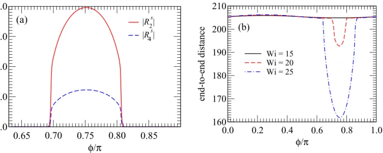
FIG. 3. (a) The appearance of the first two even Rouse modes in a window around the optimal valueφ=3π/4 forθ=π/2 at Wi=21.3. (b) The end-to-end distance as a function ofφforθ=π/2 for some values of Wi around Wic≈19.4.
From Fig.2 we see that the critical Weissenberg number forθ=π/2 andφ=3π/4 equals Wic≈19.4 for a dsDNA chain of lengthN =63.
C. Shapes of the chain and Euler buckling
The shape of the chain depends on its orientation of the polymer, which comes into the solution through the components of the axes ˆnand ˆs. The shear is most effective in thex-y plane, i.e., forθ=π/2. In Fig.3(a), forN =63, we show the value of |R2s| and |Rs4| as a function of φ in the neighborhood of the most effective valueφ=3π/4 for Wi=21.3 and θ =π/2 (note: Wic≈19.4). The nonzero value of|Rs
p|disappears at φ=3π/4 when Wi approaches Wicfrom above.
Further, in order to see the magnitude of the effect, we plot in Fig.3(b)the behavior of the end-to-end distance of the chain forN =63 as a function ofφforθ=π/2 and for some values of Wi around the critical Weissenberg number Wic. One observes that the end-to-end distance varies only slightly as a function of orientation below Wic. Above the Wica large dip develops aroundφ=3π/4, demonstrating that the symmetry breaking goes hand in hand with the so-called Euler buckling of the chain, i.e., the chain folds, which reduces its end-to-end distance.
In order to visually appeal the reader to Euler buckling, we provide a number of snapshots of the chain in the ODS for
N =63 and Wi=100, confined to the x-y plane in Fig.4. This large Weissenberg number is well above Wic. The region ofφwithinπ/2< φ πis the interesting region, for which we plot the polymer configurations.
To conclude, the ODS configuration of the chain resembles a rigid rod below a critical value Wic of the Weissenberg number. Above this critical value,even though the length of the chain is only about half as that of the persistence length, it breaks the reversal symmetry, much as the classic case of a pitchfork bifurcation. This leads to the development of a region aroundθ=π/2 andφ=3π/4, where the chain (Euler)
buckles. The buckling gives a large dip in the end-to-end distance.
Finally, we note that the critical Wicdepends on the length
N of the chain (roughly inversely proportional) and on ν
(decreasing withν). Converting it to a critical shear rate ˙γc involves alsoT∗[see Eq. (25)].
VI. SHAPES OF A TUMBLING SEMIFLEXIBLE POLYMER: SIMULATIONS
Our simulations have been performed using an efficient implementation of the semiflexible polymer dynamics [21] of the bead-spring model [19,20].
-80
-60
-40
-20
0
20
40
60
x
-60
-40
-20
0
20
40
y
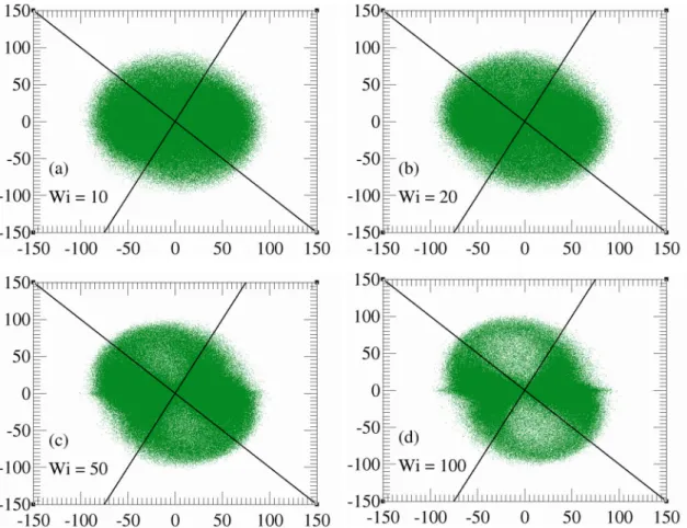
FIG. 5. Scatter plots ofRs
2as a function ofφaroundθ=π/2 at four values of Wi of lengthN=63. In between the solid lines, representing 0.35π < φ <3π/4, we see the probability distributionP(Rs
2) ofRs2changing with increasing Wi. We take these issues up in Fig.6. See also the text for details.
Before we discuss the details of the simulation results, we make the readers aware of the differences between the ODS in Sec.Vand the simulations. Thermal noise plays no role in the ODS, while in simulations it does. This implies that although for Wi<Wic the amplitude ofRs2 is identically zero in the ODS, we should not expect to find the same in simulations at low Wi values, since in simulations the second Rouse mode will always be kicked up by noise. This calls into question the relevance of the ODS for simulations—in particular, whether the tumbling of the chain is sufficiently slow such that the simulation can explore the neighborhood of the ODS, and thereby follow the characteristics of the ODS. In view of the lack of clarity for an answer to this question, we used the ODS as a guide for the simulations: To be more precise, we focused on the values of Wi in the range 10Wi100 forN =63 and sampled the probability distribution ofRs2as a function of the orientation.
In simulations for dsDNA of lengthN =63 we recorded 16 million consecutive snapshots of the chain at regular intervals, R1 (for determining the orientation of the chain) andR2, at equal intervals of time, for several values of Wi. The angles (θ,φ) for the chain’s orientation are determined from the values of R1. We then selected out the snapshots in this slice|θ−π/2| =0.1 rad, leaving us with 2–3 million snapshots dependent on the value of Wi. In Fig.5 we show the corresponding scatter plots ofRs2 as a function ofφ in this slice at four values of Wi. In between the solid lines,
representing 0.35π < φ <3π/4, we see two lobes of empty regions developing, signaling that the probability distribution
P(Rs 2) ofR
s
2for these values ofφchanges with increasing Wi. We note that the values of φcorresponding to the two solid lines in Fig.5are chosen solely by visual inspection, and that the locations of the empty lobes are shifted with respect to the region inφ, for which the ODS exhibits Euler buckling.
In order to further study the change in the probability distribution P(R2s) of R2s, we selected out the data points corresponding to 0.35π < φ <3π/4 in Fig. 5, leaving us 50 000–100 000 data points. From them we constructed the probability distributionP(Rs
2). The distributions, correspond-ing to Wi=10, 15, 20, 25, 50, and 100, are shown in Fig.6. In Fig.6(a)we see that the unimodal distribution for Wi=10 gradually transforms into a bimodal distribution symmetric aroundRs2=0 for higher Wi. This development is the telltale sign of symmetry breaking, which can also be tracked by the development of the Binder cumulantB, defined as
B=1− R
s 2
4
3 R2s2
, (36)
-120 -80 -40 0 40 80 120
R
s20.00 0.03 0.06 0.09 0.12
P
(
R
s
)
2Wi = 10 Wi = 15 Wi = 20 Wi = 25 Wi = 50 Wi = 100
(a)
0
20
40
60
80
100
120
Wi
0.20
0.30
0.40
0.50
0.60
0.70
B
(b)
FIG. 6. (a) Probability distribution P(Rs 2) of R
s
2 corresponding to 0.35π < φ <3π/4 in Fig. 5 forN=63, showing the unimodal distribution for Wi=10 gradually transforming into a bimodal distribution symmetric aroundRs
2=0 for higher Wi. (b) The corresponding Binder cumulantB, as defined in Eq. (36), which changes from≈0.3 at Wi=10 to≈0.53 at Wi=100.
δpeaks. For the data in Fig.6(a)we see that the value ofB
changes from≈0.3 at Wi=10 to≈0.53 at Wi=100. The symmetry breaking is certainly not confined toN =63. The same analysis on the simulation data (again, all data points within|θ−π/2| =0.1 and 0.35π < φ <3π/4, with the corresponding figures, analogous to Fig. 6, presented in Fig. 7) reveals symmetry breaking taking place also for
N =31.
We note that the center of the region where the symmetry breaking takes place is around the values ofφ≈0.55π, as can be observed from the scatter plots. This is substantially different from the value φ=0.75π, where the onset of buckling takes place in the ODS. The chain tumbles in the direction fromφ=π towardsφ=0. So the buckling in the simulation lags behind with respect to the ODS. This is likely the result of the slowness by which the buckled state is formed
and is broken down. Using Eq. (32) we estimated the time
τ, which is needed to evolve from the ground state (in which the transverse R2
2 =0) to 50% of its asymptotic value (the ODS), to be of the order τ 106. This translates into a timeτ˜≈0.3 [see Eq. (25)]. In order to put this estimate in perspective, we compare it with the tumbling period 1/f of the rigid rod, which is 1.7 for Wi=20 according to Eq. (29). In other words, the chain indeed travels a sizable fraction of the period in the building-up phase of the buckling, the more so since it rotates faster for the buckling orientations than in the position aligned with the flow.
Thus, to summarize this section, using the theoretical analysis of symmetry breaking as a guide, we have computed the probability distribution P(Rs
2) of R s
2 by simulations of a tumbling dsDNA segment of length N =63 andN =31. The simulation data have confirmed that symmetry breaking
-45
-30
-15
0
15
30
45
R
s20.00
0.05
0.10
0.15
0.20
P
(
R
s
)
2Wi = 10 Wi = 15 Wi = 20 Wi = 25 Wi = 50 Wi = 100
(a)
0
50
100
150
200
Wi
0.20
0.30
0.40
0.50
0.60
0.70
B
(b)
FIG. 7. (a) Probability distribution P(Rs 2) of R
s
2 corresponding to 0.35π < φ <3π/4 in Fig. 5 forN=31, showing the unimodal distribution for Wi=10 slowly transforming into a bimodal distribution symmetric aroundRs
-100
-50
0
50
100
x
-10
-5
0
5
10
y
(b)
-30 -20 -10
0
10
20
30
40
50
x
-40
-20
0
20
40
60
y
(a)
FIG. 8. Simulation snapshots of a tumbling dsDNA chain of lengthN=63 at Wi=100, projected on thex-yplane: (a)Ushape, (b)S
shape.
takes place, showing up as the transition from an unimodal probability distributionP(R2s) ofRs2at Wi=10, transforming into a bimodal distribution symmetric aroundRs2=0, as well as the associated Binder cumulants.
To supplement the above analysis of the simulation data, we show in Fig.8 two simulation snapshots of a tumbling dsDNA chain of lengthN =63 at Wi=100, projected on the
x-yplane, in order to showcase that, akin to the experimental snapshots shown for f-actin in Ref. [16], shear can cause strong deformation even for a chain that is shorter than its persistence length. See the Supplemental Material for a movie of this tumbling chain (that includes both configurations of Fig.8). In the movie, the center of mass of the chain always remains at the origin of the coordinate system. The movie contains 3000 snapshots, with consecutive snapshots being
τ =560 apart in time. Withτ =1 representing 0.16 ps [21], the full duration of the movie spans ≈2.7μs in real time.
VII. CONCLUSION
Our study focuses on fragments of dsDNA, which are fairly extensible semiflexible polymers. The extensibility of dsDNA implies parameters in our Hamiltonian, which admit mode dynamics with a large time step. The usual workhorse for theoretical studies is the inextensible wormlike chain model for the Hamiltonian, the computer implementation of which is confined to significantly smaller time steps.
Our simulations of a semiflexible polymer (dsDNA frag-ments smaller than the persistence length) show that their tumbling frequency is given, for the accessible range of Weissenberg numbers (Wi<2), by the thin rigid-rod formula. Deviations of the tumbling frequency from this formula (Fig.1) occur at higher Weissenberg numbers. It is theoreti-cally interesting to speculate about the nature of the deviations from the rigid-rod formula, also in view of the observation that the accessible range of Weissenberg numbers is much larger for stiffer and longer polymers, e.g., f-actin. The Weissenberg number for a polymer chain is a product of the shear rate ˙γand
the rotational diffusion time scale of a rigid rod of the same length as the chain, i.e., L. Consequently, the Weissenberg number∝γ L˙ 3. One persistence length of f-actin is about 200 times longer than one persistence length of dsDNA. In units of persistence length, for the same shear rate, one thus reaches orders of magnitude higher Weissenberg numbers for f-actin than for dsDNA.
In this respect we note that the Wi2/3law for rigid thin rods originates from a singularity that develops in the probability distribution for the orientation in the pointsθ =π/2 andφ=0 or π [18]. The reason is that a thin rigid rod does not feel a torque from the shear in the aligned orientation and only a fluctuation can pull the rod over this stagnation point. A semiflexible polymer, however, always feels a torque due to fluctuations of the other modes (either thermal or buckling), which communicate with the orientation through the coupling forceH1. These fluctuations enable Jeffery-like orbits which are characteristic for ellipsoids with a finite aspect ratio in the moments of inertia [24]. The deviations from the thin rigid-rod formula that we see in Fig.1do not substantiate thef ∝Wi3/4 law reported for inextensible wormlike chains [12].
Using our Hamiltonian we have made a quantitative analysis of the phenomenon of Euler buckling. Fixing the orientation and searching for the configuration which results by turning off the thermal noise yields the oriented deterministic state (ODS). In the ODS we see a sharply defined critical Wic above which the buckling occurs. It is a form of symmetry breaking through the occurrence of even modes in the ODS above Wic.
In the simulations we observe correspondingly a transition in the probability distribution for the even modes, in particular,
Rs
[1] C. Bustamante, J. F. Marko, E. D. Siggia, and S. Smith,Science 265,1599(1994); J. F. Marko and E. D. Siggia,Macromolecules 28,8759(1995).
[2] M. D. Wang, H. Yin, R. Landick, J. Gelles, and S. M. Block, Biophys. J.72,1335(1997).
[3] P. G. de Gennes,J. Chem. Phys.60,5030(1974).
[4] T. T. Perkins, D. E. Smith, R. G. Larson, and S. Chu,Science 268,83(1995).
[5] T. T. Perkins, D. E. Smith, and S. Chu,Science276,2016(1997). [6] D. E. Smith and S. Chu,Science281,1335(1998).
[7] D. E. Smith, H. P. Babcock, and S. Chu,Science 283,1724 (1999).
[8] P. LeDuc, C. Haber, G. Bao, and D. Wirtz, Nature (London) 399,564(1999).
[9] E. Shaqfeh, J. Non-Newtonian Fluid Mech. 130, 1 (2005).
[10] M. Chertkov, I. Kolokolov, V. Lebedev, and K. Turitsyn,J. Fluid Mech.531,251(2005).
[11] A. Celani, A. Puliafito, and K. Turitsyn,Europhys. Lett.70,464 (2005).
[12] P. S. Lang, B. Obermayer, and E. Frey,Phys. Rev. E89,022606 (2014).
[13] P. S. Doyle, B. Ladoux, and J.-L. Viovy,Phys. Rev. Lett.84, 4769(2000).
[14] R. E. Teixeira, H. P. Babcock, E. S. Shaqfeh, and S. Chu, Macromolecules38,581(2005).
[15] C. M. Schroeder, R. E. Teixeira, E. S. G. Shaqfeh, and S. Chu, Phys. Rev. Lett.95,018301(2005).
[16] M. Harasim, B. Wunderlich, O. Peleg, M. Kr¨oger, and A. R. Bausch,Phys. Rev. Lett.110,108302(2013).
[17] G. Jeffery,Proc. R. Soc. London, Ser. A102,161(1922). [18] J. M. J. van Leeuwen and H. W. J. Bl¨ote,J. Stat. Mech.(2014)
P09007.
[19] G. T. Barkema and J. M. J. van Leeuwen,J. Stat. Mech.(2012) P12019.
[20] G. T. Barkema, D. Panja, and J. M. J. van Leeuwen, J. Stat. Mech.(2014)P11008.
[21] D. Panja, G. T. Barkema, and J. M. J. van Leeuwen,Phys. Rev. E92,032603(2015).
[22] P. E. Rouse,J. Chem. Phys.21,1272(1953).
[23] See Supplemental Material athttp://link.aps.org/supplemental/ 10.1103/PhysRevE.93.042501for a movie of a tumbling dsDNA chain (that includes both configurations of Fig.8).