The handle http://hdl.handle.net/1887/20110 holds various files of this Leiden University
dissertation.
Author: Wang, Feijia
a study via coupling and large deviations
Proefschrift
ter verkrijging van
de graad van Doctor aan de Universiteit Leiden,
op gezag van Rector Magnificus prof. mr. P.F. van der Heijden,
volgens besluit van het College voor Promoties
te verdedigen op woensdag 7 november 2012
klokke 10:00 uur
door
Feijia Wang
Beoordelingscommissie: Prof. dr. A.C.D. van Enter Prof. dr. C. K¨ulske
I would like to thank people who have been instrumental in helping this
PhD-project come to a good end.
I would like to thank Prof. Frank Redig and Prof. Frank den Hollander for
accepting me as a PhD student in Leiden. I would like to thank Prof. Redig
for his teachings, his questions, his answers, his guidance, etc: I owe him a
lot. I would like to thank Prof. den Hollander for letting me be part of the
probability theory group and for his additional guidance. I would also like to
thank Dr. Alex Opoku for answering many technical questions and for helping
me to improve the introduction to my thesis. His course on Gibbs measures
was very impressive. I would further like to thank the members of the reading
committee for their critical remarks. Finally, I would like to thank my colleagues
in the probability theory group of the institute for their friendliness and the
1 Introduction 1
1.1 Overview of thesis . . . 4
1.1.1 Conservation of Gibbsianness for lattice spin systems . . . 4
1.1.2 Dynamical Gibbs-non-Gibbs transitions for mean-field spin systems 5 1.1.3 Large deviations for the trajectory of the empirical distribution and empirical measure . . . 8
1.2 Generalities on Gibbs and non-Gibbs measures . . . 8
1.2.1 Gibbs measures . . . 8
1.2.2 Transformation of Gibbs measures and phenomenon of non-Gibbsianness 12 1.2.3 The two-layer picture . . . 13
1.3 Large deviation theory and optimal solutions for rate function . . . 15
1.3.1 Large deviation principle . . . 15
1.3.2 Large deviations for stochastic processes . . . 18
1.3.3 The Feng-Kurtz scheme . . . 19
1.3.4 Uniqueness and non-uniqueness of optimal trajectories . . . 20
2 Transformations of one-dimensional Gibbs measures with infinite-range interaction 27 2.1 Introduction . . . 27
2.2 Gibbs measures and their transformations . . . 28
2.2.1 One-dimensional Gibbs measures . . . 28
2.2.2 Transformations of Gibbs measures . . . 30
2.3 Stochastic single-site transformations . . . 31
2.3.1 The transformed potential . . . 36
2.4.1 Exponentially decaying potential . . . 39
2.4.2 Power-law decaying potential . . . 41
2.5 Finite-block transformations . . . 42
3 Gibbs-non-Gibbs transitions via large deviations: computable examples 45 3.1 Introduction . . . 45
3.2 The Feng-Kurtz scheme, Euler-Lagrange trajectories, bad configurations . . 46
3.3 Diffusion processes with small variance conditioned on the future . . . 48
3.3.1 Brownian motion . . . 49
3.3.2 Brownian motion with constant drift . . . 52
3.3.3 Other rate functions for the initial measure and corresponding behav-ior of Brownian motion . . . 52
3.4 The Ornstein-Uhlenbeck process . . . 56
3.4.1 The Ornstein-Uhlenbeck process with constant external field . . . . 57
3.4.2 General drift. . . 58
3.5 Approximately deterministic walks in d= 1 . . . 60
3.5.1 Constant birth and death rates . . . 62
3.5.2 Mean-field independent spin flips . . . 62
3.5.3 Independent spin-flips in a field . . . 64
4 Large deviations for the trajectory of the empirical distribution and em-pirical measure 69 4.1 Introduction . . . 69
4.2 The trajectory of the empirical distribution: general case . . . 71
4.3 Finite-state space continuous-time Markov chains . . . 73
4.3.1 Hamiltonian trajectories for finite Markov chains . . . 75
4.3.1.1 Two-state symmetric flipping . . . 77
4.4 Diffusion processes . . . 78
4.5 Trajectory of the empirical measure . . . 81
4.5.1 Context and notation . . . 81
4.5.2 Translation invariant sequence of local generators . . . 82
4.5.3 Trajectory of the empirical measure . . . 83
4.5.5 Interacting particle systems . . . 86
Introduction
Statistical mechanics studies the collective statistical properties of a system composed of a
large number of components. The components could, for instance, be particles (in lattice
gas systems, see e.g. Chapters 1–2 of [1] and references therein), (magnetic) spins (in spin
systems for ferromagnets, e.g. theIsing model[32]), pixels (in image analysis [23]), economic
agents (in economics [20]), etc. This thesis focuses on the spin interpretation of the
compo-nents. The spins are usually labeled by vertex sets of some underlying (finite/infinite) graph,
whose connectivity structure determines the interdependence among the spins. Among the
graphs that have been considered in the literature are thed-dimensional integer lattice and
the complete graph. The system on the lattice is called lattice-spin system. Here the
un-derlying geometry of the lattice plays a crucial role. The case on the complete graph is
referred to as a mean-field spin system. Here there is no geometry.
In equilibrium statistical mechanics, such a study begins by prescribing aHamiltonian1
Hthat associates to each microscopic description (configuration)σ of the system an energy.
Usually H comes with several parameters such as temperature, external field, chemical
potential etc. depending on the system under consideration. Given an H, the equilibrium
behavior of the system is modeled by the Gibbs probability measureµon the configurations
that takes the form, in finite volume,
µ(σ)∝e−H(σ). (1.0.1) In the thermodynamic limit, e.g., on the full lattice Zd, formula (1.0.1) does no longer
make sense. To give meaning to H, one measures the energy HΛζ of the system in a finite
window Λ of the lattice when everything outside the window is fixed to a configuration ζ.
Thus for any pair of Λ andζ, the associatedfinite-volume Gibbs measure
µζΛ(σ)∝e−HΛζ(σ) (1.0.2) 1
Figure 1.1: Diagram of renormalization group transformation
(the Boltzmann-Gibbs distribution) describes the equilibrium behavior of the system in Λ
when everything outside Λ is set toζ. The family γ of all finite-volume Gibbs measures µζΛ
is said to be a Gibbs specification if µζΛ is “continuous (quasilocal)”as a function of ζ. A
probability measureµ on the configurations is aGibbs measureassociated with H if it has
γ as a version of its conditional distributions. The relations (1.0.2) are referred to as the
DLR equations, after Dobrushin [8, 9], Lanford and Ruelle [37] who introduced them in the
1960s. There can be one or more Gibbs measures associated with the Gibbs specification
γ. The non-uniqueness of Gibbs measures indicates the occurrence of a first-order phase
transition, such a transition accompanied with the presence of spontaneous magnetization,
and uniqueness is an indication of the lack of a first-order phase transition. For more
background on Gibbs measures, we refer the reader to [13, 19, 24, 39]. In what follows
we say that a spin system is Gibbsian if it has a Gibbs measure describing its equilibrium
behavior.
The main question that laid the basis of an area of research is whether a transformed
Gibbsian spin system will remain Gibbsian. This question originated from the study of
renormalization group transformations, a technique for studying phase transitions and
crit-ical phenomena. A renormalization group transformation R is a map from the space of
Hamiltonians onto itself. For such a map to be useful it has to be well defined. But as
Griffiths and Pearce [27, 28] pointed out in the late 1970’s, there is a serious problem when
it comes to precisely defining the mapR. The mapRon HamiltoniansH naturally induces
a map K that associates to each Gibbs measure µ of H a renormalized probability
mea-sure µ0 = Kµ. R.B. Israel [33] noted after this observation that the question of whether
H0 = RH is well-defined is directly linked to the the problem of whether µ0 is Gibbs or not. If µ0 is a Gibbs measure then H0 exists and H0 does not exist otherwise (see Figure 1.1). This gave rise to a surge of activity in trying to identify when a renormalized Gibbs
measure retains or loses its Gibbs property. Renormalization maps that have been studied
systems. In all these cases, the Gibbs property is sometimes retained and sometimes lost
[11, 14, 16, 17, 21, 30, 40]. In particular in the paper by van Enter, Fernandez, den Hollander
and Redig [11] it was shown that in an independent spin-flip dynamics of Ising spins starting
from an Ising Gibbs measure below the critical temperature the system will remain Gibbs
in a short interval of time and then becomes non-Gibbs at large enough times. This loss
of the Gibbs property persists at all later times if the initial Ising model has zero external
magnetic field. However, the Gibbs property is restored at large but finite later times in
the case of a small positive initial external magnetic field.
The proof of whether the transformed measure µ0 is Gibbs or not consists of checking if the conditional distributions of µ0 have the quasilocality property or not. The loss of the quasilocality property is associated with a phase transition in a so-called ‘constrained
system’. This constrained system is obtained as follows: Consider the joint distribution ¯µof
the original (initial) spins σ and the transformed spins ξ. For a fixed transformed
configu-rationξ, the law, under ¯µ, of the initial spinsσ that are mapped toξby the transformation
Kis what we called the constrained system. The joint measure ¯µis also called the two-layer
system. The transformed measureµ0 is Gibbs if for every fixed transformed configurationξ, the associated constrained system has a unique Gibbs measure, and it becomes non-Gibbs
otherwise. A ξ configuration is said to be bad for µ0 if the associated constrained system undergoes a phase transition and good otherwise.
In the case whereK is a stochastic time-evolution transformation, the two-layer system
describes what happens to the system at only two different times, namely what happens at
time zero and at time T > 0. This has led to a large deviation approach to the study of
dynamical Gibbs-non-Gibbs transitions. This approach looks at the large deviation
prop-erties of random paths that are generated by the time-evolution of some random variables
that are derived from the configurations of the system under consideration. For lattice spin
systems the observable of interest is the empirical measure of the configurations. In the
mean-field set-up the empirical distribution of the configuration is the preferred observable.
For mean-field models with binary spins the empirical average is used since in this case the
empirical distribution and empirical average contain the same information. The idea here
is to study the optimal trajectories (minimizers of the large deviation rate function) for the
large deviation rate functional for the law of all trajectories ending at a given fixed point
at timeT. This law is the path-wise counterpart of the constrained system in the two-layer
picture. Note that in the lattice two-layer picture we fix a configuration at time T while
in both cases is the empirical distribution. The aim is to link the existence of multiple
optimal trajectories in the large deviation approach to the existence of phase transition in
the constrained system in the two-layer picture. This will imply that the transformed
mea-sureµ0 is non-Gibbs if there are multiple optimal trajectories and is Gibbs otherwise. Thus in the large deviation approach to lattice spin systems we speak of bad empirical measure
instead. This link has been established for the mean-field Curie-Weiss Ising model under
independent spin-flip dynamics by V. Ermolaev and C. K¨ulske [17], R. Fern´andez, F. den
Hollander and J. Martinez [21] and A. Le Ny and C. K¨ulske [34]. In fact in this particular
case the two approaches are equivalent. In the lattice set-up the proposal is to show that
every typical configuration of a bad empirical measure is a bad configuration. This program
has been pioneered by A. van Enter, R. Fern´andez, F. den Hollander and F. Redig [12].
The focus has always been checking whether a transformed Gibbs measure is Gibbs or
not. In the case the transformed measureµ0 is Gibbs, one may like to know other properties ofµ0 such as, the associated transformed HamiltonianH0, decay of spatial correlations etc. These issues have not been well addressed in the literature. To our knowledge, the only
results for the decay of the potential of the transformed measure are found in [35, 41, 42,
43, 44, 45].
1.1
Overview of thesis
In this thesis we study the conservation and loss of the Gibbs property for both lattice and
mean-field spin systems. We use both the two-layer and the large deviation approaches.
Let us now review the main results of the thesis leaving the technical details to the body
of the thesis.
1.1.1 Conservation of Gibbsianness for lattice spin systems
Chapter 2 of the thesis studies the transforms of one-dimensional lattice spin systems. We
start from a Gibbs measure with infinite range interaction, i.e., the Hamiltonian of the initial
system need not be of finite range but has to admit a unique Gibbs measure. We consider
both deterministic and stochastic transformations K. They do not need to be applied
independently at the sites. Using the two-layer approach we prove that the constrained
system has a unique Gibbs measure for every choice of transformed configuration, as long
as the range of K is finite. This implies that the associated transformed Gibbs measures
are always Gibbs. Note that for stochastic transformations the constrained system has
initial configuration space. Further, we provide information about the spatial decay of the
transformed potential. In particular, if the initial interaction is exponentially decaying, then
the transformed interaction decays exponentially as well. If the initial interaction decays
as a power law with powerα (which is chosen big enough to be in the uniqueness regime),
then the transformed interaction can be estimated with a (smaller) power as well.
The proofs of these results use the house-of-cards coupling argument from [2]. This
coupling exploits the fact that the dimension of the lattice is one.
1.1.2 Dynamical Gibbs-non-Gibbs transitions for mean-field spin systems
New and explicitly computable examples of Gibbs-non-Gibbs transitions for mean-field
continuous spin systems are studied by using the large deviation approach in Chapter 3 of
the thesis. The starting mean-field measure µFn on a complete graph with n∈ N vertices takes the form
µFn(dx1,· · ·, dxn) =
1
ZF n
enF(n1 Pn
i=1xi)
n Y
i=1
α(dxi), (1.1.1)
whereα is the standard Gaussian distribution,ZnF is the normalizing partition sum,
F(y) = y
2
2 −G(y), (1.1.2) and G is a continuously differentiable function. This measure only looks at the empirical
average xn = (1/n)Pin=1xi of the spin configuration. Therefore one can look at µFn as a
probability measure on the empirical average xn.With the above choice ofF, µFn is Gibbs
in the mean-field sense [34, 36]. We then study the Gibbs-non-Gibbs properties (in the
mean-field sense) of µFn subjected to various forms of dynamics. For the purpose of the
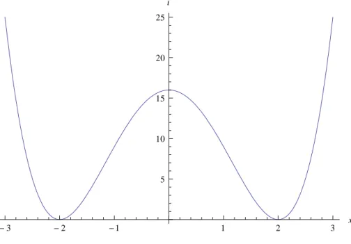
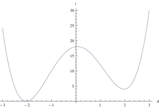
discussion here we choose the “the double-well potential”
G(y) = (y2−a2)2, (1.1.3) wherea >0. In Chapter 3 other forms ofGare considered as well.
Independent Brownian motions
First we consider independent standard Brownian motions on R indexed by the vertices
of the complete graph Kn starting from the mean-field measure µFn. At the level of the
empirical average this dynamics corresponds to a Brownian motion with small variance
(average ofnindependent Brownian motions). With this dynamics and the above choice of
Gwe prove that there is a critical time Tcrit with
Tcrit = 1
such that
(
there is a unique optimal trajectory if T ≤Tcrit there are multiple optimal trajectories if T > Tcrit,
and that there is only one bad empirical averageb= 0 whenT > Tcrit. Here the “badness”is
in the following sense. {mn(t)}n∈N denoting a sequence of stochastic processes for the empirical average, we say that a point b ∈ R is a bad at time T if the following two conditions hold:
1. Conditional onmn(T) = b,mn(0) does not converge (as n→ ∞) to a point-mass in distribution.
2. There exist two sequences b+k → b, b−k → b and δ > 0 such that the variational dis-tance between the distributionµ(0, T;b+k) of mn(0)|mn(T) =b+k and the distribution
µ(0, T;b−k) of mn(0)|mn(T) =b−k is at least δ for klarge enough.
ThusTcritis the time before which the transformed measureµ0T is Gibbs and after which it is non-Gibbs, where Gibbs/non-Gibbs is in the mean-field sense originally introduced in
[34]. Up to timeTcrit all empirical averages are good and afterTcrit,b= 0 becomes the only
bad empirical average. The above result extends to Brownian motions with constant drift
V. In this general context the critical time remains the same and after the critical time
there is a time-dependent bad empirical average b. This is unique for each time instance
and is given by b=V T, for anyT > Tcrit.
Ornstein-Uhlenbeck process
Second we apply an Ornstein-Uhlenbeck dynamics to the empirical average with µF n as the starting distribution.
Then the time-evolved measureµ0T is the projection at timeT of the law of the solution to the stochastic differential equation
dXtn= (−κXt+E)dt+ 1
√
ndBt, (1.1.5)
whereκ andEare real-valued parameters andBtis the standard Brownian motion. This is
a generalization of the previous dynamics in the sense that here we consider non-constant
drift. Under this dynamics we have a critical time
Tcrit = 1 2κlog
1 + κ
2a2
below and on which there is always a unique optimal trajectory, i.e. the time evolved
measure is Gibbs and above which there are multiple trajectories associated with the time
dependent bad empirical average
b= E
κ(1−e
−κT). (1.1.7)
At any time instance beyondTcrit, theb above is the only bad empirical average.
If the drift term −κXt+E in (1.1.5) is replaced by a general drift termf(Xt), wheref is an odd function and satisfies some other regularity conditions, then we can also show that
for short times the time evolved measure is Gibbs and becomes non-Gibbs at later times.
We have in this case no explicit expression for the critical time but we know the empirical
average b= 0 is bad (possibly other bad configurations can exist in this case).
Birth and death process
Further, we consider birth and death dynamics of the empirical average starting from µFn,
i.e., we consider a continuous time random walkXtnonRwith initial distributionµFn which makes jumps of size ±1/n at rates nb(x), resp.nd(x). For constant birth and death rates
band d, we obtain the same results as in the case of Brownian motion with constant drift.
Note that the case we choose the birth and death rates tob(x) =γ(1−x) andd(x) = (1+x), with x ∈ [−1,1] and γ ≥ 1, corresponds to the independent spin-flip dynamics (with an external field) of the empirical average of Ising spins. In this case we obtain, by analogy
with the case of the Ornstein-Uhlenbeck process, that at short time the system stays Gibbs
and becomes non-Gibbs at later time with time dependent bad empirical average
b= γ−1
γ+ 1
1−e−(1+γ)T
. (1.1.8)
Here, contrary to the Ornstein-Uhlenbeck case, we have no explicit expression for the critical
time.
The proofs of the above results use the Feng-Kurtz scheme [12, 18] to obtain a path-wise
large deviation rate functional for the constrained system. The optimal trajectories are then
obtained by minimizing this functional.
The rest of the thesis is organized as follows: In the rest of this chapter we collect the
tools that are used in the rest of the thesis. Chapter 2 contains the results for transforms of
one-dimensional Gibbs measures. The results on the dynamical Gibbs-non-Gibbs transitions
1.1.3 Large deviations for the trajectory of the empirical distribution and empirical measure
In Chapter 4 we compute the Feng-Kurtz Hamiltonian and Lagrangian associated to the
large deviations of the trajectory of the empirical distribution for independent Markov
pro-cesses, and of the empirical measure for translation invariant interacting Markov processes.
We treat both the case of jump processes (continuous-time Markov chains and interacting
particle systems) as well as diffusion processes. For diffusion processes, the Lagrangian is
a quadratic form of the deviation of the trajectory from the Kolmogorov forward equation.
In all cases, the Lagrangian can be interpreted as a relative entropy (density) per unit time.
1.2
Generalities on Gibbs and non-Gibbs measures
This section contains generalities on Gibbs and non-Gibbs measures. For more background
on Gibbs and non-Gibbs measures we refer the reader to [13, 19, 24, 39].
1.2.1 Gibbs measures
LetS be the single-site space, i.e. the set of all possible values for a spin. We assumeS is a
Polish space and is equipped with the Borel sigma algebraSassociated with the topology on
S. Mostly we considerS to be{−1,1}, a finite set,Ror an interval. TurnS into a measure
space by equipping it with an a priori measure ρ, usually a probability measure. Denote
by Ω = SZd the spin configuration space, describing all possible microscopic state of the
system, whereZdis thed-dimensional integer lattice withd≥1. Equip Ω with the product
topology and the product sigma algebra F =SZd. In what follows we will use upper case
Latin and Greek letters to represent subsets ofZd and lower case Latin and Greek letters
to denote elements in Ω.
For any subset Λ ⊆ Zd, denote by F
Λ the sigma algebra generated by the spins in Λ.
Denote by L the set of all finite subsets of Zd. For σ ∈ Ω and Λ ∈ L, we denote by σΛ
the restriction ofσ to Λ. A bounded measurable functionf : Ω→R is called local if there exists some ∆∈Lsuch thatf isF∆-measurable. The functionf is said to bequasilocal if
it is a uniform limit of local functions.
Potential and Hamiltonian
Definition 1.2.1. A potential is a function Φ : L×Ω → R such that Φ(Λ, .) is FΛ
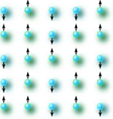
Figure 1.2: Ising model, the most well-known lattice-spin model, on a 2-dimensional lattice
convergent (UAC) if for all x∈Zd X
A3x
kΦ(A, σ)k∞<∞, (1.2.1)
where kΦ(A, σ)k∞= supσ∈Ω|Φ(A, σ)|.
Example 1.2.1. The family Φ given by
ΦA=
−J σxσy if |x−y|= 1 and A={x, y}
−hσx if x=y 0 otherwise,
(1.2.2)
where S ={−1,+1} and J >0, h ∈R. J is called the interaction strength and h is the external magnetic field. This interaction gives rise to the Ising model [32] for
ferromag-netism. It is one of the most studied statistical mechanical models. This is a lattice spin model for studying the phenomenon of ferromagnetism, i.e. it is a model for studying why
at low temperatures a piece of iron metal will continue to be magnetized even after a source of external magnetic field that it was in contact with is withdrawn. This phenomenon was believed to be associated with the alignment of the magnetic moments of the atoms. The
Ising model is a very simplified model where a magnetic moment is allowed to take two dif-ferent directions, namely it can point up (+1) or down (−1). See Figure 1.2 for an example of an Ising spin configuration in two dimensions. Note that the Ising potential is also UAC.
Definition 1.2.2. For ζ ∈ Ω and Λ ∈ L, the finite-volume Hamiltonian corresponding to potential Φ and with boundary condition ζ is defined as
HΛΦ,ζ(σ) = X AT
Λ6=∅
Φ(A, σΛζΛc), σ∈Ω, (1.2.3)
where σΛζΛc is the configuration in Ω that coincides with σ on Λ and coincides with ζ on Λc.
Remark 1.2.1. Note that HΛΦ,ζ is well-defined and is quasilocal as a function of ζ if Φ is
Finite/infinite-volume Gibbs measures and the DLR equations
Definition 1.2.3. For any potentialΦsatisfying 1.2.1 the finite-volume Gibbs measureµΦΛ,ζ associated with Λ∈L, the boundary condition ζ and temperature T = 1/β is given by
µΦΛ,β,ζ(dσ) =
exp−βHΛΦ,ζ(σ)
ZΛζ
Y
i∈Λ
ρ(dσi), (1.2.4)
where ZΛζ is the normalizing partition sum. The family γΦ = {µΛΦ,ζ,β, ζ ∈ Ω,Λ ∈ L} of finite-volume Gibbs measures is called a Gibbs specification.
Remark 1.2.2. For any UAC potential Φ, the familyγΦ is quasilocal, meaning that for any bounded quasilocal functionf, on Ω, and any Λ∈L
lim
∆↑Zdη,ζsup∈Ω; µ
Φ,η∆ζ∆c
Λ,β (f)−µ
Φ,η
Λ,β(f)
= 0, (1.2.5)
i.e. the expectation w.r.t. µΦΛ,·,β of a quasilocal function is again quasilocal, for all Λ∈L. Definition 1.2.4. A probability measure µ on Ωis called a Gibbs measure associated with
a UAC potential Φ, ρ and β if γΦ is a version of its conditional probabilities, i.e. for any
Λ∈L and bounded F-measurable function f on Ω
µ(f|FΛc)(·) =µΦ,·
Λ,β(f), µ−a.s.. (1.2.6)
The measure µ with the above property is said to be compatible with (or admitted by)γΦ.
The equations (1.2.6) are called theDLR equations, after Dobrushin, Lanford and Ruelle
[8, 9, 37].
Existence and uniqueness of Gibbs measure
We denote byG(γΦ) the set of Gibbs measures admitted byγΦ. If the single-site spaceS is
finite (and thus compact), its follows from the general weak convergence properties that for
every net of finite-volume Gibbs measures with boundary condition has a subnet with an
accumulation point. Further, if the associated specification is quasilocal, the accumulation
point is a Gibbs measure by the DLR equations. This also implies that the cardinality of
G(γΦ) is at least one forγΦ associated with a UAC interaction.
Next, for a quasilocal specification γΦ, the cardinality of G(γΦ) is exactly one in the
following scenarios:
1. There is no interaction among the spins. This occurs when β is zero or when Φ is
2. When the specification γΦ satisfies Dobrushin’s condition, see [24] Section 8.1. In
this case either there is small interaction among the spins and the Gibbs measure is
a small perturbation from a product measure or there is a very strong external field.
3. For one-dimensional lattice models, if the potential Φ satisfies
∞ X
n=0
f(n)<∞ (1.2.7) where
f(K) = sup i∈Z
X
A3i,diam(A)≥K
kΦ(A, σ)k∞, (1.2.8) then γΦ admits a unique Gibbs measure, see [24] Section 8.3. The one-dimensional
Ising model and one-dimensional lattice-spin models with finite range interaction
clearly belong to this family. The long-range Ising potential
Φ({i, j}, σ) = σiσj
|j−i|γ (1.2.9) also belongs to this family when γ > 2 (γΦ admits in fact multiple Gibbs measures
when γ ∈(1,2]).
Non-uniqueness of Gibbs measure
The existence of more than one Gibbs measure for γΦ, such as the one-dimensional
long-range Ising models (1.2.9) for γ ∈ (1,2] or the nearest neighbor Ising models (1.2.2) of dimension higher than one with low temperature, corresponds to the occurrence of a
first-order phase transition.
Let’s look at an example of γΦ that admits multiple Gibbs measures. The example we
consider here is the γΦ associated with the Ising interaction (1.2.2). The one-dimensional
version of this model, as we saw above, admits a unique Gibbs measure. This was the
case Ising treated in his PhD. Thesis. The original goal of Ising and his adviser Lenz was
to show that at low temperatures the magnetization of their model as a function of the
external fieldh behaves discontinuously at h= 0 (spontaneous magnetization), i.e., at low
temperatures a ferromagnetic substance will retain a net magnetization oriented in the
direction of the external field it is contact with even if this external source is turned off.
To the disappointment of Ising this behavior was absent in the one-dimensional case he
considered and he concluded this should be the case for models in dimensions higher than
one.
R.E. Peierls [46] gave an argument that disproved the claim for dimensions higher than
considers the case h = 0. The heuristic argument behind the proof is that at low
temper-atures the Gibbs measures are supported on configurations that are small perturbations of
the configurations that minimize the Ising Hamiltonian (ground state). For h = 0 there
are two such configurations, namely the all plus (+1) and the all minus (-1) configurations.
Therefore, if µ+ is a Gibbs measure obtained from a weak limit along a net of elements
inγΦ with the all plus (+1) boundary condition, then this measure will remember that it
came from a net of finite-volume Gibbs measures with all plus boundary condition. That is
the expected value of the spin at the origin is positive, even after taking the infinite-volume
limit. Similarly, ifµ− is constructed as above from an all minus (-1) boundary condition, it will also give a negative expected value to the spin at the origin. This implies that at low
enough temperatures there exist at least two Gibbs measures admitted by γΦ, one
nega-tively magnetized and the other posinega-tively magnetized. For instance, theµ+ measure lives
on configurations that are a sea of +’s with islands of minuses. In the Peierls argument the
sites that are of interest, as far as the Hamiltonian is concerned, are those pairs of sites with
misaligned spins. These sites serve as the boundary sites for an island of minuses. Such
sites determine a (d−1)-dimensional connected surfaces. Each such connected surface is called acontour. Each spin configuration corresponds uniquely (up to simultaneous flipping
of all spins) to a family of contours. The Peierls argument, essentially shows that under
µ+ at low enough temperatures, the probability of having a finite contour surrounding the
origin is strictly less than one-half.
1.2.2 Transformation of Gibbs measures and phenomenon of non-Gibbsianness
A probability measure µ on Ω is said to benon-Gibbsian if there is no UAC potential for
which its conditional probabilities can be written in the form (1.2.6). This usually occurs
when the conditional distributions of µ do not satisfy (1.2.5). This means that there is a
so-calledbad configurationthat leads to the violation of (1.2.5). More precisely, in the case
that the single-site spaceS is compact, it is defined as follows.
Definition 1.2.5. A configuration η ∈ Ω is said to be bad for a probability measure µ if there exist >0 and x ∈Zd such that for all Λ ∈L, with x∈ Λ, there exist Γ⊃Λ, with
Γ∈L, such that:
sup ξ,ζ
µΓ(σx|ηΛ\{x}ξΓ\Λ)−µΓ(σx|ηΛ\{x}ζΓ\Λ)
> . (1.2.10)
This implies thatηis an essential point of discontinuity of every version of the conditional
probability ofµ(σx|(·)Zd\{x}).
Non-Gibbsian measures arise naturally from transformations of Gibbs measures as was
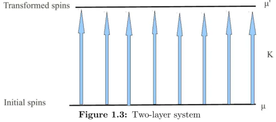
Figure 1.3: Two-layer system
1. Coarse-graining of initial lattice and projection of initial lattice to lower-dimensional
lattice as is done for renormalization group (RG) transformations such as block-spin
transformations, decimation transformations, Kadanoff transformations [3, 13, 27, 28,
29, 33].
2. Fuzzification or discretization of the initial spin space [14, 30, 50].
3. Stochastic time-evolution of Gibbs measures [6, 11, 15, 16, 40, 45, 47].
In all these transformations the Gibbs property of the initial system is for some times
conserved and for other times lost.
1.2.3 The two-layer picture
Consider a Gibbs measureµfor an initial spin system and then generate a new probability
measure µ0 by applying a probability kernelK toµ,
µ0(ω0) = (µK)(ω0)≡X
ω
µ(ω)K(ω→ω0). (1.2.11)
µ and µ0 need not live on the same configuration space. To prove that the transformed measureµ0 is Gibbs or not one usually considers the so-called two-layer system ¯µconsisting of the initial spins, that are distributed according to µ, and the transformed spins. The
initial and the transformed spins are coupled together byK in such a way that the marginal
of this joint distribution to the transformed spins isµ0, see Figure 1.3.
The problem of checking whether µ0 is Gibbs or not reduces to the problem of checking whether the constrained system ¯µ[η], i.e. the joint system constrained to configurations
Ωη × {η} where Ωη is the set of those initial spins that are mapped to η by K, exhibits phase transitions or not. If the constrained system has a unique Gibbs measure uniformly
inη, thenµ0 is Gibbs andµ0 is non-Gibbs otherwise.
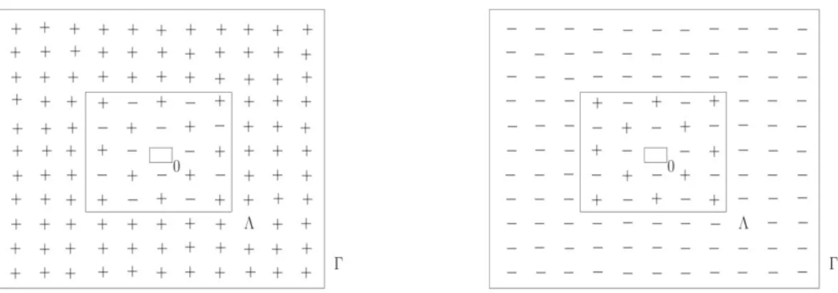
Figure 1.4: A plus-minus alternating configuration approximated with the all-plus boundary (left) and approximated with the all-minus boundary (right).
Example 1.2.2. Letµ+be the plus phase for thed-dimensional Ising at low enough temper-ature. Starting from µ+, Van Enter, Fernandez, den Hollander and Redig [11], considered
infinite/high temperature spin-flip dynamics of the initial spins towards a reversible Gibbs measure. Under this dynamics the time-evolved measure µ+t was shown to be Gibbs for
short times and non-Gibbs at later times. In the case there is a small positive external field the measure becomes Gibbs again at large but finite times. For the case of zero external field for the initial system the Gibbs property is lost forever.
The intuitive argument for these Gibbs-non-Gibbs transitions is as follows: The
con-strained system can be viewed as the initial system with a dynamical external field. This field is generated by the constraint on the second layer. For short times this field is very
strong and forces the constrained system to be in the uniqueness regime. The strength of the field decays to zero as time goes to infinity. If we start with an initial system with zero external field, then at large enough times there will be configurations that are neutral
with respect to the all-plus boundary and the all-minus boundary, such as a plus-minus alternating configuration (see Figure 1.4), meaning there exists a phase transition for the constrained system. On the other hand, if the initial system has non-zero initial field, we
can choose the constrained second-layer configuration in such a way that in an intermediate range of times the dynamical field cancels the initial field in the constrained system. This
will cause the constrained system to exhibit a phase transition if the temperature is low enough. But if we wait long enough the dynamical field will fade away giving way to the initial field to once again force the constrained system into the uniqueness regime.
Example 1.2.3. Next we consider the decimation transformation of the 2-dimensional Ising model [13, 38]. The decimation transformation K with spacing 2 maps the configuration
space Ω onto itself in the following sense: For any initial configuration ω ∈Ω, ω0 =Kω is such thatω0x=ω2x, forx∈Z. Then, as before, we apply the decimation transformation to a
Gibbs measureµof a low-temperature Ising model. Note that here the transformed spins live
initial spin system. The constrained system associated with the transformed configuration
ω0 lives onZ2 but is supported on the configurations with all spins in 2Z2 fixed to ω0. For
an initial Ising model at low enough temperature and in zero field, the constrained system associated with a plus-minus alternating configuration (bad configuration) admits multiple
Gibbs measures and the decimated measure becomes non-Gibbs. In the case we start with initial Ising model at low enough temperature and in non-zero field, it is shown that
a bad configuration, different from the plus-minus alternating configuration, is needed to ’annihilate’ the initial external field to force the constrained system into the phase transition regime.
1.3
Large deviation theory and optimal solutions for rate
function
In this section we collect some results from the theory of large deviations. Large deviation
theory deals with deviations, of certain random objects, larger than those captured by the
central limit theorem.
1.3.1 Large deviation principle
Here we collect some general notions for large deviations. For more background on large
deviations, we refer the reader to [5, 10, 31]. Let X be a Polish space, i.e. a complete
separable metric space.
Definition 1.3.1. The function I :X7→[0,∞]is called a rate function if 1. I 6=∞,
2. I is lower semi-continuous,
3. I has compact level sets.
Definition 1.3.2. A sequence of probability measures (Pn)n∈N on X satisfies the large deviation principle (LDP) with raten and with rate function I if
1. I is a rate function in the sense of Definition 1.3.1,
2. lim supn→∞n1 logPn(C)≤ −I(C) ∀C⊆Xclosed,
Let us now discuss some examples of sequences of probability measures that will appear
in the later part of the thesis. Consider the sequence X= (Xn)n∈N of real-valued
indepen-dent and iindepen-dentically distributed random variables with common law ρ. The first result is
Cram´er’s Theorem [4], for the sequence of probability measures (Pn)n∈N, where Pn is the
law of theempirical average
L(1)n = 1
n
n X
i=1
Xi. (1.3.1)
Theorem 1.3.3 (Cram´er’s Theorem). Let Pn be as above and suppose that
ϕ(t) = Z
R
etxρ(dx)<∞, for any t∈R. (1.3.2)
Then the sequence of probability measures (Pn)n∈N onX satisfies the LDP with rate n and
with rate function
I(z) = sup t∈R
[zt−logϕ(t)], z∈R. (1.3.3) This result is usually called the level-one LDP. Note that hereXis R. For the caseρ is
the standard Gaussian the rate function becomes
I(z) = z
2
2 , z∈R. (1.3.4)
Next we look at the sequence (Pn)n∈N, wherePnis the law of theempirical distribution
L(2)n = 1
n
n X
i=1
δXi, (1.3.5)
where δx is the point-mass at x ∈ R. L(2)n is a random probability measure on R. The
large deviation principle in this case is called Sanov’s Theorem [48]. This is also called the
level-two LDP. Note that Xhere is the set of probability measures on R.
Theorem 1.3.4 (Sanov’s Theorem). The sequence(Pn)n∈N, of the law of the empirical distribution satisfies the LDP on X with rate nand rate function
Iρ(ν) = ( R
Rν(dx) log
dν dρ(x)
, if νρ
∞ otherwise, (1.3.6)
where dνdρ(x) is the Radon-Nikodym derivative of ν with respect to ρ and ν ρ means ν is absolutely continuous with respect to ρ.
LetX(n) = (X1, X2,· · · , Xn)per be the periodic extension of the vector (X1, X2,· · ·, Xn) to an element in RN. Consider the sequence (Pn)n∈N of probability measures on X, where
Pnis the law of theempirical measure
L(3)n = 1
n
n X
i=1
δτiX(n), (1.3.7)
where τ is the left shift operator acting on RN. In this case X is the set of probability
measures on RN invariant under τ. For any element µ of X the specific relative entropy
H(µ|ρN) ofµw.r.t. ρN is defined as
H(µ|ρN) = lim
N→∞ 1
Nh(πNµ|ρ
N), (1.3.8)
whereπNµis the projection ofµonto the first N coordinates.
Theorem 1.3.5. The sequence (Pn)n∈N of the laws of the empirical measure satisfies the LDP on X with raten and rate function
Iρ∞(µ) =H(µ|ρN). (1.3.9)
See [5] Section 6.5.3 for a proof of this theorem. There is an analogous version of
Theorem 1.3.5 if the initial sequence X of random variables is replaced by a family of
random variables indexed by Zd. Here we consider a net of probability measures indexed
by progressively increasing subsets ofZd that exhaustZd. This net of subsets must have a
surface–volume ratio that tends to zero. This property is called thevan Hoveproperty. An
example of such a net is the net of boxes Λn ={−n,−n+ 1,· · · , n−1, n}d. In this case the empirical measure becomes
¯
L(3)n = 1
|Λn|
X
x∈Λn
δΘxX(n), (1.3.10)
where |Λn| is the cardinality of Λn, Θx is the translation of points in Zd by x and X(n) is
the periodic extension of elements in RΛn to points in RZ
d
. With this choice the LDP rate
is|Λn|andXis the space of all translation invariant probability measures onRZd. Further,
Pnis the law of ¯L(3)n . The specific relative entropy for µinXw.r.t. ρZ d
becomes
H(µ|ρZd) = lim Λ↑Zd
1
|Λ|h(πΛµ|ρ
Λ), (1.3.11)
where πΛµis the projection of µ onto the coordinates in Λ and the limit is along a net of
subsets ofZd that has the van Hove property.
Next we review the tilted LDP. Given a sequence (net) of probability measures satisfying
the LDP, the tilted LDP allows us to generate a new sequence (net) of probability measures
that also satisfies the LDP. This is achieved by tilting the original sequence with exponential
Theorem 1.3.6 (Tilted LDP). Let (Pn)n∈N satisfy the LDP on X with rate n and with
rate functionI. LetF :X→Rbe a continuous function that is bounded from above. Define
Jn(S) = Z
S
enF(x)Pn(dx), with S∈X Borel. (1.3.12)
Then the sequence (PnF)n∈N of probability measures, defined by
PnF(S) = Jn(S)
Jn(X), with S ∈X Borel, (1.3.13)
satisfies the LDP on Xwith rate n and with rate function
IF(x) = sup y∈X
[F(y)−I(y)]−[F(x)−I(x)]. (1.3.14) See [10] Section II.7 for a proof of this theorem.
1.3.2 Large deviations for stochastic processes
In this subsection we give LDPs for Brownian motion with small variance and Itˆo diffusion
with small variance. These are LDPs for sequences of probability measures living on the
space of paths. The standard Brownian motion result is called Schilder’s Theorem [49].
This gives an estimate for the probability that a sample path of Brownian motion with
small variance will stray far from the mean path. In this section the space X is the the
Banach spaceC0 of continuous functionsf : [0, T]→Rd such thatf(0) = 0, equipped with
the supremum norm.
Theorem 1.3.7 (Schilder’s Theorem). Let B be a standard d-dimensional Brownian motion starting at the origin. LetP denote the law ofB, i.e., the classical Wiener measure. For n ∈ N, let Pn denote the law of the rescaled process B/
√
n. Then, the sequence of
probability measures (Pn)n∈N satisfies the LDP onXwith rate nand rate functionI :C0 →
R∪ {+∞}given by
I(ω) = ( 1
2
RT
0 |ω˙(t)|
2dt if ω
t is absolute continuous
+∞ otherwise. (1.3.15)
We now present the Freidlin-Wentzell Theorem [22] which extends the Schilder’s
Theo-rem to Itˆo diffusion with small variance.
Theorem 1.3.8 (Freidlin-Wentzell Theorem). Let B be a standard d-dimensional Brownian motion starting at the origin. For n ∈ N, let Pn be the law of the solution
Xn of the Itˆo stochastic differential equation
(
dXtn=b(Xtn)dt+√1 ndBt
where the drift vector field b : Rd → Rd is uniformly Lipschitz continuous. Then, the
se-quence of probability measures(Pn)n∈N satisfies the LDP onXwith ratenand rate function
I(ω) = (
1 2
RT
0 |ω˙t−b(ωt)|
2dt if ω lies in the Sobolev spaceH1([0, T];
Rd)
+∞ otherwise. (1.3.17)
1.3.3 The Feng-Kurtz scheme
In this section we review the Feng-Kurtz scheme [18] (Example 1.5) for studying the large
deviation properties for the trajectories of more general Markov processes. We follow closely
Appendix A.2 of [12] to explain this scheme as follows.
Consider a sequence of Markov processes X = (Xn)n∈N with Xn = {Xn(t)}t≥0, living
on a common state space (likeR,Rdor a space of probability measures). Suppose thatXn has generatorLn and in the limit asn→ ∞converges to a process (x(t))t≥0, which can be
either deterministic or stochastic. Then, by the Markov property, if the sequencePn of the
laws of Xn satisfies the LDP, then the rate function takes the form
¯
I(γ) = Z T
0
L(γt,γ˙t)dt, (1.3.18)
where the functiont7→L(γt,γ˙t) is called the ’Lagrangian’ and the dot above γt means the derivative with respect to time. The Feng-Kurtz scheme provides a procedure to identify
the Lagrangian. We outline the scheme in following four steps:
1. Compute the generator of the non-linear semigroup
(Hf)(x) = lim n→∞
1
ne
−nf(x) L
nenf
(x). (1.3.19)
2. Look for a function H(x, p) of two variables such that
(Hf)(x) =H(x,∇f(x)). (1.3.20) What ∇f means depends on the context: on Rd it simply is the gradient off, while
on an infinite-dimensional state space it is a functional derivative.
3. The LagrangianL is obtained as the Legendre transform ofH:
L(x, λ) = sup p
[hp, λi −H(x, p)]. (1.3.21) What h·i means also depends on the context: on Rd it simply is the inner product,
while in general it is a natural pairing between a space and its dual, such ashf, µi= R
4. The Lagrangian in (1.3.18) is the functionL withx=γtand λ= ˙γt.
The LagrangianL(x,x˙) is exactly the Lagrangian inLagrangian mechanics, withxbeing
interpreted as the (generalized) position and ˙x as the (generalized) velocity. The function
H(x, p) is called the ’Hamiltonian’. It is exactly the Hamiltonian inHamiltonian mechanics,
withxbeing interpreted as the (generalized) position andpas the (generalized) momentum,
but is a completely different object than the spin (e.g. Ising) Hamiltonian. For background
of Lagrangian and Hamiltonian mechanics, we refer the reader to [25].
All the above LDP results assume the process starts from a fixed point, say the origin.
The question now is “Will these results continue to be true if we start from a randomly
chosen point?”. This question is answered in the affirmative. The only thing that changes
is the rate function. In particular, if the sequence of Markov processesX = (Xn)n∈N, with
Xn={Xn(t)}t≥0, start from the sequence of initial distributions (µn)n∈N that satisfies the
LDP with rate nand rate function I. Then the sequence X = (Xn)n∈N satisfies the LDP
with rate nand rate function
I(γ) =I(γ0) +
Z T
0
L(γt,γ˙t)dt. (1.3.22)
For details, see Feng and Kurtz [18].
1.3.4 Uniqueness and non-uniqueness of optimal trajectories
From Lagrangian mechanics the rate functional ¯I(1.3.18) is theaction functional associated
with the LagrangianL(1.3.21). The natural question that comes to mind is “What are the
trajectories that give rise to the least action?”. Such trajectories with least action are the
solutions of the Lagrange equations
d dt
∂L ∂x˙t
= ∂L
∂xt
(1.3.23)
or, equivalently, the Hamilton equations
˙
xt=
∂H ∂pt
, p˙t=−
∂H ∂xt
. (1.3.24)
For the action functionalI (1.3.22), the optimal trajectories have to satisfy theopen-start
condition
∂L(xt,x˙t)
∂x˙t
t=0
=
∂I(x0)
∂x0
x0=a
(1.3.25)
in addition to the above Lagrange’s equation.
For the applications in this thesis, we want optimal trajectories associated with the rate
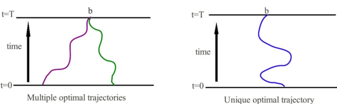
Figure 1.5: Optimal trajectories for path-wise constrained system
at a fixed terminal point. This path measure is what we called the constrained system.
The trajectories we consider include trajectories of empirical average (real-valued) (1.3.1),
empirical distribution (probability measure on the single-spin spaceS) (1.3.5) and empirical
measure (probability measure on the configuration space Ω) (1.3.7) of configurations of spin
systems. The starting configuration of the spin system will be chosen according to a Gibbs
measure. The question now is whether the time-evolved measure, on the spin configurations,
retains or loses its Gibbs property. The answer to this question is linked to the existence
of multiple optimal trajectories for the large deviation rate functional for the constrained
system. If there is a unique optimal trajectory connecting any fixed terminal point at time
T > 0 to a point at time zero then the time-evolved measure at time T is Gibbs. On the
other hand, if there are multiple optimal trajectories associated to some fixed terminal point
b at time T >0, then the time-evolved measure at time T is non-Gibbs and the terminal
point b is said to be bad. This is analogous to the two-layer approach for studying
Gibb-non-Gibbs properties of transforms of Gibbs measures. Uniqueness of optimal trajectory
corresponds, in the two-layer picture, to uniqueness of the constrained system. Multiplicity
of optimal trajectories corresponds to the occurrence of phase transitions in the constrained
[1] A. Bovier, Statistical mechanics of disordered systems, a mathematical perspective,
Cambridge University Press, New York (2006).
[2] X. Bressaud, R. Fern´andez, A. Galves, Decay of correlations for non H¨olderian
dynam-ics, A coupling approach, Electr. J. Prob.,4, 1–19 (1999).
[3] J. Bricmont, A. Kupiainen, R. Lefevere, Renormalization group pathologies and the
definition of Gibbs states. Comm. Math. Phys.,194, 359–388 (1998).
[4] H. Cram´er, Sur un nouveau theoreme-limite de la theorie des probabilites, Actualites
Scientifiques et Industrielles, 736, 5–23, Hermann, Paris (1938).
[5] A. Dembo, O. Zeitouni, Large deviations techniques and applications, Second edition,
Springer Verlag (2010).
[6] D. Dereudre, S. Roelly, Propagation of Gibbsianness for infinite-dimensional gradient
Brownian diffusions, J. Stat. Phys.,121, 511–551 (2005).
[7] R.L. Dobrushin, Existence of a phase transition in the two-dimensional and
three-dimensional Ising models, Soviet Physics Dokl.,10, 111–13, (1965).
[8] R.L. Dobrushin, The description of a random field by means of conditional probabilities
and conditions of its regularity, Theor. Prob. Appl.,13, 197–224 (1968).
[9] R.L. Dobrushin, Definition of a system of random variables by means of conditional
distributions, Teor. Verojatnost, i Primenen., 15, 469–497 (1970).
[10] R.S. Ellis, Entropy, large deviations and statistical mechanics, Springer, New York
(1985).
[11] A.C.D. van Enter, R. Fern´andez, F. den Hollander, F. Redig, Possible loss and recovery
of Gibbsianness during the stochastic evolution of Gibbs Measures, Commun. Math.
[12] A.C.D. van Enter, R. Fern´andez, F. den Hollander, F. Redig, A large-deviation view
on dynamical Gibbs-non-Gibbs transitions, Mosc. Math. J.,10, 687–711 (2010).
[13] A.C.D. van Enter, R. Fern´andez, A. Sokal, Regularity properties and pathologies of
position-space renormalization-group transformations: scope and limitations of
Gibb-sian theory, J. Statist. Phys.,72, 879–1167 (1993).
[14] A.C.D. van Enter, C. Kuelske, A.A. Opoku, Discrete approximations to vector spin
models. J. Phys. A,44(2011).
[15] A.C.D. van Enter, C. K¨ulske, A.A. Opoku and W.M. Ruszel, Gibbs-non-Gibbs
prop-erties forn-vector lattice and mean field models, Braz. J. Probab. Stat., 24, 226–255
(2010).
[16] A.C.D. van Enter, W.M. Ruszel, Gibbsianness versus non-Gibbsianness of time-evolved
planar rotor models, Stoch. Proc. Appl.119, 1866–1888 (2009).
[17] V. Ermolaev, C. K¨ulske, Low-temperature dynamics of the Curie-Weiss model: periodic
orbits, multiple histories, and loss of Gibbsianness, J. Stat. Phys.,141, 727–756 (2010).
[18] J. Feng, T.G. Kurtz, Large Deviations for Stochastic Processes, American
Mathemat-ical Society, Providence RI (2006).
[19] R. Fern´andezGibbsianness and non-Gibbsianness in lattice random fields, Les Houches,
LXXXIII (2006).
[20] H. F¨ollmer, Random economies with interacting systems, J. Math. Econ., 1, 51–62
(1974).
[21] R. Fern´andez, F. den Hollander, J. Martinez, Variational description of
Gibbs-non-Gibbs dynamical transitions for the Curie-Weiss model, arXiv:1202.4205v2 (2012)
[22] M.I. Freidlin and A.D. Wentzell, Random perturbations of dynamical systems,
Grundlehren der Mathematischen Wissenschaften [Fundamental Principles of
Math-ematical Sciences]260, (2nd edition), Springer-Verlag, New York, pp. xii+430 (1998)
[23] S. Geman, D. Geman, Stochastic Relaxation, Gibbs Distributions, and the Bayesian
Restoration of Images, IEEE Trans. PAMI6, 721–741 (1984).
[24] H.O. Georgii,Gibbs measures and phase transitions, (2nd edition), de Gruyter, Berlin
[25] H. Goldstein, C.P. Poole, J.L. Safko,Classical mechanics (3rd edition), Addison Wesley
(2002).
[26] R.B. Grifths, Peierls proof of spontaneous magnetization in a two-dimensional Ising
ferromagnet. Phys. Rev. (2),136, A437–9 (1964).
[27] R.B. Griffiths, P.A. Pearce, Position-Space Renormalization-Group Transformations:
Some Proofs and Some Problems, Phys. Rev. Lett.,41, 917–920 (1978).
[28] R.B. Griffiths, P.A. Pearce, Mathematical properties of position-space
renormalization-group transformations, J. Stat. Phys.,20, 499–545 (1979).
[29] R.B. Griffiths, Mathematical properties of renormalization-group transformations,
Physica, 106A, 59–69 (1981).
[30] O. Haggstrom, Is the fuzzy Potts model Gibbsian?, Ann. de Institut Henri Poincare
(B) Prob. and Stat.,39, 891–917 (2003).
[31] F. den Hollander,Large deviations, Fields Institute Monographs, American
Mathemat-ical Society (2008).
[32] E. Ising, Beitrag sur Theorie des Ferromagnetismus, Zeit. fur Physik, 31, 253–258
(1925).
[33] R.B. Israel, Banach algebras and Kadanoff transformations, In Random Fields -
Rigor-ous Results in Statistical Mechanics and Quantum Field Theory, Vol. II., Coll. Math.
Soc., Janos Bolyai,27, 593–608, North-Holland, Amsterdam (1979).
[34] C. K¨ulske, A. Le Ny, Spin-flip dynamics of the Curie-Weiss model: Loss of Gibbsianness
with possibly broken symmetry, Comm. Math. Phys., 271, 431–454 (2007).
[35] C. K¨ulske and A.A. Opoku, The posterior metric and the goodness of Gibbsianness for
transforms of Gibbs measures, Electron. J. Probab.,13, 1307–1344 (2008).
[36] C. K¨ulske, A. Opoku, Continuous spin mean-field models: limiting kernels and Gibbs
properties of local transforms, J. Math. Phys., 49, 125215 (2008).
[37] O.E. Lanford, D. Ruelle, Observables at infinity and states with short range correlations
in statistical mechanics, Comm. Math. Phys.,13, 194–215 (1969).
[38] A. Le Ny, Decimation on the two-dimensional Ising model: non-Gibbsianness at low
temperature. Almost Gibbsianness or weak Gibbsianness?, Publ. Inst. Rech. Math.
[39] A. Le Ny, Introduction to (generalized) Gibbs measures, Ensaios Matem´aticos,
So-ciedade Brasileira de Matem´atica, Rio de Janeiro,15, 1-126 (2008).
[40] A. Le Ny, F. Redig, Short-time conservation of Gibbsianness under local stochastic
evolutions, J. Stat. Phys.,109, 1073–1090 (2002).
[41] C. Maes, K. van de Velde, Defining relative energies for the projected Ising measure,
Helv. Phys. Acta.,65, 1055–1068 (1992).
[42] C. Maes, K. van de Velde, The interaction potential of the stationary measure of a
high-noise spin-flip process, J. Math. Phys.,34, 3030–3038 (1993).
[43] C. Maes, F. Redig, A. van Moffaert, The restriction of the Ising model to a layer, J.
Stat. Phys.,96, 67–107 (1999).
[44] C. Maes, F. Redig, A. van Moffaert, Potentials for one-dimensional restrictions of
Gibbs measures, in Mathematical results in statistical mechanics, eds. S. Miracle-Sol´e,
J. Ruiz, V. Zagrebnov, World Scientific (1999).
[45] A.A. Opoku,On Gibbs properties of transforms of lattice and mean-field systems, PhD
thesis, Rijksuniversiteit Groningen (2009).
[46] R.E. Peierls, On Ising’s ferromagnet model, Proc. Camb. Phil. Soc.,32, 477–481 (1936).
[47] W.M. Ruszel, Gibbs and Non-Gibbs Aspects of Continuous Spin Models, PhD thesis,
Rijksuniversiteit Groningen (2010).
[48] I.N. Sanov, On the probability of large deviations of random variables, Mat. Sb., 42
(in Russian), English translation in: Selected translations in mathematical statistics
and probability I, 213–244 (1961).
[49] M. Schilder, Some asymptotic formulae for Wiener integrals, Trans. Amer. Math. Soc,
125, 63–85 (1966).
[50] E. Verbitskiy, Variational principle for fuzzy Gibbs measures, Mosc. Math. J.,10, no.4,
Transformations of
one-dimensional Gibbs measures
with infinite-range interaction
2.1
Introduction
Local transformations of Gibbs measures can be non-Gibbs. In [1], the mechanism behind
the creation of non-Gibbsianness is explained as a hidden phase transition: conditioned
on a certain configuration of the transformed spins, the original spins can exhibit a phase
transition. Even if the untransformed system is not in a phase transition regime, by
condi-tioning on the transformed configuration we can bring it into a regime of phase transition.
In a regime of strong uniqueness, such as the Dobrushin uniqueness regime, or the
com-plete analyticity regime, one expects that Gibbs measures turn into Gibbs measures under
stochastic or deterministic disjoint-block transformations.
For one-dimensional systems in the uniqueness regime, one also expects that local
trans-formations conserve the Gibbs property. Using disagreement percolation, this has been
proved for finite-range potentials, [9]. The technique of disagreement percolation has
how-ever not been extended to the case of infinite range interactions, and in fact (at present)
breaks down in that context. Further, it is also known that in the uniqueness regime in
dimension one, decimating sufficiently many times brings the system into a regime where
cluster expansion can be obtained, and hence the system becomes completely analytic [3].
Finally, in the context of dyamical systems, it has been shown recently [4] that a Gibbs
measure with an exponentially decaying interaction transforms into a Gibbs measure with
“confuses” symbols (i.e., the transformed spin is determined by a partition of the
untrans-formed spin).
In this paper we consider lattice spin systems in one dimension, with an interaction that
is allowed to be of infinite range. We consider single-site stochastic and deterministic
trans-formations. We prove that under a uniqueness condition (see 2.2.8 below), the transformed
measure is Gibbs. We further prove that, if the initial interaction is exponentially
decay-ing, then the transformed interaction decays exponentially as well. If the initial interaction
decays (in some sense) as a power law with power α (which is chosen big enough to be in
the uniqueness regime), then the tranformed interaction can be estimated with a (smaller)
power as well.
The method of proof is based on two ingredients. One ingredient is classical: the
single-site conditional probabilities of the transformed measure can be written as the expected
value of a local function in a Gibbs measure that depends on the conditioning. The
de-pendence on the conditioning, in the case of a single-site transformation is in the form of
a spatially varying magnetic field. The second step is to control how the local function
expectation depends on this magnetic field. This reduces to the problem of how well a
lo-cal expectation is approximated by finite-volume Gibbs measure expectations (in a context
which is not spatially homogeneous because of the presence of the magnetic field
depend-ing on the conditiondepend-ing). In this second step we use coupldepend-ing, in the spirit of [2]. As a
consequence of this method, we obtain, besides Gibbsianness, estimates on the decay of
the transformed potential (where we use the so-called Kozlov potential defined on lattice
intervals).
Our paper is organized as follows: we start with basic definitions on Gibbs measures,
po-tentials, and define the transformations that we consider. Section 2.2 is devoted to the case
of stochastic single-site transformations. Section 2.3 contains the single-site deterministic
case.
2.2
Gibbs measures and their transformations
2.2.1 One-dimensional Gibbs measures
We consider lattice spin systems, with configuration Ω =SZ, whereS, the single-site space,
is a finite set. We equip Ω with the product topology. The set of all finite subsets of Z is
denoted by L. For Λ∈Land σ ∈Ω, we denote by σΛ the restriction of σ to Λ, while ΩΛ
A function f : Ω → R is called local if there exists a finite set ∆ ⊆ Z such that
f(η) =f(σ) for η and σ coinciding on ∆.
Continuity in the product topology coincides with quasi-locality, i.e., a functionf : Ω→
Ris continuous if and only if it is a uniform limit of local functions, more precisely if
lim
Λ↑Zξ,ζ∈supΩ|f(ωΛξΛ
c)−f(ωΛζΛc)|= 0, (2.2.1) Definition 2.2.1. A functionΦ :L×Ω→Rsuch thatΦ(A, σ)depends only onσ(x),x∈A
for∀A∈L, is called apotential. A potential isuniformly absolutely convergentif for allx∈Z
X
A3x
kΦ(A, σ)k∞<∞, (2.2.2)
where kΦ(A, σ)k∞= supσ∈Ω|Φ(A, σ)|.
For Φ ∈ B, ζ ∈ Ω, Λ ∈ L, we define the finite-volume Hamiltonian with boundary condition ζ as
HΛζ(σ) = X AT
Λ6=∅
Φ(A, σΛζΛc). (2.2.3)
Corresponding to this Hamiltonian we have thefinite-volume Gibbs measures µΦΛ,ζ, Λ∈L, with boundary condition ζ, defined on Ω by
Z
f(ξ)µΦΛ,ζ(dξ) = X σΛ∈ΩΛ
f(σΛζΛc)
exp−HΛζ(σ)
ZΛζ , (2.2.4)
where ZΛζ denotes the partition function normalizing µΦΛ,ζ to a probability measure and
f : Ω7→Rdenotes any local function. For a probability measure µon Ω, we denote by µζΛ
the condition probability distribution of σ(x), x ∈ Λ, givenσΛc = ζΛc, which is of course only µ−a.s. defined.
Definition 2.2.2. ForΦ∈B, we callµa Gibbs measurewith potential Φif a version of its conditional probabilities coincides with the ones prescribed in (2.2.4), i.e., if
µΦΛ,ζ =µζΛ µ−a.s. ∀Λ∈L, ζ ∈Ω. (2.2.5) We assume that the potential Φ satisfies the following condition.
sup i∈Z
X
A3i,diam(A)≥K
kΦ(A, σ)k∞=f(K) (2.2.6) wheref satisfies
∞ X
n=0
Under the condition 2.2.7, the potential Φ admits only one Gibbs measureµ=µΦ, see [5],
section 8.3. Condition 2.2.7 of course implies
lim k→∞
X
j≥0
f(j+k) = 0. (2.2.8)
We abbreviate
Fk= X
j≥0
2f(j+k) (2.2.9)
Remark that in the case of a translation invariant potential, the supremum in (2.2.6) can
be omitted and then
f(K) = X
A30,diam(A)≥K
kΦ(A, σ)k∞
Definition 2.2.3. A version of conditional probabilities {µ(·|ζΛc) : ζΛc ∈ ΩΛc,Λ ∈ L} is
called uniformly non null if for every Λ ∈L, there exists a constant mΛ >0 such that
for everyω ∈Ω
µωΛ(ω)≥mΛ. (2.2.10)
The following theorem due to Kozlov [7] and Sullivan [11] gives a criterion to decide
whether a given measure is Gibbsian.
Theorem 2.2.4. A probability measure µ on (Ω,F) is a Gibbs measure with respect to a
uniformly absolutely convergent potential iff there exists a version of its conditional proba-bilities that is continuous and uniformly non null.
Remark 1. Theorem 2.2.4 is constructive, i.e., the potential is constructed from the
con-ditional probabilities. See section 2.3.1 for the explicit form. In our one-dimensional case, it is non-vanishing on lattice intervals only, i.e., sets of the form [i, j] = {i, i+ 1, . . . , j}. Therefore, if we start from a Gibbs measure we can assume without loss of generality that
the potential is non-zero only on lattice intervals.
2.2.2 Transformations of Gibbs measures
We consider two types of transformation: site stochastic tranformations and
single-site deterministic transformations.
We first consider single-site stochastic transformation, i.e., for a givenσ, the distribution
of the image spin configuration is a product measure on (S0)Z
T(ξ|σ) =Y i∈Z
We assume that the transition kernel of a single site is strictly positive. That is, for
i∈Z,
inf
i∈Z,ξi,σiPi(ξi|σi)>0. (2.2.13) The distribution of the image spin is then defined as
µ◦T(dξ) = Z
T(dξ|σ)µ(dσ). (2.2.14)
The second case is a single-site deterministic transformation T : Ω→ Ω0 induced by a mapϕ:S→S0 given by
(T(σ))i=:σ0i=ϕ(σi) (2.2.15)
2.3
Stochastic single-site transformations
Theorem 2.3.1. For single site stochastic transformations, if the potentialΦcorresponding
to the initial Gibbs measure µ satisfies condition (2.2.6), (2.2.7), then the transformed measureµ◦T is a Gibbs measure.
Proof. First of all, {µ◦T(·|ζΛc) : ζΛc ∈ ΩΛc,Λ ∈ L} is uniformly non null thanks to the positivity assumption of a single site’s transformation kernel in (2.2.13). We then proceed with the proof in two steps.
First, we express the one-site conditional probabilities µ◦T(ξ0|ξZ\{0}) as averages of a local observable over a Gibbs measure depending on the conditioningξ. This is in the spirit of [8], but simpler since the transformation is stochastic, and hence the “constrained first
layer model” of [8] is “not constrained” (given the image configuration, all configurations are possible as originals).
Second, we use a “house-of-cards” coupling technique (see (2.3.7)) in the spirit of [2] to
prove the dependence of this local expectation on the conditioning ξ. We restrict to the conditional expectation of the transformed spin at the origin, given the transformed spins outside the origin. The same argument applies to conditional expectation of the spin at