The R Inferno

(1)

Patrick Burns

1

30th April 2011

1_{This document resides in the tutorial section of http://www.burns-stat.com. More}

(2)

List of Figures

2.1 The giants by Sandro Botticelli. . . 14

3.1 The hypocrites by Sandro Botticelli. . . 19

4.1 The panderers and seducers and the flatterers by Sandro Botticelli. 25 5.1 Stack of environments through time. . . 32

6.1 The sowers of discord by Sandro Botticelli. . . 36

7.1 The Simoniacs by Sandro Botticelli. . . 41

8.1 The falsifiers: alchemists by Sandro Botticelli. . . 47

8.2 The treacherous to kin and the treacherous to country by Sandro Botticelli. . . 81

8.3 The treacherous to country and the treacherous to guests and hosts by Sandro Botticelli. . . 103

9.1 The thieves by Sandro Botticelli. . . 116

(8)

List of Tables

2.1 Time in seconds of methods to create a sequence. . . 12

3.1 Summary of subscripting with 8[8. . . 20

4.1 The apply family of functions.. . . 24

5.1 Simple objects. . . 29

5.2 Some not so simple objects. . . 29

8.1 A few of the most important backslashed characters. . . 59

(9)

Preface

Abstract: If you are using R and you think you’re in hell, this is a map for you.

wanderedthrough

http://www.r-project.org.

To state the good I found there, I’ll also say what else I saw.

Having abandoned the true way, I fell into a deep sleep and awoke in a deep dark wood. I set out to escape the wood, but my path was blocked by a lion. As I fled to lower ground, a figure appeared before me. “Have mercy on me, whatever you are,” I cried, “whether shade or living human.”

“Not a man, though once I was. My parents were from Lombardy. I was bornsub Julio and lived in Rome in an age of false and lying gods.”

“Are you Virgil, the fountainhead of such a volume?”

“I think it wise you follow me. I’ll lead you through an eternal place where you shall hear despairing cries and see those ancient souls in pain as they grieve their second death.”

After a journey, we arrived at an archway. Inscribed on it: “Through me the way into the suffering city, through me the way among the lost.” Through the archway we went.

(10)

Circle 1

Falling into the Floating

Point Trap

Once we had crossed the Acheron, we arrived in the first Circle, home of the virtuous pagans. These are people who live in ignorance of the Floating Point Gods. These pagans expect

.1 == .3 / 3

to be true.

The virtuous pagans will also expect

seq(0, 1, by=.1) == .3

to have exactly one value that is true.

Butyou should not expect something like:

unique(c(.3, .4 - .1, .5 - .2, .6 - .3, .7 - .4))

to have length one.

I wrote my first program in the late stone age. The task was to program the quadratic equation. Late stone age means the medium of expression was punchcards. There is no backspace on a punchcard machine—once the holes are there, there’s no filling them back in again. So a typo at the end of a line means that you have to throw the card out and start the line all over again. A procedure with which I became all too familiar.

(11)

CIRCLE 1. FALLING INTO THE FLOATING POINT TRAP

It didn’t take many iterations before I realized that it only ever told me about thefirst error it came to. Finally on the third day, the output featured no messages about errors. There was an answer—a wrong answer. It was a simple quadratic equation, and the answer was clearly 2 and 3. The program said it was 1.999997 and 3.000001. All those hours of misery and it can’t even get the right answer.

I can write an R function for the quadratic formula somewhat quicker.

> quadratic.formula

function (a, b, c)

{

rad <- b^2 - 4 * a * c

if(is.complex(rad) || all(rad >= 0)) _{ rad <- sqrt(rad)

} else _{

rad <- sqrt(as.complex(rad))

}

cbind(-b - rad, -b + rad) / (2 * a)

}

> quadratic.formula(1, -5, 6)

[,1] [,2]

[1,] 2 3

> quadratic.formula(1, c(-5, 1), 6)

[,1] [,2]

[1,] 2.0+0.000000i 3.0+0.000000i [2,] -0.5-2.397916i -0.5+2.397916i

It is more general than that old program, and more to the point it gets the right answer of 2 and 3. Except that it doesn’t. R merely prints so that most numerical error is invisible. We can see how wrong it actually is by subtracting the right answer:

> quadratic.formula(1, -5, 6) - c(2, 3)

[,1] [,2]

[1,] 0 0

Well okay, it gets the right answer in this case. But thereis error if we change the problem a little:

> quadratic.formula(1/3, -5/3, 6/3)

[,1] [,2]

[1,] 2 3

> print(quadratic.formula(1/3, -5/3, 6/3), digits=16) [,1] [,2]

[1,] 1.999999999999999 3.000000000000001 > quadratic.formula(1/3, -5/3, 6/3) - c(2, 3)

[,1] [,2]

(12)

CIRCLE 1. FALLING INTO THE FLOATING POINT TRAP

That R prints answers nicely is a blessing. And a curse. R is good enough at hiding numerical error that it is easy to forget that it is there. Don’t forget.

Whenever floating point operations are done—even simple ones, you should assume that there will be numerical error. If by chance there is no error, regard that as a happy accident—not your due. You can use theall.equalfunction instead of 8==8 to test equality of floating point numbers.

If you have a case where the numbers are logically integer but they have been computed, then useroundto make sure they really are integers.

Do not confuse numerical error with an error. An error is when a com-putation is wrongly performed. Numerical error is when there is visible noise resulting from the finite representation of numbers. It is numerical error—not an error—when one-third is represented as 33%.

We’ve seen another aspect of virtuous pagan beliefs—what is printed is all that there is.

> 7/13 - 3/31

[1] 0.4416873

R prints—by default—a handy abbreviation, not all that it knows about num-bers:

> print(7/13 - 3/31, digits=16)

[1] 0.4416873449131513

Many summary functions are even more restrictive in what they print:

> summary(7/13 - 3/31)

Min. 1st Qu. Median Mean 3rd Qu. Max. 0.4417 0.4417 0.4417 0.4417 0.4417 0.4417

Numerical error from finite arithmetic can not only fuzz the answer, it can fuzz the question. In mathematics the rank of a matrix is some specific integer. In computing, the rank of a matrix is a vague concept. Since eigenvalues need not be clearly zero or clearly nonzero, the rank need not be a definite number.

(13)

Circle 2

Growing Objects

We made our way into the second Circle, here live the gluttons.

Let’s look at three ways of doing the same task of creating a sequence of numbers. Method 1 is to grow the object:

vec <- numeric(0)

for(i in 1:n) vec <- c(vec, i)

Method 2 creates an object of the final length and then changes the values in the object by subscripting:

vec <- numeric(n)

for(i in 1:n) vec[i] <- i

Method 3 directly creates the final object:

vec <- 1:n

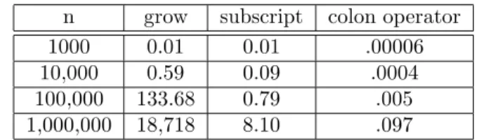
Table 2.1 shows the timing in seconds on a particular (old) machine of these three methods for a selection of values ofn. The relationships for varyingn are all roughly linear on a log-log scale, but the timings are drastically different.

You may wonder why growing objects is so slow. It is the computational equivalent of suburbanization. When a new size is required, there will not be

Table 2.1: Time in seconds of methods to create a sequence.

n grow subscript colon operator

1000 0.01 0.01 .00006

10,000 0.59 0.09 .0004

100,000 133.68 0.79 .005

(14)

CIRCLE 2. GROWING OBJECTS

enough room where the object is; so it needs to move to a more open space. Then that space will be too small, and it will need to move again. It takes a lot of time to move house. Just as in physical suburbanization, growing objects can spoil all of the available space. You end up with lots of small pieces of available memory, but no large pieces. This is called fragmenting memory.

A more common—and probably more dangerous—means of being a glutton is withrbind. For example:

my.df <- data.frame(a=character(0), b=numeric(0)) for(i in 1:n) _{

my.df <- rbind(my.df, data.frame(a=sample(letters, 1), b=runif(1)))

}

Probably the main reason this is more common is because it is more likely that each iteration will have a different number of observations. That is, the code is more likely to look like:

my.df <- data.frame(a=character(0), b=numeric(0)) for(i in 1:n) _{

this.N <- rpois(1, 10)

my.df <- rbind(my.df, data.frame(a=sample(letters, this.N, replace=TRUE), b=runif(this.N)))

}

Often a reasonable upper bound on the size of the final object is known. If so, then create the object with that size and then remove the extra values at the end. If the final size is a mystery, then you can still follow the same scheme, but allow for periodic growth of the object.

current.N <- 10 * n

my.df <- data.frame(a=character(current.N), b=numeric(current.N))

count <- 0 for(i in 1:n) _{

if(count + this.N > current.N) _{ old.df <- my.df

current.N <- round(1.5 * (current.N + this.N)) my.df <- data.frame(a=character(current.N),

b=numeric(current.N))

my.df[1:count,] <- old.df[1:count, ]

}

my.df[count + 1:this.N,] <- data.frame(a=sample(letters, this.N, replace=TRUE), b=runif(this.N))

count <- count + this.N

}

(15)

Figure 2.1: The giants by Sandro Botticelli.

Often there is a simpler approach to the whole problem—build a list of pieces and then scrunch them together in one go.

my.list <- vector(’list’, n) for(i in 1:n) {

my.list[[i]] <- data.frame(a=sample(letters, this.N replace=TRUE), b=runif(this.N))

}

my.df <- do.call(’rbind’, my.list)

There are ways of cleverly hiding that you are growing an object. Here is an example:

hit <- NA

for(i in 1:one.zillion) _{

if(runif(1) < 0.3) hit[i] <- TRUE

}

Each time the condition is true,hitis grown.

(16)

If you use too much memory, R will complain. The key issue is that R holds all the data in RAM. This is a limitation if you have huge datasets. The up-side is flexibility—in particular, R imposes no rules on what data are like.

You can get a message, all too familiar to some people, like:

Error: cannot allocate vector of size 79.8 Mb.

This is often misinterpreted along the lines of: “I have xxx gigabytes of memory, why can’t R even allocate 80 megabytes?” It is because R has already allocated a lot of memory successfully. The error message is about how much memory R was going after at the point where it failed.

The user who has seen this message logically asks, “What can I do about it?” There are some easy answers:

1. Don’t be a glutton by using bad programming constructs.

2. Get a bigger computer.

3. Reduce the problem size.

If you’ve obeyed the first answer and can’t follow the second or third, then your alternatives are harder. One is to restart the R session, but this is often ineffective.

Another of those hard alternatives is to explore where in your code the memory is growing. One method (on at least one platform) is to insert lines like:

cat(’point 1 mem’, memory.size(), memory.size(max=TRUE), ’_\n’)

throughout your code. This shows the memory that R currently has and the maximum amount R has had in the current session.

However, probably a more efficient and informative procedure would be to use Rprof with memory profiling. Rprof also profiles time use.

Another way of reducing memory use is to store your data in a database and only extract portions of the data into R as needed. While this takes some time to set up, it can become quite a natural way to work.

A “database” solution that only uses R is to save (as in thesavefunction) objects in individual files, then use the files one at a time. So your code using the objects might look something like:

for(i in 1:n) _{

objname <- paste(’obj.’, i, sep=’’) load(paste(objname, ’.rda’, sep=’’)) the obj <- get(objname)

rm(list=objname) # use the obj

(17)

Are tomorrow’s bigger computers going to solve the problem? For some people, yes—their data will stay the same size and computers will get big enough to hold it comfortably. For other people it will only get worse—more powerful computers means extraordinarily larger datasets. If you are likely to be in this latter group, you might want to get used to working with databases now.

If you have one of those giant computers, you may have the capacity to attempt to create something larger than R can handle. See:

?’Memory-limits’

(18)

Circle 3

Failing to Vectorize

We arrive at the third Circle, filled with cold, unending rain. Here stands Cerberus barking out of his three throats. Within the Circle were the blas-phemous wearing golden, dazzling cloaks that inside were all of lead—weighing them down for all of eternity. This is where Virgil said to me, “Remember your science—the more perfect a thing, the more its pain or pleasure.”

Here is some sample code:

lsum <- 0

for(i in 1:length(x)) {

lsum <- lsum + log(x[i])

}

No. No. No.

This is speaking R with a C accent—a strong accent. We can do the same thing much simpler:

lsum <- sum(log(x))

This is not only nicer for your carpal tunnel, it is computationally much faster. (As an added bonus it avoids the bug in the loop whenxhas length zero.)

The command above works because of vectorization. The log function is vectorized in the traditional sense—it does the same operation on a vector of values as it would do on each single value. That is, the command:

log(c(23, 67.1))

has the same result as the command:

c(log(23), log(67.1))

(19)

CIRCLE 3. FAILING TO VECTORIZE

x[1] + x[2] + ... + x[length(x)]

Theprodfunction is similar tosum, but does products rather than sums. Prod-ucts can often overflow or underflow (a suburb of Circle 1)—taking logs and doing sums is generally a more stable computation.

You often get vectorization for free. Take the example ofquadratic.formula in Circle 1 (page9). Since the arithmetic operators are vectorized, the result of this function is a vector if any or all of the inputs are. The only slight problem is that there are two answers per input, so the call to cbind is used to keep track of the pairs of answers.

In binary operations such as:

c(1,4) + 1:10

recycling automatically happens along with the vectorization.

Here is some code that combines both this Circle and Circle 2 (page12): ans <- NULL

for(i in 1:507980) _{

if(x[i] < 0) ans <- c(ans, y[i])

}

This can be done simply with:

ans <- y[x < 0]

A doubleforloop is often the result of a function that has been directly trans-lated from another language. Translations that are essentially verbatim are unlikely to be the best thing to do. Better is to rethink what is happening with R in mind. Using direct translations from another language may well leave you longing for that other language. Making good translations may well leave you marvelling at R’s strengths. (The catch is that you need to know the strengths in order to make the good translations.)

If you are translating code into R that has a doubleforloop, think.

If your function is not vectorized, then you can possibly use theVectorize function to make a vectorized version. But this is vectorization from an external point of view—it is not the same as writing inherently vectorized code. The Vectorizefunction performs a loop using the original function.

Some functions take a function as an argument and demand that the function be vectorized—these includeouterandintegrate.

There is another form of vectorization:

> max(2, 100, -4, 3, 230, 5)

[1] 230

> range(2, 100, -4, 3, 230, 5, c(4, -456, 9))

(20)

CIRCLE 3. FAILING TO VECTORIZE

Figure 3.1: The hypocrites by Sandro Botticelli.

This form of vectorization is to treat the collection of arguments as the vector. This is NOT a form of vectorization you should expect, it is essentially foreign to R—min,max,range,sumandprodare rare exceptions. In particular,meandoes not adhere to this form of vectorization, and unfortunately does not generate an error from trying it:

> mean(2, -100, -4, 3, -230, 5)

[1] 2

But you get the correct answer if you add three (particular) keystrokes:

> mean(c(2, -100, -4, 3, -230, 5))

[1] -54

One reason for vectorization is for computational speed. In a vector operation there is always a loop. If the loop is done in C code, then it will be much faster than if it is done in R code. In some cases, this can be very important. In other cases, it isn’t—a loop in R code now is as fast as the same loop in C on a computer from a few years ago.

Another reason to vectorize is for clarity. The command:

(21)

3.1. SUBSCRIPTING CIRCLE 3. FAILING TO VECTORIZE

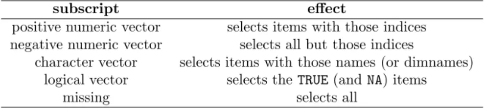
Table 3.1: Summary of subscripting with 8[8.

subscript effect

positive numeric vector selects items with those indices negative numeric vector selects all but those indices

character vector selects items with those names (or dimnames) logical vector selects theTRUE(andNA) items

missing selects all

clearly expresses the relation between the variables. This same clarity is present whether there is one item or a million. Transparent code is an important form of efficiency. Computer time is cheap, human time (and frustration) is expensive. This fact is enshrined in the maxim of Uwe Ligges.

Uwe0s MaximComputers are cheap, and thinking hurts.

A fairly common question from new users is: “How do I assign names to a group of similar objects?” Yes, you can do that, but you probably don’t want to—better is to vectorize your thinking. Put all of the similar objects into one list. Subsequent analysis and manipulation is then going to be much smoother.

3.1 Subscripting

Subscripting in R is extremely powerful, and is often a key part of effective vectorization. Table3.1 summarizes subscripting.

The dimensions of arrays and data frames are subscripted independently.

Arrays (including matrices) can be subscripted with a matrix of positive numbers. The subscripting matrix has as many columns as there are dimensions in the array—so two columns for a matrix. The result is a vector (not an array) containing the selected items.

Lists are subscripted just like (other) vectors. However, there are two forms of subscripting that are particular to lists: 8$8 and 8[[8. These are almost the same, the difference is that 8$8 expects a name rather than a character string.

> mylist <- list(aaa=1:5, bbb=letters)

> mylist$aaa

[1] 1 2 3 4 5 > mylist[[’aaa’]]

[1] 1 2 3 4 5

> subv <- ’aaa’; mylist[[subv]]

[1] 1 2 3 4 5

(22)

3.2. VECTORIZED IF CIRCLE 3. FAILING TO VECTORIZE

a single item is demanded. If you are using 8[[8 and you want more than one item, you are going to be disappointed.

We’ve already seen (in thelsumexample) that subscripting can be a symp-tom of not vectorizing.

As an example of how subscripting can be a vectorization tool, consider the following problem: We have a matrixamatand we want to produce a new matrix with half as many rows where each row of the new matrix is the product of two consecutive rows ofamat.

It is quite simple to create a loop to do this:

bmat <- matrix(NA, nrow(amat)/2, ncol(amat))

for(i in 1:nrow(bmat)) bmat[i,] <- amat[2*i-1,] * amat[2*i,]

Note that we have avoided Circle 2 (page12) by preallocatingbmat.

Later iterations do not depend on earlier ones, so there is hope that we can eliminate the loop. Subscripting is the key to the elimination:

> bmat2 <- amat[seq(1, nrow(amat), by=2),] *

+ amat[seq(2, nrow(amat), by=2),]

> all.equal(bmat, bmat2)

[1] TRUE

3.2 Vectorized if

Here is some code:

if(x < 1) y <- -1 else y <- 1

This looks perfectly logical. And if xhas length one, then it does as expected. However, ifxhas length greater than one, then a warning is issued (often ignored by the user), and the result is not what is most likely intended. Code that fulfills the common expectation is:

y <- ifelse(x < 1, -1, 1)

Another approach—assumingxis never exactly 1—is:

y <- sign(x - 1)

This provides a couple of lessons:

1. The condition inifis one of the few places in R where a vector (of length greater than 1) is not welcome (the 8:8 operator is another).

(23)

3.3. VEC IMPOSSIBLE CIRCLE 3. FAILING TO VECTORIZE

Recall that in Circle 2 (page12) we saw: hit <- NA

for(i in 1:one.zillion) _{

if(runif(1) < 0.3) hit[i] <- TRUE

}

One alternative to make this operation efficient is:

ifelse(runif(one.zillion) < 0.3, TRUE, NA)

If there is a mistake betweenifand ifelse, it is almost always trying to use ifwhen ifelse is appropriate. But ingenuity knows no bounds, so it is also possible to try to useifelsewhenifis appropriate. For example:

ifelse(x, character(0), ’’)

The result of ifelse is ALWAYS the length of its first (formal) argument. Assuming thatxis of length 1, the way to get the intended behavior is:

if(x) character(0) else ’’

Some more caution is warranted withifelse: the result gets not only its length from the first argument, but also its attributes. If you would like the answer to have attributes of the other two arguments, you need to do more work. In Circle8.2.7we’ll see a particular instance of this with factors.

3.3 Vectorization impossible

Some things are not possible to vectorize. For instance, if the present iteration depends on results from the previous iteration, then vectorization is usually not possible. (But some cases are covered byfilter,cumsum, etc.)

If you need to use a loop, then make it lean:

• Put as much outside of loops as possible. One example: if the same or a similar sequence is created in each iteration, then create the sequence first and reuse it. Creating a sequence is quite fast, but appreciable time can accumulate if it is done thousands or millions of times.

• Make the number of iterations as small as possible. If you have the choice of iterating over the elements of a factor or iterating over the levels of the factor, then iterating over the levels is going to be better (almost surely).

The following bit of code gets the sum of each column of a matrix (assuming the number of columns is positive):

sumxcol <- numeric(ncol(x))

(24)

3.3. VEC IMPOSSIBLE CIRCLE 3. FAILING TO VECTORIZE

A more common approach to this would be:

sumxcol <- apply(x, 2, sum)

Since this is a quite common operation, there is a special function for doing this that does not involve a loop in R code:

sumxcol <- colSums(x)

There are alsorowSums,colMeansandrowMeans. Another approach is:

sumxcol <- rep(1, nrow(x)) %*% x

(25)

Circle 4

Over-Vectorizing

We skirted past Plutus, the fierce wolf with a swollen face, down into the fourth Circle. Here we found the lustful.

It is a good thing to want to vectorize when there is no effective way to do so. It is a bad thing to attempt it anyway.

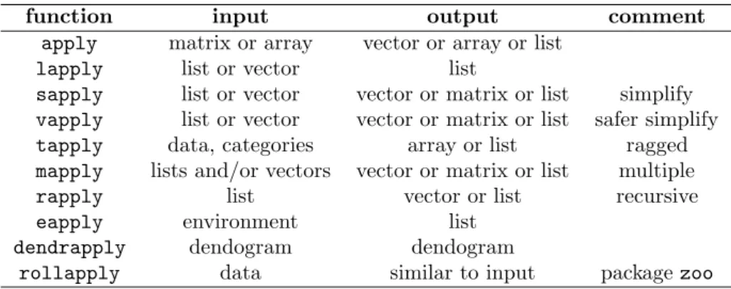
A common reflex is to use a function in the apply family. This is not vector-ization, it is loop-hiding. The applyfunction has a forloop in its definition. Thelapply function buries the loop, but execution times tend to be roughly equal to an explicitforloop. (Confusion over this is understandable, as there is a significant difference in execution speed with at least some versions of S+.) Table4.1summarizes the uses of the apply family of functions.

Base your decision of using an apply function on Uwe’s Maxim (page 20). The issue is of human time rather than silicon chip time. Human time can be wasted by taking longer to write the code, and (often much more importantly) by taking more time to understand subsequently what it does.

A command applying a complicated function is unlikely to pass the test.

Table 4.1: The apply family of functions.

function input output comment

apply matrix or array vector or array or list lapply list or vector list

sapply list or vector vector or matrix or list simplify vapply list or vector vector or matrix or list safer simplify tapply data, categories array or list ragged mapply lists and/or vectors vector or matrix or list multiple

rapply list vector or list recursive

eapply environment list

dendrapply dendogram dendogram

(26)

CIRCLE 4. OVER-VECTORIZING

Figure 4.1: The panderers and seducers and the flatterers by Sandro Botticelli.

Use an explicitforloop when each iteration is a non-trivial task. But a simple loop can be more clearly and compactly expressed using an apply function.

There is at least one exception to this rule. We will see in Circle8.1.56that if the result will be a list and some of the components can beNULL, then afor loop is trouble (big trouble) andlapplygives the expected answer.

Thetapplyfunction applies a function to each bit of a partition of the data. Alternatives to tapplyare by for data frames, and aggregatefor time series and data frames. If you have a substantial amount of data and speed is an issue, thendata.tablemay be a good solution.

Another approach to over-vectorizing is to use too much memory in the pro-cess. Theouterfunction is a wonderful mechanism to vectorize some problems. It is also subject to using a lot of memory in the process.

Suppose that we want to find all of the sets of three positive integers that sum to 6, where the order matters. (This is related to partitions in number theory.) We can useouterandwhich:

the.seq <- 1:4

which(outer(outer(the.seq, the.seq, ’+’), the.seq, ’+’) == 6, arr.ind=TRUE)

(27)

CIRCLE 4. OVER-VECTORIZING

problem. However, with larger problems this could easily eat all memory on a machine.

Suppose we have a data frame and we want to change the missing values to zero. Then we can do that in a perfectly vectorized manner:

x[is.na(x)] <- 0

But if x is large, then this may take a lot of memory. If—as is common—the number of rows is much larger than the number of columns, then a more memory efficient method is:

for(i in 1:ncol(x)) x[is.na(x[,i]), i] <- 0

Note that “large” is a relative term; it is usefully relative to the amount of available memory on your machine. Also note that memory efficiency can also be time efficiency if the inefficient approach causes swapping.

One more comment: if you really want to change NAs to 0, perhaps you should rethink what you are doing—the new data are fictional.

It is not unusual for there to be a tradeoff between space and time.

Beware the dangers of premature optimization of your code. Your first duty is to create clear, correct code. Only consider optimizing your code when:

• Your code is debugged and stable.

(28)

Circle 5

Not Writing Functions

We came upon the River Styx, more a swamp really. It took some convinc-ing, but Phlegyas eventually rowed us across in his boat. Here we found the treasoners.

5.1 Abstraction

A key reason that R is a good thing is because it is a language. The power of language is abstraction. The way to make abstractions in R is to write functions.

Suppose we want to repeat the integers 1 through 3 twice. That’s a simple command:

c(1:3, 1:3)

Now suppose we want these numbers repeated six times, or maybe sixty times. Writing a function that abstracts this operation begins to make sense. In fact, that abstraction has already been done for us:

rep(1:3, 6)

Therepfunction performs our desired task and a number of similar tasks. Let’s do a new task. We have two vectors; we want to produce a single vector consisting of the first vector repeated to the length of the second and then the second vector repeated to the length of the first. A vector being repeated to a shorter length means to just use the first part of the vector. This is quite easily abstracted into a function that usesrep:

repeat.xy <- function(x, y)

{

c(rep(x, length=length(y)), rep(y, length=length(x)))

}

(29)

5.1. ABSTRACTION CIRCLE 5. NOT WRITING FUNCTIONS

repeat.xy(1:4, 6:16)

The ease of writing a function like this means that it is quite natural to move gradually from just using R to programming in R.

In addition to abstraction, functions crystallize knowledge. Thatπis approx-imately 3.1415926535897932384626433832795028841971693993751058209749445 923078 is knowledge.

The function:

circle.area <- function(r) pi * r ^ 2

is both knowledge and abstraction—it gives you the (approximate) area for whatever circles you like.

This is not the place for a full discussion on the structure of the R language, but a comment on a detail of the two functions that we’ve just created is in order. The statement in the body of repeat.xyis surrounded by curly braces while the statement in the body of circle.areais not. The body of a function needs to be a single expression. Curly braces turn a number of expressions into a single (combined) expression. When there is only a single command in the body of a function, then the curly braces are optional. Curly braces are also useful with loops,switchandif.

Ideally each function performs a clearly specified task with easily understood inputs and return value. Very common novice behavior is to write one function that does everything. Almost always a better approach is to write a number of smaller functions, and then a function that does everything by using the smaller functions. Breaking the task into steps often has the benefit of making it more clear what really should be done. It is also much easier to debug when things go wrong.1 _{The small functions are much more likely to be of general use.}

A nice piece of abstraction in R functions is default values for arguments. For example, the na.rmargument to sd has a default value of FALSE. If that is okay in a particular instance, then you don’t have to specify na.rmin your call. If you want to remove missing values, then you should includena.rm=TRUE as an argument in your call. If you create your own copy of a function just to change the default value of an argument, then you’re probably not appreciating the abstraction that the function gives you.

Functions return a value. The return value of a function is almost always the reason for the function’s existence. The last item in a function definition is returned. Most functions merely rely on this mechanism, but the return function forces what to return.

The other thing that a function can do is to have one or more side effects. A side effect is some change to the system other than returning a value. The philosophy of R is to concentrate side effects into a few functions (such asprint, plotandrm) where it is clear that a side effect is to be expected.

(30)

Table 5.1: Simple objects.

object type examples

logical atomic TRUE FALSE NA

numeric atomic 0 2.2 pi NA Inf -Inf NaN

complex atomic 3.2+4.5i NA Inf NaN

character atomic ’hello world’ ’’ NA

list recursive list(1:3, b=’hello’, C=list(3, c(TRUE, NA)))

NULL NULL

function function(x, y) x + 2 * y

formula y ~ x

Table 5.2: Some not so simple objects.

object primary attributes comment

data frame list class row.names a generalized matrix matrix vector dim dimnames special case of array

array vector dim dimnames usually atomic, not always factor integer levels class tricky little devils

The things that R functions talk about are objects. R is rich in objects. Table5.1shows some important types of objects.

You’ll notice that each of the atomic types have a possible value NA, as in “Not Available” and called “missing value”. When some people first get to R, they spend a lot of time trying to get rid of NAs. People probably did the same sort of thing when zero was first invented. NA is a wonderful thing to have available to you. It is seldom pleasant when your data have missing values, but life is much better withNAthan without.

R was designed with the idea that nothing is important. Let’s try that again: “nothing” is important. Vectors can have length zero. This is another stupid thing that turns out to be incredibly useful—that is, not so stupid after all. We’re not so used to dealing with things that aren’t there, so sometimes there are problems—we’ll see examples in Circle 8, Circle8.1.15for instance.

A lot of the wealth of objects has to do with attributes. Many attributes change how the object is thought about (both by R and by the user). An attribute that is common to most objects isnames. The attribute that drives object orientation is class. Table 5.2 lists a few of the most important types of objects that depend on attributes. Formulas, that were listed in the simple table, have class"formula"and so might more properly be in the not-so-simple list.

A common novice problem is to think that a data frame is a matrix. They look the same. They are not that same. See, for instance, Circle8.2.37.

The word “vector” has a number of meanings in R:

(31)

usage.

2. an object with no attributes (except possiblynames). This is the definition implied byis.vectorandas.vector.

3. an object that can have an arbitrary length (includes lists).

Clearly definitions 1 and 3 are contradictory, but which meaning is implied should be clear from the context. When the discussion is of vectors as opposed to matrices, it is definition 2 that is implied.

The word “list” has a technical meaning in R—this is an object of arbitrary length that can have components of different types, including lists. Sometimes the word is used in a non-technical sense, as in “search list” or “argument list”.

Not all functions are created equal. They can be conveniently put into three types.

There are anonymous functions as in:

apply(x, 2, function(z) mean(z[z > 0]))

The function given as the third argument toapplyis so transient that we don’t even give it a name.

There are functions that are useful only for one particular project. These are your one-off functions.

Finally there are functions that are persistently valuable. Some of these could well be one-off functions that you have rewritten to be more abstract. You will most likely want a file or package containing your persistently useful functions.

In the example of an anonymous function we saw that a function can be an argument to another function. In R, functions are objects just as vectors or matrices are objects. You are allowed to think of functions as data.

A whole new level of abstraction is a function that returns a function. The empirical cumulative distribution function is an example:

> mycumfun <- ecdf(rnorm(10))

> mycumfun(0)

[1] 0.4

Once you write a function that returns a function, you will be forever immune to this Circle.

In Circle 2 (page12) we briefly metdo.call. Some people are quite confused by do.call. That is both unnecessary and unfortunate—it is actually quite simple and is very powerful. Normally a function is called by following the name of the function with an argument list:

(32)

Thedo.callfunction allows you to provide the arguments as an actual list:

do.call("sample", list(x=10, size=5))

Simple.

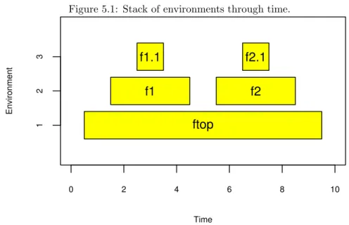
At times it is useful to have an image of what happens when you call a function. An environment is created by the function call, and an environment is created for each function that is called by that function. So there is a stack of environments that grows and shrinks as the computation proceeds.

Let’s define some functions:

ftop <- function(x)

{

# time 1 x1 <- f1(x) # time 5

ans.top <- f2(x1) # time 9

ans.top

}

f1 <- function(x)

{

# time 2

ans1 <- f1.1(x) # time 4

ans1

}

f2 <- function(x)

{

# time 6

ans2 <- f2.1(x) # time 8

ans2

}

And now let’s do a call:

# time 0 ftop(myx) # time 10

Figure 5.1 shows how the stack of environments for this call changes through time. Note that there is anxin the environments forftop,f1andf2. The x inftopis what we callmyx(or possibly a copy of it) as is thexinf1. But the xin f2is something different.

(33)

5.2. SIMPLICITY CIRCLE 5. NOT WRITING FUNCTIONS

Figure 5.1: Stack of environments through time.

Time

Environment

0 2 4 6 8 10

1

2

3

ftop

f1

f2

f1.1

f2.1

R is a language rich in objects. That is a part of its strength. Some of those objects are elements of the language itself—calls, expressions and so on. This allows a very powerful form of abstraction often called computing on the language. While messing with language elements seems extraordinarily esoteric to almost all new users, a lot of people moderate that view.

5.2 Simplicity

Make your functions as simple as possible. Simple has many advantages:

• Simple functions are likely to be human efficient: they will be easy to understand and to modify.

• Simple functions are likely to be computer efficient.

• Simple functions are less likely to be buggy, and bugs will be easier to fix.

• (Perhaps ironically) simple functions may be more general—thinking about the heart of the matter often broadens the application.

If your solution seems overly complex for the task, it probably is. There may be simple problems for which R does not have a simple solution, but they are rare.

Here are a few possibilities for simplifying:

(34)

5.3. CONSISTENCY CIRCLE 5. NOT WRITING FUNCTIONS

• Don’t use a data frame when a matrix will do.

• Don’t try to use an atomic vector when a list is needed.

• Don’t try to use a matrix when a data frame is needed.

Properly formatting your functions when you write them should be standard practice. Here “proper” includes indenting based on the logical structure, and putting spaces between operators. Circle8.1.30shows that there is a particularly good reason to put spaces around logical operators.

A semicolon can be used to mark the separation of two R commands that are placed on the same line. Some people like to put semicolons at the end of all lines. This highly annoys many seasoned R users. Such a reaction seems to be more visceral than logical, but there is some logic to it:

• The superfluous semicolons create some (imperceptible) inefficiency.

• The superfluous semicolons give the false impression that they are doing something.

One reason to seek simplicity is speed. TheRproffunction is a very convenient means of exploring which functions are using the most time in your function calls. (The nameRprofrefers to time profiling.)

5.3 Consistency

Consistency is good. Consistency reduces the work that your users need to expend. Consistency reduces bugs.

One form of consistency is the order and names of function arguments. Sur-prising your users is not a good idea—even if the universe of your users is of size 1.

A rather nice piece of consistency is always giving the correct answer. In order for that to happen the inputs need to be suitable. To insure that, the function needs to check inputs, and possibly intermediate results. The tools for this job includeif,stopandstopifnot.

Sometimes an occurrence is suspicious but not necessarily wrong. In this case a warning is appropriate. A warning produces a message but does not interrupt the computation.

There is a problem with warnings. No one reads them. People have to read error messages because no food pellet falls into the tray after they push the button. With a warning the machine merely beeps at them but they still get their food pellet. Never mind that it might be poison.

The appropriate reaction to a warning message is:

(35)

5.3. CONSISTENCY CIRCLE 5. NOT WRITING FUNCTIONS

2. Figure out why the warning is triggered.

3. Figure out the effect on the results of the computation (via deduction or experimentation).

4. Given the result of step 3, decide whether or not the results will be erro-neous.

You want there to be a minimal amount of warning messages in order to increase the probability that the messages that are there will be read. If you have a complex function where a large number of suspicious situations is possible, you might consider providing the ability to turn off some warning messages. Without such a system the user may be expecting a number of warning messages and hence miss messages that are unexpected and important.

ThesuppressWarningsfunction allows you to suppress warnings from spe-cific commands:

> log(c(3, -1))

[1] 1.098612 NaN Warning message:

In log(c(3, -1)) : NaNs produced > suppressWarnings(log(c(3, -1)))

[1] 1.098612 NaN

We want our functions to be correct. Not all functionsare correct. The results from specific calls can be put into 4 categories:

1. Correct.

2. An error occurs that is clearly identified.

3. An obscure error occurs.

4. An incorrect value is returned.

We like category 1. Category 2 is the right behavior if the inputs do not make sense, but not if the inputs are sensible. Category 3 is an unpleasant place for your users, and possibly for you if the users have access to you. Category 4 is by far the worst place to be—the user has no reason to believe that anything is wrong. Steer clear of category 4.

You should consistently write a help file for each of your persistent functions. If you have a hard time explaining the inputs and/or outputs of the function, then you should change the function. Writing a good help file is an excellent way of debugging the function. The promptfunction will produce a template for your help file.

(36)

Circle 6

Doing Global Assignments

Heretics imprisoned in flaming tombs inhabit Circle 6.

A global assignment can be performed with 8<<-8:

> x <- 1

> y <- 2

> fun

function () {

x <- 101 y <<- 102

}

> fun()

> x

[1] 1 > y

[1] 102

This is life beside a volcano.

If you think you need 8<<-8, think again. If on reflection you still think you need 8<<-8, think again. Only when your boss turns redwith anger over you not doing anything should you temporarily give in to the temptation. There have been proposals (no more than half-joking) to eliminate 8<<-8 from the language. That would not eliminate global assignments, merely force you to use theassignfunction to achieve them.

What’s so wrong about global assignments? Surprise.

Surprise in movies and novels is good. Surprise in computer code is bad.

(37)

CIRCLE 6. DOING GLOBAL ASSIGNMENTS

Figure 6.1: The sowers of discord by Sandro Botticelli.

A particular case where global assignment is useful (and not so egregious) is in memoization. This is when the results of computations are stored so that if the same computation is desired later, the value can merely be looked up rather than recomputed. The global variable is not so worrisome in this case because it is not of direct interest to the user. There remains the problem of name collisions—if you use the same variable name to remember values for two different functions, disaster follows.

In R we can perform memoization by using a locally global variable. (“locally global” is meant to be a bit humorous, but it succinctly describes what is going on.) In this example of computing Fibonacci numbers, we are using the 8<<-8 operator but using it safely:

fibonacci <- local(_{

memo <- c(1, 1, rep(NA, 100)) f <- function(x) _{

if(x == 0) return(0) if(x < 0) return(NA) if(x > length(memo))

stop("’x’ too big for implementation") if(!is.na(memo[x])) return(memo[x]) ans <- f(x-2) + f(x-1)

(38)

CIRCLE 6. DOING GLOBAL ASSIGNMENTS

ans

} })

So what is this mumbo jumbo saying? We have a function that is just imple-menting memoization in the naive way using the 8<<-8 operator. But we are hiding the memo object in the environment local to the function. And why is fibonaccia function? The return value of something in curly braces is what-ever is last. When defining a function we don’t generally name the object we are returning, but in this case we need to name the function because it is used recursively.

Now let’s use it:

> fibonacci(4)

[1] 3

> head(get(’memo’, envir=environment(fibonacci)))

[1] 1 1 2 3 NA NA

From computing the Fibonacci number for 4, the third and fourth elements of memohave been filled in. These values will not need to be computed again, a mere lookup suffices.

R always passes by value. It never passes by reference.

There are two types of people: those who understand the preceding para-graph and those who don’t.

If you don’t understand it, then R is right for you—it means that R is a safe place (notwithstanding the load of things in this document suggesting the contrary). Translated into humanspeak it essentially says that it is dreadfully hard to corrupt data in R. But ingenuity knows no bounds ...

(39)

Circle 7

Tripping on Object

Orientation

We came upon a sinner in the seventh Circle. He said, “Below my head is the place of those who took to simony before me—they are stuffed into the fissures of the stone.” Indeed, with flames held to the soles of their feet.

It turns out that versions of S (of which R is a dialect) are color-coded by the cover of books written about them. The books are: the brown book, the blue book, the white book and the green book.

7.1 S3 methods

S3 methods correspond to the white book.

The concept in R of attributes of an object allows an exceptionally rich set of data objects. S3 methods make the class attribute the driver of an object-oriented system. It is an optional system. Only if an object has aclass attribute do S3 methods really come into effect.

There are some functions that are generic. Examples includeprint,plot, summary. These functions look at the class attribute of their first argument. If that argument does have a class attribute, then the generic function looks for a methodof the generic function that matches the class of the argument. If such a match exists, then the method function is used. If there is no matching method or if the argument does not have a class, then the default method is used.

Let’s get specific. Thelm(linear model) function returns an object of class "lm". Among the methods for printare print.lmand print.default. The result of a call to lmis printed with print.lm. The result of 1:10is printed withprint.default.

(40)

7.1. S3 CIRCLE 7. TRIPPING ON OBJECT ORIENTATION

There is a cost to the free lunch. That printis generic means that what you see is not what you get (sometimes). In the printing of an object you may see a number that you want—an R-squared for example—but don’t know how to grab that number. If your mystery number is inobj, then there are a few ways to look for it:

print.default(obj) print(unclass(obj)) str(obj)

The first two print the object as if it had no class, the last prints an outline of the structure of the object. You can also do:

names(obj)

to see what components the object has—this can give you an overview of the object.

7.1.1 generic functions

Once upon a time a new user was appropriately inquisitive and wanted to know how the median function worked. So, logically, the new user types the function name to see it:

> median

function (x, na.rm = FALSE) UseMethod("median")

<environment: namespace:stats>

The new user then asks, “How can I find the code formedian?”

The answer is, “Youhave found the code for median.” medianis a generic function as evidenced by the appearance of UseMethod. What the new user meant to ask was, “How can I find the default method formedian?”

The most sure-fire way of getting the method is to usegetS3method:

getS3method(’median’, ’default’)

7.1.2 methods

The methods function lists the methods of a generic function. Alternatively given a class it returns the generic functions that have methods for the class. This statement needs a bit of qualification:

• It is listing what is currently attached in the session.

(41)

A list of all methods formedian(in the current session) is found with:

methods(median)

and methods for the"factor"class are found with:

methods(class=’factor’)

7.1.3 inheritance

Classes can inherit from other classes. For example:

> class(ordered(c(90, 90, 100, 110, 110)))

[1] "ordered" "factor"

Class"ordered"inherits from class"factor". Ordered factors are factors, but not all factors are ordered. If there is a method for"ordered" for a specific generic, then that method will be used when the argument is of class"ordered". However, if there is not a method for"ordered"but there is one for"factor", then the method for"factor"will be used.

Inheritance should be based on similarity of the structure of the objects, not similarity of the concepts for the objects. Matrices and data frames have similar concepts. Matrices are a specialization of data frames (all columns of the same type), so conceptually inheritance makes sense. However, matrices and data frames have completely different implementations, so inheritance makes no practical sense. The power of inheritance is the ability to (essentially) reuse code.

7.2 S4 methods

S4 methods correspond to the green book.

S3 methods are simple and powerful, and a bitad hoc. S4 methods remove thead hoc—they are more strict and more general. The S4 methods technology is a stiffer rope—when you hang yourself with it, it surely will not break. But that is basically the point of it—the programmer is restricted in order to make the results more dependable for the user. That’s the plan anyway, and it often works.

7.2.1 multiple dispatch

One feature of S4 methods that is missing from S3 methods (and many other object-oriented systems) is multiple dispatch. Suppose you have an object of class"foo"and an object of class"bar"and want to perform functionfunon these objects. The result of

(42)

Figure 7.1: The Simoniacs by Sandro Botticelli.

may or may not to be different from

fun(bar, foo)

If there are many classes or many arguments to the function that are sensitive to class, there can be big complications. S4 methods make this complicated situation relatively simple.

We saw thatUseMethodcreates an S3 generic function. S4 generic functions are created withstandardGeneric.

7.2.2 S4 structure

S4 is quite strict about what an object of a specific class looks like. In contrast S3 methods allow you to merely add aclassattribute to any object—as long as a method doesn’t run into anything untoward, there is no penalty. A key advantage in strictly regulating the structure of objects in a particular class is that those objects can be used in C code (via the .Callfunction) without a copious amount of checking.

(43)

7.3. NSPACES CIRCLE 7. TRIPPING ON OBJECT ORIENTATION

x@Data

that is an indication thatxis an S4 object.

By now you will have noticed that S4 methods are driven by the class attribute just as S3 methods are. This commonality perhaps makes the two systems appear more similar than they are. In S3 the decision of what method to use is made in real-time when the function is called. In S4 the decision is made when the code is loaded into the R session—there is a table that charts the relationships of all the classes. TheshowMethodsfunction is useful to see the layout.

S4 has inheritance, as does S3. But, again, there are subtle differences. For example, a concept in S4 that doesn’t resonate in S3 iscontains. If S4 class"B" has all of the slots that are in class"A", then class"B"contains class"A".

7.2.3 discussion

Will S4 ever totally supplant S3? Highly unlikely. One reason is backward compatibility—there is a whole lot of code that depends on S3 methods. Addi-tionally, S3 methods are convenient. It is very easy to create aplotorsummary method for a specific computation (a simulation, perhaps) that expedites anal-ysis.

So basically S3 and S4 serve different purposes. S4 is useful for large, industrial-strength projects. S3 is useful forad hoc projects.

If you are planning on writing S4 (or even S3) methods, then you can defi-nitely do worse than getting the bookSoftware for Data Analysis: Programming with Rby John Chambers. Don’t misunderstand: this book can be useful even if you are not using methods.

Two styles of object orientation are hardly enough. Luckily, there are the OOP,R.ooandprotopackages that provide three more.

7.3 Namespaces

Namespaces don’t really have much to do with object-orientation. To the casual user they are related in that both seem like an unwarranted complication. They are also related in the sense that that seeming complexity is actually simplicity in disguise.

Suppose that two packages have a function calledrecode. You want to use a particular one of these two. There is no guarantee that the one you want will always be first on the search list. That is the problem for which namespaces are the answer.

(44)

7.3. NSPACES CIRCLE 7. TRIPPING ON OBJECT ORIENTATION

namespace exports one or more objects so that they are visible, but may have some objects that are private.

The way to specify an object from a particular namespace is to use the 8::8 operator:

> stats::coef

function (object, ...) UseMethod("coef")

This operator fails if the name is not exported:

> stats::coef.default

Error: ’coef.default’ is not an exported object from ’namespace:stats’

There are ways to get the non-exported objects, but you have to promise not to use them except to inspect the objects. You can use 8:::8 or thegetAnywhere function:

> stats:::coef.default

function (object, ...) object$coefficients

<environment: namespace:stats> > getAnywhere(’coef.default’)

A single object matching ’coef.default’ was found It was found in the following places

registered S3 method for coef from namespace stats namespace:stats

with value

function (object, ...) object$coefficients

There can be problems if you want to modify a function that is in a namespace. FunctionsassignInNamespaceandunlockBindingcan be useful in this regard.

(45)

Circle 8

Believing It Does as

Intended

In this Circle we came across the fraudulent—each trapped in their own flame.

This Circle is wider and deeper than one might hope. Reasons for this include:

• Backwards compatibility. There is roughly a two-decade history of com-patibility to worry about. If you are a new user, you will think that rough spots should be smoothed out no matter what. You will think differ-ently if a new version of R breaks your code that has been working. The larger splinters have been sanded down, but this still leaves a number of annoyances to adjust to.

• R is used both interactively and programmatically. There is tension there. A few functions make special arrangements to make interactive use easier. These functions tend to cause trouble if used inside a function. They can also promote false expectations.

• R does a lot.

In this Circle we will meet a large number of ghosts, chimeras and devils. These can often be exorcised using thebrowserfunction. Put the command:

browser()

at strategic locations in your functions in order to see the state of play at those points. A close alternative is:

(46)

CIRCLE 8. BELIEVING IT DOES AS INTENDED

browserallows you to look at the objects in the function in which thebrowser call is placed. recoverallows you to look at those objects as well as the objects in the caller of that function and all other active functions.

Liberal use ofbrowser,recover,catandprintwhile you are writing func-tions allows your expectafunc-tions and R’s expectafunc-tions to converge.

A very handy way of doing this is withtrace. For example, if browsing at the end of themyFunfunction is convenient, then you can do:

trace(myFun, exit=quote(browser()))

You can customize the tracing with a command like:

trace(myFun, edit=TRUE)

If you run into an error, then debugging is the appropriate action. There are at least two approaches to debugging. The first approach is to look at the state of play at the point where the error occurs. Prepare for this by setting theerror option. The two most likely choices are:

options(error=recover)

or

options(error=dump.frames)

The difference is that with recoveryou are automatically thrown into debug mode, but withdump.framesyou start debugging by executing:

debugger()

In either case you are presented with a selection of the frames (environments) of active functions to inspect.

You can force R to treat warnings as errors with the command:

options(warn=2)

If you want to set the error option in your .First function, then you need a trick since not everything is in place at the time that.Firstis executed:

options(error=expression(recover()))

or

options(error=expression(dump.frames()))

The second idea for debugging is to step through a function as it executes. If you want to step through functionmyfun, then do:

debug(myfun)

and then execute a statement involvingmyfun. When you are done debugging, do:

undebug(myfun)

(47)

8.1. GHOSTS CIRCLE 8. BELIEVING IT DOES AS INTENDED

8.1 Ghosts

8.1.1 differences with S+

There are a number of differences between R and S+.

The differences are given in the R FAQ (http://cran.r-project.org/faqs.html). A few, but not all, are also mentioned here.

8.1.2 package functionality

Suppose you have seen a command that you want to try, such as

fortune(’dog’)

You try it and get the error message:

Error: could not find function "fortune"

You, of course, think that your installation of R is broken. I don’t have evidence that your installation is not broken, but more likely it is because your current R session does not include the package where thefortunefunction lives. You can try:

require(fortune)

Whereupon you get the message:

Error in library(package, ...) :

there is no package called ’fortune’

The problem is that you need to install the package onto your computer. As-suming you are connected to the internet, you can do this with the command:

install.packages(’fortune’)

After a bit of a preamble, you will get:

Warning message:

package ’fortune’ is not available

Now the problem is that we have the wrong name for the package. Capitalization as well as spelling is important. The successful incantation is:

install.packages(’fortunes’) require(fortunes)

fortune(’dog’)

Installing the package only needs to be done once, attaching the package with therequirefunction needs to be done in every R session where you want the functionality.

The command:

library()

(48)

Figure 8.1: The falsifiers: alchemists by Sandro Botticelli.

8.1.3 precedence

It is a sin to assume that code does what is intended. The following command clearly intends to produce a sequence from one to one less thann:

1:n-1

From the presence of the example here, you should infer that is not what you get.

Here is another way to make a similar mistake:

10^2:6

If you do:

-2.3 ^ 4.5

you will get a nice, pleasing number. If you do:

x <- -2.3 x ^ 4.5

(49)

as.complex(x) ^ 4.5

Pay attention to the precedence of operators. If you are at all unsure, then parentheses can force the command to do what you want.

You can see R’s precedence table by doing:

> ?Syntax

8.1.4 equality of missing values

The following can not possibly work to test for missing values inx:

x == NA

Why not?

Here’s a hint:

3 == c(3, 1, 3, NA)

Instead, do:

is.na(x)

8.1.5 testing NULL

Likewise there isis.nullfor testing if an object isNULL.

> xnull <- NULL

> xnull == NULL

logical(0) > xnotnull <- 42

> xnotnull == NULL

logical(0) > is.null(xnull)

[1] TRUE

However, it is often better to test if the length of the object is zero—NULLis not the only zero length object.

> is.null(numeric(0))

(50)

8.1.6 membership

Another common wish for the 8==8 operator is to indicate which elements of a vector are in some other vector. If you are lucky it will work, but generally does not. (Actually you will be unlucky if you are writing a function and it does work—you’ll miss the bug you just put in your function.)

> x1 <- 10:1

> x1 == c(4, 6)

[1] FALSE FALSE FALSE FALSE FALSE FALSE TRUE FALSE [9] FALSE FALSE

The command above fails to give the locations inx1that are equal to 4 and 6. Use 8%in%8 for situations like this:

> x1 %in% c(4, 6)

[1] FALSE FALSE FALSE FALSE TRUE FALSE TRUE FALSE [9] FALSE FALSE

8.1.7 multiple tests

If you want to do multiple tests, you don’t get to abbreviate. With thex1from just above:

> x1 == 4 | 6

[1] TRUE TRUE TRUE TRUE TRUE TRUE TRUE TRUE TRUE [10] TRUE

> x1 == (4 | 6)

[1] FALSE FALSE FALSE FALSE FALSE FALSE FALSE FALSE [9] FALSE TRUE

In a second we’ll discuss what is really happening in these two statements. It would be a good exercise for you to try to figure it out on your own.

But first, the way to actually do the intended operation is:

> x1 == 4 | x1 == 6

or (better for the more general case):

> x1 %in% c(4, 6)

Now, what are our bogus attempts doing?

The R Inferno - Free Computer, Programming, Mathematics, Technical Books, Lecture Notes and Tutorials

The R Inferno

Patrick Burns

30th April 2011

Contents

List of Figures

List of Tables

Preface

Circle 1

Falling into the Floating

Point Trap

Circle 2

Growing Objects

Circle 3

Failing to Vectorize

3.1

Subscripting

3.2

Vectorized if

3.3

Vectorization impossible

Circle 4

Over-Vectorizing

Circle 5

Not Writing Functions

5.1

Abstraction

ftop

f1

f2

f1.1

f2.1

5.2

Simplicity

5.3

Consistency

Circle 6

Doing Global Assignments

Circle 7

Tripping on Object

Orientation

7.1

S3 methods

7.1.1

generic functions

7.1.2

methods

7.1.3

inheritance

7.2

S4 methods

7.2.1

multiple dispatch

7.2.2

S4 structure

7.2.3

discussion

7.3

Namespaces

Circle 8

Believing It Does as

Intended

8.1

Ghosts

8.1.1

differences with S+

8.1.2

package functionality

8.1.3

precedence

8.1.4

equality of missing values

8.1.5

testing NULL

8.1.6

membership

8.1.7

multiple tests