Impedance Control of a Flexible Link Robot for
Constrained and Unconstrained Maneuvers
Using Sliding Mode Control (SMC) Method
G.R. Vossoughi
and A. Karimzadeh
1In this paper, the modeling and impedance-control of a one link exible robot is presented. The concept of impedance control of exible link robots is rather new and is being addressed for the rst time. The control algorithm is valid for both constrained and unconstrained maneuvers. First, equations of motion and the associated boundary conditions are derived using Hamilton's principle. A linear nite dimensional model is, then, generated in the Cartesian coordinates, using the assumed mode method and by introduction of a proper coordinate transformation. The target impedance is, then, introduced in the Cartesian coordinate system and a control law is designed to realize the proposed target impedance for a given frequency range, using the Sliding Mode Control Theory. A set of computer simulations are carried out to demonstrate the eectiveness of the proposed control law. Simulations are carried out with various contact stiness. As the results show, when the environmental surface stiness is smaller than, or comparable to, that of the link, the control system is able to achieve stable behavior and the link vibration diminishes rather rapidly. However, when the environmental stiness is much greater than that of the stiness of the link, although the robot achieves stable behavior during contact, the vibrations tend to increase.
INTRODUCTION
The closed-loop motion control systems fall, in gen-eral, into two dierent classes: unconstrained and constrained systems. In the rst case, the dynamic system (e.g., a manipulator) is driven in its workspace without contact with the environment. In the second case, the system is driven in its workspace in such a way that the environment continuously exerts a dynamic or kinematic constraint on the system's motion. A dynamic maneuver, such as leading a manipulator in a free environment towards a metal surface and, then, machine the surface, may consist of both types of maneuver.
The rejection of external forces is an important design specication when the dynamic system is
un-*. Corresponding Author, Department of Mechanical Engi-neering, Sharif University of Technology, Tehran, I.R. Iran.
1. Department of Mechanical Engineering, Civil Aviation Technology College, Tehran, I.R. Iran.
constrained. Once the system crosses the boundary of the unconstrained environment (i.e., the dynamic system interacts with the environment), the dynamics of the system will change and stability will no longer be guaranteed with the same controller. In constrained maneuvering, the interaction load must be accommo-dated rather than resisted. If one denes \compliancy" as a measure of the stability of a dynamic system to react to interaction forces and torques, one can state the objective as assuring compliant motion in the global Cartesian coordinate frame for dynamic systems that must maneuver in a constrained condition.
Three general approaches to the compliant motion control include: Impedance control, stiness control and hybrid position/force control. Hogan [1] rst presented the idea of impedance control. In this method, neither the position nor the forces are con-trolled. In impedance control, one rather dictates a pre-dened dynamic { often second-order and referred to as the target impedance - between the motion (position and orientation) and the interaction loads (forces and torques). An impedance control system reduces to a
position control system during unconstrained maneu-vers (because there are no interaction forces) and ac-commodates/controls contact forces during constrained conditions. Indeed, position control and force control are two extremes of impedance control. The former implies very high impedance, while the latter implies very low impedance.
Impedance control of rigid manipulators has been extensively addressed in the literature [1-6]. Many researchers have also considered the position, force and hybrid position/force control of exible manipula-tors [7-15]. However, the problem of impedance control of a exible manipulator has not yet been addressed in the literature. Impedance control provides a universal approach to the control of exible robots - in both constrained and unconstrained maneuvers. This also allows for controlling the compliance of exible robots/ structures beyond their natural compliance, making them more exible or rigid, as needed.
In this article, a novel impedance-control strat-egy is presented for a one-link exible manipulator using the Sliding Mode Control (SMC) theory. By including a term for the desired interaction force, the target impedance specication allows for force tracking during constrained maneuvers. Based on the SMC and eigenvalue assignment method, the dynamic system is forced in the sliding mode to achieve the desired impedance. Simulation results of the exible link, during the transition from an unconstrained to constrained condition (wall with specied stiness), are presented to demonstrate the eectiveness of the proposed impedance-control strategy.
MODELING
In this section, the modeling of a one degree of freedom exible robot is carried out for use under two conditions: Unconstrained and constrained state. In the rst case, it is assumed that the robot can move freely in its workspace without coming into contact with the environment. In the second case, it is assumed that the robot is in contact with an environment having a stiness,ke.
Modeling of anUnconstrained One-Link Flexible Robot
Let one consider a one-link exible robot with length,
l, mass per unit length,, and uniform exible rigidity,
EI, that is driven by a motor in the horizontal plane by a torque,. The beam is assumed to be clamped on the motor's shaft with moment of inertia,J, and having a tip point mass, M, at the end. Let be the angle of rotation of the rotor and oxy representing the moving coordinate system, xed to the rotor and rotating with angular velocity;(t) and angular acceleration, ,
Figure1. One-link exible robot during an unconstrained maneuver (with point massM).
about the inertial coordinate system, OXY. Referring to Figure 1, letW(x;t) denote the deformation of any point,x, andWe(t) =W(l;t) be the end deection of
the beam at any time,t. To write equations of motion, the following assumptions are made:
- The eects of nonlinear terms (W_)2 are small and
negligible;
- The joint angle (t) is assumed to be small (i.e., sin(), cos() = 1);
- The rotational eects and shear deformations are negligible and the link is modeled as an Euler-Bernoulli beam.
Given the above assumptions, for any given point along the beam, one may write:
y(x;t) =x w(x;t): (1) The total kinetic and potential energies and the virtual work done by the motor are, then, given by:
Ek= 12J_2+
2
l
Z 0
_
y(x;t)2dx
+ 12My_(l;t)2;
Ep=EI2
1 Z
0
y00(x;t)2dx;
W =: (2)
Using Hamilton's principal yields:
t
Z
t0
By separately calculating the variation of the parame-ter in Equation 3, one gets:
Ek =J_ _+ l
Z 0
( _yy_)dx+My_(l;t)y_(l;t);
Ep=EI l
Z 0
(y00y00)dx: (4)
Substituting Equation 4 into Equation 3 and using the integration by parts gives:
: J Zl 0
xy(x;t)dx Mly(l;t) +(t) = 0;
(5)
w: y(x;t) +EIy0000(x;t) = 0; (6)
y(l;t) : My(l;t) +EIy000(l;t) = 0: (7)
In obtaining the above equations, the following bound-ary conditions have been used:
w(0;t) =w0(0;t) =w00(l;t) = 0: (8)
By substituting Equation 6 into Equations 5 and 7, one gets:
J EIy 00(0;t) =(t); (9)
y(x;t) +EIy0000(x;t) = 0: (10)
The boundary conditions for Equation 10 are stated as:
y(0;t) =y00(l;t) = 0; y0(0;t) =(t);
M
y0000(l;t) +y000(l;t) = 0: (11)
By substituting Equation 1 into Equations 9 and 10, one obtains the equations of motion in the following forms:
j+EIw00(0;t) =(t); (12)
w(x;t) +EIw0000(x;t) =x; (13)
with the boundary conditions:
w(0;t) =w0(0;t) =w00(l;t) = 0; (14)
Mw0000(l;t) +w000(l;t) = 0: (15)
The above boundary Conditions are homogeneous, making the derivation of the nite dimensional modal model relatively straightforward using the assumed mode method.
Modelingof a Constrained One-LinkFlexible Robot
One now proceeds to model a one-link exible robot with its end-point in contact with an environment. As shown in Figure 2, it is assumed that the robot encounters a wall with a known stiness exerting a force,f(t), at the end-point of the robot.
The kinetic and potential energy of the link and the virtual work done by the motor may be written as:
Ek= 12J_2+
2
l
Z 0
_
y(x;t)2dx
+ 12My_(l;t)2;
Ep= EI2 l
Z 0
y00(x;t)2+f(t)y(l;t);
W =: (16)
Substituting Equation 16 into Equation 3 and integrat-ing by parts yields:
J Zl 0
xy(x;t)dx Mly(l;t)+(t) f(t)l=0; (17)
y(x;t) +EIy0000(x;t) = 0; (18)
EI(My(l;t) +y000(l;t)) +f(t) = 0: (19)
Equations 17 and 18 describe the equation of motion for the exible link. Equation 19 gives a boundary condition at x = l. The other three B.C's for Equation 18 are, as follows:
y(0;t) =y00(l;t) = 0; y0(0;t) =(t): (20)
Substituting Equation 18 into Equations 19 and 17, one
Figure 2. Constrained one-link exible robot in contact with environment (with known stinessKe).
obtains:
J EIy 00(0;t) =(t); (21)
y(x;t) +EIy0000(x;t) = 0; (22)
y(0;t) =y00(l;t) = 0; (23)
y0(0;t) =(t); (24)
EI
M
y0000(l;t) +y000(l;t)
= f(t): (25) Substituting Equation 1 into Equations 21 to 25 gives:
j+EIw00(0;t) =(t); (26)
w(x;t) +EIw0000(x;t) =x; (27)
w(0;t) =w0(0;t) =w00(l;t) = 0; (28)
EI
M
w0000(l;t) +w000(l;t)
=f(t): (29) Note that the boundary condition in Equation 29 is non-homogenous, calling for special attention. In the following section, a nite dimensional modal model will be derived for the robot in both unconstrained and constrained conditions, one that is suitable for the controller design applications.
CONSTRUCTION OFFINITE
DIMENSIONALMODEL
A nite dimensional model is constructed for both unconstrained and constrained cases. In order to con-struct a nite dimensional model, the eigen-function expansion method is used.
Unconstrained-Case
Substitutingw(x;t) =PN
i=1
'i(x)qi(t) into Equations 12
and 13 and multiplying every term by 'i(x), one
obtains:
qi(t) = !2
iqi(t) +bi ! 2
iq_i(t); (30)
J+EIXN
i=1
'00
i(0)qi(t) =(t): (31)
In which, 'i(x) represents the solution of the
Euler-Bernoulli beam (with the given boundary conditions), and !i and are the frequency of vibrations and
the small structural viscous damping of the beam's
material, respectively. Other parameters are dened as:
bi=< x;'i(x)>; (32)
< 'i;'j>= l
Z 0
'i'jdx+M 'i(l)'j(l);
< 'i;'j>= 0 ifi6=j: (33) Constrained-Case
Substitutingw(x;t) = PN
i=1
'i(x)qi(t) into Equations 26
and 27 and multiplying both sides by'i(x), results in:
qi(t)= !2
iqi(t)+bi ! 2
iq_i(t) ('i(l)=)f(t); (34)
J+EIXN
i=1
'00
i(0)qi(t) =(t); (35)
bi=< x;'i(x)>; (36)
where 'i(x) is the solution of the following equation
and boundary conditions:
'0000= (!2=EI)'; (37)
'(0) ='0(0) ='00(l) = 0; (38)
M'0000(l) +'000(l) = 0; (39)
and! is the frequency of vibrations.
MODELINGIN THECARTESIAN
COORDINATE SYSTEM
Since the target impedance is always dened in the Cartesian coordinate system, the dynamic model shall be expressed in the Cartesian coordinate system. One can use Equations 1 to construct a transformation between end point coordinate x(t) and the joint co-ordinate(t):
x(t) =l Xn
i=1
qi(t)'i(l): (40)
Dierentiating Equation 40 and using Equation 34, one gets:
x=ktu(t) +Xn
i=1
where:
kt=l Xn
i=1
bi'i(l); ki='i(l)!2
i;
ci=ki; a=Xn
i=1
'i(l)2=; (42)
and u(t) = (t) is considered as the control input. In Equation 34 and Equation 41, when the robot moves freely without any environmental contact, then,
f(t) = 0 and, as long as the endpoint is in contact with the environment, one hasf(t) = kex(t), whereke is
environmental stiness at the point of contact. Equations 34 and 41 can be written in the state space form, as follows:
_
X =AX+Bu+Bff(t); (43)
where:
A=
A11 A12
A21 A22
;
A22= 2 6 6 4
0 1 0 0 0
!2
1 !
2
1 0 0
0
0 0 0 1 0 0
0 0 !2
2 ! 2 2 0 0 3 7 7 5;
si= 'i ;(l)
A12=
0 0 0 0 0 0
k1 c1
kn cn
22n
; B2=
0 b1 0 b2
T 2n1;
A11= 0 0 0 1 22 ; Bf =
0 a 0 s1 0 s2
T
(2n+2)1;
B= B1 B2 ; A21= [0]2n2;
B1= 0 kt 21 : (44)
DESIGNOF ASLIDING MODE
CONTROLLER FOR ACHIEVING TARGET
IMPEDANCE
In this section, a control system is designed to achieve the desired target impedance. The controller en-ables one to control the behavior of the robot in the constrained as well as unconstrained condition. In the unconstrained case, in eect, the position will be controlled and in the constrained condition, a dynamic relationship between position error and contact force is controlled.
The target impedance is, usually, of the second order nature and is given by [4,5]:
Me+Ce_+Ke= f(t);
e=x(t) xd; (45)
where xd and f(t) are the desired end-point position
and contact force respectively. In a input multi-output case,M,CandKare positive denite matrices. In the next section, the role and the selection guidelines for each of the three parameters M, C and K will be discussed.
DESIGNOF THESLIDING SURFACE
In the previous section, the dynamics of the system were presented in state space form. Assuming that matrix B has full rank m (m is the number of inputs), there exists an orthogonal (2n+ 2)(2n+ 2)
transformation matrix,T, such that:
TB= 0 B2 ; (46)
where B2 is m
m and a nonsingular matrix. The
orthogonality restriction is onT, for reason of numeri-cal stability and to remove the problem of invertingT
when transforming back to the original system. A suit-able method for determiningT is theQU factorization, whereB is decomposed into the form:
B=Q
U
0
: (47)
WithQ nnand orthogonal, andU mm,
nonsin-gular and upper triannonsin-gular,T is, then, determined by rearranging the rows ofQT.
By writing Equation 43 in terms of the trans-formed state variable,y=TX, one has:
_
The transformed state, Y, and the state Equation 48 may be now partitioned as:
yT = [yT
1; y
T
2];
y1
2Rn m;
y2
2Rm; (49)
and the matricesTATT,TB andTBf are partitioned
accordingly, then, Equation 48 may be written in the form:
_
y1=A11y1+A12y2+Bf1f(t); (50)
_
y2=A21y1+A22y2+B2u+Bf2f(t); (51)
TATT =
A11 A12
A21 A22
: (52)
Now, if one denes the sliding surface as:
s=CX= 0: (53) The main goal will be the determination of elements of matrix C, so that the desired target impedance is obtained in the sliding mode.
The sliding surface, in terms of the transformed state,y, can be stated as:
s=(CTT)y=
C1 C2
y1 y2 T
=C1y1+C2y2=0:
(54) Condition 54, dening the sliding mode, may now be written as:
y2(t) = Fy1(t); (55)
where them(2n+ 2 m) matrix,F, is dened by:
F=C 1 2 C
1: (56)
This indicates that the evolution of y2 in the sliding
mode is related linearly to that ofy1. The ideal sliding
mode is, therefore, governed by the following equations: _
y1=A11y1+A12y2+Bf1f(t); (57)
y2(t) = Fy1(t); (58)
which is an (2n+ 2 m)th order system, in which
y2 plays the role of a state feedback controller.
Sub-stituting Equation 58 into Equation 57 results in the following closed loop dynamic:
_
y1= A11 A12F
y1+Bf1f(t); (59)
which indicates that the design of stable sliding mode dynamics (y1
! 0 as t ! 1) requires the
determi-nation of the gain matrix, F, such that A11 A12F
has (2n+2 m) left hand half-plane eigenvalues. This may be achieved using a conventional pole-placement method, i.e., one that minimizes an integral square cost function. Here, one can use the pole placement method to place the eigenvalues of Equation 59 in the desired locations. However, to achieve the target impedance Equation 45, one must choose the feedback gain, F, such that eigenvalues of Equations 59 and 45 are equal. In a multi-input case, one has to use the eigenstructure assignment method to match the dynamics of Equations 59 and 45. A problem which arises in a exible robot is that of the order of the dynamics in Equation 59 being much higher than that of Equation 45, depending upon the number of the assumed modes in the model. Hence, the eigenvalue assignment is nontrivial. This problem will be considered, in detail, in the next section.
It is noted that whichever scheme one chooses for the design, xing F does not uniquely determine C. This is due to the F =C 1
2 C
1 degrees of freedom in
the following relationship:
C2F =C1: (60)
A simple method of determiningC, is to let C2=Im
(identity matrix). This gives:
C=
F Imm
T: (61)
This approach has the merit of minimizing the amount of calculations and, hence, reducing the possibility of numerical error.
SLIDING MODECONTROLLER DESIGN
Now, one is ready to design a control law for achieving the desired impedance in Equation 45, i.e., bringing the systems state variables onto the sliding surface at a nite time and maintaining the state trajectory on the surface. Various methods are proposed for reaching the sliding surface. A simple reaching law, proposed by Slotine [16-18], is as follows:
_
s(t) = ksgn(s) s(t) Z t 0
s(t)dt; (62) where, and kare positive numbers. The sgn(s) is dened by:
sgn(s) =
8 > < > :
1 s >0 0 s= 0
1 s <0: (63) By dierentiating Equation 54 and substituting from Equations 62 and 43, one can obtain the following
control input:
u= (CB) 1
fCAX+CBff(t) +F(s)g; (64)
F(s) =ksgn(s) +s(t) +Z
s(t)dt; (65) in which det(CB) 6= 0 is the necessary condition
for controllability. The control law in Equation 64 guarantees that the system reaches the sliding surface at a nite time and stays on the sliding surface there-after. Once the sliding mode initiates, the dynamics in Equation 59 are realized and the desired impedance is achieved. The discontinuous function, sgn, in the control law Equation 64 causes high frequency chattering in the sliding mode, which is undesirable. To overcome this problem, the sgn(.) function is replaced with the piecewise continuous function, sat(.):
sat(s=) =
8 > < > :
1 s > ' s=' jsj< '
1 s < '; (66)
in which, is a positive number, known as the boundary layer. This parameter must be chosen as small as possible to eliminate the chattering.
SELECTIONOF THETARGET
IMPEDANCE
In the previous section, the desired impedance was dened as:
Me+Ce_+Ke= f(t); 0< ! < !0; (67)
in which (0;!0) is the frequency interval at which one
wants to realize the desired impedance. One usually selects the K matrix to limit the desired interaction forces and torques. The choices of inertia matrix (M) and damping matrix C assure the achievement of !0
and stability of the system.
A small !0 will also allow one to meet strong
sets of stability robustness specications at high fre-quencies. On the other hand, with a very small !0,
stability robustness to parameter uncertainties may not be satised. This is true because stability robustness to parameter uncertainties assign a lower bond on!0.
To achieve a wide !0, one should have a good model
of the system at high frequencies (and, consequently, a weak set of stability robustness specications at high frequencies).
Because of the conict between the desired !0
and stability robustness to high frequency un-modeled dynamics, it is a struggle to meet both sets of specica-tions for a given model of uncertainty. The frequency range of operation,!0, cannot be selected to be of an
arbitrary wide, if a good model of the system does not
exist at high frequencies, while a good model of the system at high frequencies makes it possible to retain the target dynamics for a wider range of frequencies (0;!0).
EIGENVALUES ASSIGNMENT OFTHE
VIBRATION MODES
One of the main issues in the impedance control of exible link robots is that the number of eigenvalues of the target impedance is much smaller than the number of modes of the system. To overcome this, one must place the eigenvalues associated with the vibration modes far from the origin, relative to the eigenvalues of the target impedance. This makes the dynamics of the target impedance dominant.
Letting !i and i(i = 1n) be the frequency
and damping coecient of the ith vibration mode, the eigenvalues are placed at !ii !j, where
is a positive number that must be properly selected. In selecting , the control system must preserve the stability robustness specication over the frequency range (0;!0). Proper selection ofrequires experience
and understanding of the system. must be large enough to guarantee that the performance specication will be met, but also, small enough to fulll the stability robustness specication. Because one needs to have a relatively large (because i's are very small), one
has to choose the frequency range, !0, as small as
possible.
BEHAVIOR OF IMPEDANCE CONTROL IN
UNCONSTRAINED ANDCONSTRAINED
CONDITIONS
If, for a robot manipulator, the impedance in Equa-tion 45 is realized over a specied frequency range (0;!0), depending upon the environment with which
the robot interacts, one can consider two modes for impedance control. These modes are position control and regulating force control.
Unconstrained Case
Before any contact (and in the absence of any contact forcef(t) :f(t) = 0), the arm is actually under position control. In this phase, the governing impedance equation is:
Me+Ce_+Ke= f(t) = 0; e=x xd:
Thus, if the target impedance in Equation 45 is stable (by proper selection of parametersM,CandK), then, the error e =x xd is guaranteed to approach zero,
Constrained Case
After contact (and in the presence of contact forcef(t)) the arm is actually under endpoint \force compensa-tion". In this phase, the governing impedance equation (assumingxe= 0) is:
Me+Ce_+Ke= f(t) = Ke(x)
)Me+Ce_+ (K+Ke)e
= Ke(xd); (68)
wheree=x xd andKe= environmental stiness:
Steady state position error:
e= (KK+eKe)(xd)
x!
K K+Ke
xd; (69)
Steady state contact force:
f = Kex= KKK+Keexd;
f =K+KKefd: (70)
If one assumes the desired contact force is mod-ulated by the desired position, xd, as in fd =ke(xd),
then, one gets:
Steady state contact forcef= Ke:x=K+KKefd:
(71) Thus, under contact conditions, one can get controlled regulation of the contact forces by proper selection of the impedance parameter, K, or by location of the eigenvalues of the target impedance in Equation 45. Accurate control of the contact force requires the use of force error in the impedance control law and will not be pursued here.
COMPUTERSIMULATIONRESULTS
The simulations are carried out to demonstrate the eectiveness of the proposed impedance control law. The simulation is done for two cases: (a) A wall stiness, Ke = 100 (N/m) and (b) A wall stiness,
Ke= 1000 (N/m). Other assumed parameters are:
l= 0:9 (m); E= 2:06e11; I = 1:41e 11 (m4); = 0:405 (kg/m);
= 1:2e 4 (N.s/m); M= 0:66 (kg); J = 0:2; a= 1000; b= 500; k= 0:2;
xd= 0:08 + 0:05t (m) (for unconstrained case);
xd= 0:02 (for constrained case):
The equivalent stiness and mass at the end of the beam can be given by:
Keq= 3EIl3 >>12 [N/m];
Meq =l3 = 0:12 [kg]:
Impedance parameters for two cases are given as: for unconstrained phase:
M=0:06; C=2:1; K=16; !0=15(rad/s); =50;
for constrained phase:
M=0:06; C=1:8; K=12:5; !0=15(rad/s); =50;
contact time:
t= 1:6[sec]:
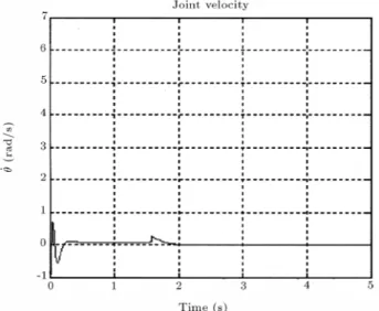
The simulation has been carried out using two modes for the controller design and using four modes for the model simulation. For each case, the rst mode q1(t), second mode, q2(t), end point position,
y(t), joint angle, (t), angular velocity, _(t), and contact force, f(t), are plotted. Figures 3 to 8 show the results for Case (a). As the results show, the link has a stable behavior before and during contact with the environment. Moreover, the vibration modes
Figure4. Transient response of _ for Case (a).
Figure5. Transient response of vibration Mode I for Case (a).
Figure6. Transient response of vibration Mode II for Case (a).
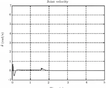
have also been shown to die out after contact. As discussed previously, before the contact (t < 1:6), the impedance controller acts as a simple position controller and, during the contact (t > 1:6), as a regulating force controller. As shown in Figures 7 and 8, there are steady state errors in the contact force and endpoint position, according to Equations 69 and 70. Figures 9 to 14 represent the results for Case (b). In this case, the stiness of the surface is much greater than that of the link. In this case, also, the link vibrations are damped out before and during the contact. In this case, separation did not occur, but, if the stiness of the environment increases, separation may also occur during the contact. As shown in Figures 13 and 14, steady state position and contact force errors in this case are larger than that of Case (a). This increase in the steady state errors resulting from higher environmental stiness is also predicted from
Figure 7. Transient response ofy(t) for Case (a).
Figure9. Transient response offor Case (b).
Figure10. Transient response of _for Case (b).
Figure11. Transient response of vibration Mode I for Case (b).
Figure12. Transient response of vibration Mode II in Case (b).
Figure13. Transient response ofy(t) for Case (b).
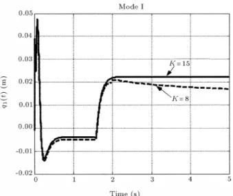
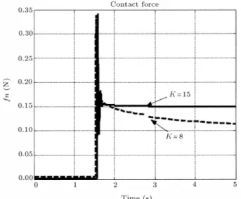
Equations 69 and 70. One should also note that, as the eigenvalues for target impedance are moved further to the left (in the left half plane), the eective endpoint stiness of the robot increases to values much larger than the inherent endpoint exibility and instability during contact becomes inevitable. Simulation with eigenvalues, < 20, leads to unstable behavior during contact (results not shown here). A simulation was also carried out with two sets of eigenvalues that correspond to the value of K = 8 N/m and K = 15 N/m (dierent from the inherent endpoint stiness
Keq 12 N/m), in order to show the eects of
parameter K on the impedance controller. These results are shown in Figures 15 to 20 and are labeled as Case (c).
Based on the above results, one can conclude that the proposed impedance control strategy has enabled one to control the behavior of the exible link robot in
Figure15. Transient response of for Case (c).
Figure16. Transient response of _ for Case (c).
Figure 17. Transient response of Mode I for Case (c).
Figure 18. Transient response of Mode II for Case (c).
Figure20. Transient response offn(t) for Case (c).
both constrained and unconstrained conditions, a ca-pability that would, otherwise, require two controllers, each with a dierent control structure.
CONCLUDING REMARKS
In this paper, the modeling and impedance control of a exible link manipulator, using a sliding mode control technique, have been considered. The pro-posed controller works well in both unconstrained and constrained conditions. One can control the behavior of the manipulator, in both conditions, using a single controller with a single structure (by only tuning the impedance parameters). The use of the sliding mode control theory provides a suitable domain for future research into issues such as robustness and the eects of various nonlinear eects, actuator dynamics and other uncertainties and external disturbances. These studies should be complemented by experimental results to further validate the proposed control method.
NOMENCLATURE
ke stiness of environment
L length of robot
mass per unit length
EI exural rigidity of link
M tip mass
joint angle
w(x;t) deection of any pointx at timet we(t) =w(l;t) end point deection of link
Ek kinetic energy
Ep potential energy
W virtual work done of motor
J moment inertia of rotor
f(t) normal contact force
!i(i= 1:::n) natural frequency of link
'i(x) mode shape of link
small structural damping of link
(t) torque developed by motor
x(t) end point position
xd(t) desired motion trajectory
M desired mass matrix
K desired stiness matrix
B desired damping matrix
u(t) control input
T transformation matrix
REFERENCES
1. Hogan, N. \Impedance control: An approach to manipulation: Part I, Part II, Part III", ASME J. Dynamic Syst. Measurement. Contr.,107(1), pp 1-24 (1987).
2. Kelly, R. and Carelli, R. et al. \Adaptive impedance control of robot manipulators", Int. J. Robotics and Automation,4(3), pp 134-141 (1989).
3. Kosuge, K. and Yokoyama, T. \Mechanical impedance control of robot arm by virtual internal model fol-lowing controller", Proc. IFAC 10th Triennial World Congress, Munich, Germany,4, pp 239-244 (1987). 4. Kazerooni, H. and Sheridan, T.B. et al. \Robust
compliant motion for manipulators, Part I: The funda-mental concept of compliant motion; Part II: Design method",IEEE. J. Robotics and Automation,2(2), pp 83-105 (1985).
5. Chan, S.P. and Gao, W.B. \Robust impedance control of robot manipulators", Int. J. Robotic and Automa-tion,6(4), pp 220-227 (1991).
6. Purboghart, F. \Virtual adaptive compliant control for robots",Int. J. Robotics and Automation,4(3), pp 148-157 (1988).
7. Raibert, M.H. and Craig, J.J. \Hybrid position/force control of manipulators", Trans. ASME J. Dyn. Sys. Meas. Control.,03(2), pp 126-133 (1981).
8. Khatib, O. \A unied approach to motion and force control of robot manipulators: The operational space formulation",IEEE Trans. Robotics Automation, RA-3(1), pp 43-53 (1987).
9. Oshikawa, T. \Dynamic hybrid position/force control of robot manipulators-description of hand constraints and calculation of joint driving force", IEEE Trans. Robotic Automation,RA-3(5), pp 386-392 (1987). 10. McClamroch, N.H. and Wang, D. \Feedback
stabiliza-tion and tracking of constrained robots",IEEE Trans Automatic Control,Ac-33(5), pp 419-426 (1988). 11. Fukada, T. \Flexibility control of elastic robotic arms",
12. Chiou, C. and Shahinpoor, M. \Dynamic stability analysis of two-link force-controlled exible manipu-lator",ASME J. Dyn. Sys. Meas. Control,112(6), pp 661-666 (1990).
13. Matsuno, F. and Sakawa, Y. et al. \Quasi-static hybrid position/force control of a exible manipulator",Proc. IEEE Int. Conf on Robotics and Automation, Sacra-mento, USA, pp 2838-2842 (1991).
14. Matsuno, F. and Asano, T. et al. \Quasi-static hybrid position/force control of two-degree-of-freedom exible manipulators", Proc. IEEE/RSJ Int. Workshop on Intelligent Robots and Systems'91 (IRSO'91), Osaka, Japan, pp 984-989 (1991).
15. Matsuno, F. and Yamamoto, K. \Dynamic hybrid po-sition/force control of a two degree-of freedom exible manipulator", Journal of Robotic Systems, 11(5), pp 355-366 (1994).
16. Slotine, J.J. and Li, W., Applied Nonlinear Control, Prentice-Hall (1990).
17. Li, D. and Slotine, J.J. \ On sliding control for multi-input multi-output nonlinear system",Proc. American Control Conf., pp 874-79 (1987).
18. Slotine, J.J. \Sliding controller design for nonlinear systems",Int. J. Control,40(2), pp 101-109 (1994).