Control of Under Actuated System with Input Constraints

Control of Under Actuated System with Input Constraints

Atif Alia)_{*, Muwahida Liaquat* and Mohammad Bilal Malik*}

1. Department of Electrical Engineering, College of Electrical and Mechanical Engineering, National University

of Sciences and Technology (NUST), Islamabad, Pakistan

* Corresponding Author: E-mail: [email protected]

Abstract

A pulse width modulation (PWM) approach based on the discrete equivalent model of an under actuated spinning body is proposed. The presented work is a sequel to the earlier work done by the authors for the orientation control of the drill machine. The constraint is an actuating signal of fixed amplitude with adjustable pulse width. A novel approach based on error minimization is developed. The optimized values of pulse width and phase of the control input are estimated to generate the actuating signal. The problems of local minima and non-causality were also addressed through proposed technique. The simulations are included to compare proposed techniques with the earlier developed techniques for similar systems. The performance is also shown under both nominal and parameter variations.

Key Words

: Under Actuated Control; Optimization; PWM; Global Minima

1. Introduction

Control of under actuated systems has attracted lot of attention from the researchers mainly because they are economically efficient. The applications of under actuated mechanical designs have shown significant improvement in the robust operating performance [1-4]. This also finds application in spin stabilized flying bodies, under actuated ships and satellite control schemes. The control of such under actuated systems has its limitations and can be classified as a challenging problem in the field of controls and dynamics. To drive such systems generally two types of actuators are utilized namely Servo and On-Off type [5,6] and the references therein. Amongst the two types, the control signal generated by servo actuators is more accurate and smooth on the other hand, on-off type is preferred due to its simpler structure such as gas-jet thrusters for satellites and solenoid valves for high-power hydraulic excavators. The consequent design of control systems for such actuators involves nonlinear analysis and design. Various techniques such as the Principle of Equivalent Areas (PEA) for PWM [7-12] are used to design the linear control systems having on-off actuation mechanism.

__________________________________

Note: This work was part of Ph.D. research work of Atif Ali and was fully supported by the National University of Sciences and Technology (NUST), Pakistan.

The orientation control of a special drill machine specifically designed for drilling soft materials was presented in [13,14]. This special drill machine [13] is a typical example of an under actuated spinning system. The magnitude and phase of the actuation pulse are controlled by a discrete time controller. The underlying model of the controller is the discrete-time equivalent model of the plant. The plant is actuated for a short duration i.e., during a complete revolution of the bit and is unactuated otherwise. This leads to an under actuated control problem. The solution provided by [13] is effective in controlling the orientation, but has a major practical limitation. The pulse width of control input is fixed while its magnitude is proportional to the amount of control force required and is unlimited. In physical system such unlimited amplitude leads to saturation. On the other hand, limiting the maximum amplitude of the control signal restricts the overall movement and leads to stability issues.

This paper is presented as a sequel of [13]& [15] with the focus on improving controller design. The limitation of unlimited amplitude can be overcome by assuming the actuation pulse of fixed amplitude and variable duration. This led to designing a more complex algorithm where the control input leads to inconvenient closed form time variant solution. Adjusting the pulse width and delay of such control input can be carried out through a PEA based

technique [15]. The main advantage of PEA is that it is practically implementable, but is based on approximation. Thus, for high modulation frequency, the averaging response becomes closer to the given control signal but at the same time higher model formulas are more difficult to convert using the PEA concept [8]. The minimum pulse width which cannot be ignored is also a major limitation for developing exact PEA signal. Therefore a novel technique is required to design the controller for such systems. It is a real challenge as the orthodox control theory is not applicable here. An output feedback optimization algorithm based on the minimization of the error signal is proposed. The resultant actuating signal is generated based on the optimized values of pulse width and delay. It is shown via simulations that the presented scheme provided a smooth control for precise movement and overcome the limitations on the control effort. The cost function, however, appears to be ill behaved, resulting in multiple local minima. The elimination of local minima and the estimation of unique global minima is carried out through reference phase algorithm and multiple

initial point algorithm (MIP) [16]. Global

minimization plays an effective role in many real problems such as science, engineering and economy [17]. The causality is also assured by employing a sliding adjustment technique.

Fig. 1. Under Actuated Drill Machine [13]

The remainder of the paper is organized as follows: Section 2 describes the model of the under actuated drill machine. The Error minimization control algorithm is presented in section 3 followed by the conclusion and references.

2. The Under Actuated Spinning Body

The plant is a small drill machine shown in the Fig.1. It spins about Z-axis, while up & down and right & left movements are about X-axis and Y-axis respectively. Due to the mounting limitations and its miniature size only a single pair of magnets is used. The required torque for orientation control of drill bit is produced through interaction of magnetic field of electromagnetic poles and rotor’s permanent magnet. The electromagnetic poles are excited for a short duration at specific roll phase resulting in one actuator, thus converting the fully actuated drill machine into an under actuated system. The construction of drill machine is explained in detail [13].

2.1 System Model

The frames of reference attached to the rotor and stator are X Y Z and X Y Z   respectively as shown in Fig. 2. The magnetic field and the torque

produced by rotor magnet are along the rotor’s Y and

X axis respectively. As the rotor is spinning,

therefore, when



_zt0o, the direction of the toque is along stator’sXaxis and when



_zt90o, the direction of the toque is along stator’s Y axis. The input torque with respect to the inertial frame is

ˆ

ˆ ˆ

i

x x y y z z d

H dt

H J



i J



j J



k



   (1)

Where, H is the angular momentum, ( ,J J J_{x y}, )_z are moments of inertia and

( ,

  

x y

,

z

)

are the angular

velocities along X Y Z axis respectively. The angular positions along X Y  axis are(

 

_x , _y) B is magnetic field due to stator winding and b is coefficient of friction.

A spinning drill bit with a high angular rate



_z

about Zaxis is in fact a two degrees of freedom gyroscope, therefore following model of gyroscope [18] is used:-

(2)

To represent (2) in state space form,

t

z y

x y

x











as x₁,x₂,x₃,x₄,u₁ and u₂ respectively. It is

assumed that



_zis constant which is quite typical in

spinning systems. The angular positions are obtained by integrating angular velocities. The corresponding linear time invariant state space equations are:

 

0 0 1 0

 

0 0 0 1

( ) cos

sin z

z

y t x t

u t t

t









 

  

 

 

  

 

(3)

Fig. 2 Direction of Actuation

2.2 Actuation Constraints

In the control scheme presented in [13], the drill machine is actuated by rectangular pulses of fixed

duration Ld and variable amplitude as shown in

Fig.3. The center of the actuation pulse is the point where the magnetic field of the rotor and the precession axis are precisely aligned. In each actuation cycle, the input pulse is applied after a time

delay  and the system remains unactuated for the

rest of cycle i.e., T–Ld The requirement of pulse width having unlimited amplitude is restricted to

maximum amplitude Umax. This limitation was

overcome by assuming the actuation pulse having fixed amplitude with variable duration. The actuation

cycle of period _{T applied for a complete revolution is}

constant and is shown in the Fig. 4. The phase of actuation  represents the shift of the center of the rectangular pulse from the start of the revolution. The

amplitude of the pulse is fixed and PWvaries

according to the requirement of the control signal

magnitude. ThereforePWand  are to be estimated

subject to the following constraints:-

 





1 2

2 1

0 where

2

t PW t

T

T t t

u t 



 



   _  



 _

(4)

Fig. 3 Single Actuation Cycle Amplitude Modulation [13]

Fig. 4 Single Actuation Cycle under Constraints(4)

3. Error Minimized Control (EMC)

PEA based scheme [15] and Amplitude Modulation approach [13] have their respective limitations. A novel algorithm is presented which is based on the optimization of the error signal. The complexity level is also increased by posing it as an output feedback control as opposed to the state feedback control [13].The discrete-time equivalent model is given by (5) (same as A.5). The detailed derivation is presented in appendix “A”.

T

(K+1)T

max U

KT

time t Ld



Y, X’

X

Y’

N

S

ωzt=900

X, X’ N

S

Y,Y ’

Z,Z’

ωzt=00

N

S

T

KT

time t

PW

α

∆

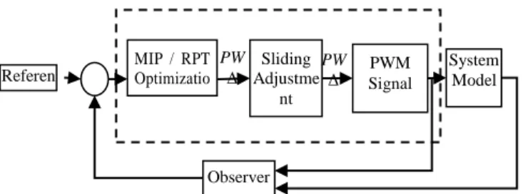
Fig. 5 Error Optimized Control Scheme









 

(K 1)

 

2 2 1 PW KT PW KT

AT AT A

x K T e x KT e e  Bu  d

       

_

(3) Although the integral in (5) is solvable but the closed form becomes inconveniently lengthy to handle. The control techniques presented in [13] and [15] are not applicable for systems that are not convenient to express in closed form. Due to this limitation we resort to use non-conventional method derived from optimal control and Model predictive control theory.

3.1 Controller

The pulse width PW and the position Δ are the only available parameters whose values can be controlled under constraints (4).The control signal (Fig. 4) is generated by searching optimized values of

PW and Δ based on the minimization of error. The Fig. 5 presents the proposed scheme. The error is the difference between the reference signal and the

observer feedback (6). The cost functionJ u( )is

given by (7)

(4)





2 2 2 2

1 2 3 4

( )

J u e e  e e (5)

The variable  is the weighting function.

Minimization of (7) based on the constraints (4) is a non-linear least square problem [19]. This can be

solved via interior-reflective Newton method [20]. The algorithm is a subspace trust-region method and

finds optimized values of PW and Δ

 

 

 









2 _{2 2 2 2}

1 2 3 4

2

, ,

min min

Pw J u  Pw e e  e e (6) Trust region methods mainly depend on the initial guess, therefore only for 1st_{iteration, some}

reasonable values of PW and ∆ were selected and for

subsequent iterations their previous values were taken as initial guess, as explained below :-

1 0 1 0 2 0 0 0 i i i i T i i PW i PW PW i    _   _{ }        _  (7)

For the proposed optimization algorithm, two problems were encountered. One is the problem of local minima. This problem can be effectively

neutralized through two different algorithms

discussed in detail in section 3.4. The other problem is that the actuation may become non-causal. This non-causality was denied through phase adjustment technique given in section 3.5.

3.2 Observer Design

0 0.5 1

-0.5 0 0.5 1 1.5 P o s it io n X -a x is Time

0 0.5 1

-2 -1 0 1 P o s it io n Y -a x is Time

0 0.5 1

-1 -0.5 0 0.5 E rr o r Time

0 0.5 1

0 0.2 0.4 0.6 0.8 J Time Cost Function

Obs e rve r Output R e fe re nce

Obs e rve r Output R e fe re nce

Along X-a xis Along Y-a xis

Fig. 6 EMC Based Control

The observer is designed via the standard pole placement technique [21] for EMC. The observer

gain

L

 



531



531



414



414



is designed for

such eigenvalues that the error (10) asymptotically converges to zero.

(8)

Error Minimized Control

(EMC)

P W

Δ

PW

Δ AdjustmeSliding nt PWM Signal System Model Observer MIP / RPT Optimizatio n Referen ce PW Δ

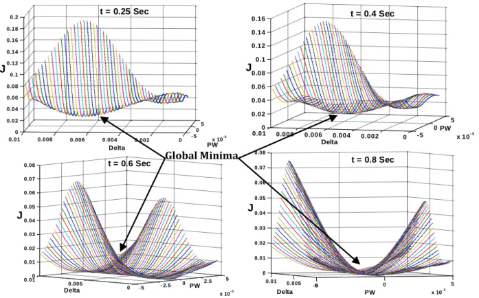
3.3 Local Minima Issues

The performance of the proposed EMC based control for the position control of X and Y axis is shown in Fig. 6. The system shows poor tracking response for the time interval 0.1sec to 0.5 sec (Fig. 6). This is due to the existence of at least two minima in addition to global minima. Hence, the optimizer cannot differentiate between local and global minima and consequently the cost function could not be minimized. This problem was investigated through exhaustive search for global minima at different time intervals (Fig. 7). The values for the optimized cost

function at 0.25 sec are (J(u), PW, 

are( ( )J u PW, , ) (90.044,0.0012, 0.0013) but this is a local minimum. The global minimum exists at( ( ),J u PW, ) (0.01, 0.0032, 0.0065). Similarly the same phenomenon of local minima is also observed at 0.4 sec. However, the situation is improved at 0.55 sec and 0.8 sec where the optimizer was able to converge to global minima effectively (because of the absence the local minima). In order to avoid local minima, two approaches in following sub-sections

were used. Both the methods were able to avoid local minima and show satisfactory results.

Reference Phase Algorithm (RPA)

For each iteration, the initial guess forand PW

is fed to the search algorithm. This initial guess foris calculated from the phase of the reference signal (11).The last value of PW is taken as initial guess for the next iteration.

1

0 1

0 2

tan 0

2

0 0 i

y x

i i

T

i r T

i r

PW i

PW

PW i

 



 _



   _{ }

 _{  }

 _{ }



 

  _



(9)

Multiple Initial Point (MIP) Algorithm

This algorithm is a comprehensive search technique for global minimization. It is initiated through multiple equi-spaced n data sets. The values of and PW are selected based on the lowest value

of the cost functionJ . Mathematically, the algorithm

is explained in (12),

-5 0

5

x 10-3

0 0.002 0.004 0.006 0.008

0.010

0.02 0.04 0.06 0.08 0.1 0.12 0.14 0.16

PW

t = 0.4 Sec

Delta

J

- 5 - 2. 5 0

2.5 5 x 10-3 0

0.005 0.010

0.01 0.02 0.03 0.04 0.05 0.06 0.07 0.08

PW

t = 0.6 Sec

Delta

J

- 5 0 5

x 10-3 0

0.005 0.01 0 0.01 0.02 0.03 0.04 0.05 0.06 0.07 0.08

t = 0.8 Sec

PW Delta

J

- 5 0

5 x 10-3 0

0.002 0.004 0.006 0.008 0.01

0 0.02 0.04 0.06 0.08 0.1 0.12 0.14 0.16 0.18 0.2

PW Delta

t = 0.25 Sec

J

Global Minima

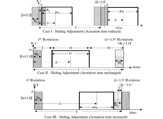
3.4 Phase Adjustment

The system’s actuation becomes non-causal due to the use of PWM control signal. The center of the pulse is to be determined at the end of each rotation; this might lead to the actuation becoming non-causal for some values of A phase adjustment is introduced to effectively produce a causal actuation. An arbitrary threshold zone “ths or the” is chosen

such that the actuation should not fall within this

zone. The observation is always taken at the start of the zone, which slides to deny the actuation to fall within “ths or the”. Table I summarizes the three

possible cases. The Fig.8 shows that for the cases I & III, when the reference is changed for (i+1) rotation, the next observation is so placed as to avoid the system becomes non-causal and align the center of actuation with the reference, but in doing so the actuation time is also changed.

   

 





0

1

1

1 2

1

0 0

0

min , ,

0

i i

i

i

i n

i n

n n

PW i

PW

PW i

PW u T

i

n _{J u J u J u where}

T

i _PW

n u





 

  _



   



   _ 

 



 

 

    

 _{  }  _{ }

 _{   }

 _{ }  _



nN but n0 (10)

Case I - Sliding Adjustment (Actuation time reduced)

Case II - Sliding Adjustment (Actuation time unchanged)

Case III - Sliding Adjustment (Actuation time increased)

3.5 Simulations and Performance Analysis

Simulations were carried out in MATAB and SIMULINK. The parameters used are.

w

_z

=

400

p

rad_sec

,

b

=

400,

K

_i

=

1,

J

=

4

kgm

,

J

_z

=

5

kg

The time interval to complete one revolution is 0.05 sec. The values of parameters are same as in [13], so that fair comparison between thetechniques can be made.The technique [13] shows better transient response but could not track time varying reference as shown in Fig. 9. The PEA based approach [15] though complying constraints (4) shows poor transient response. Though this technique

tracks a time varying signal but with errors and thus not suitable for precise tracking as shown in Fig.10. On the other hand EMC technique has good transient response as well as precisely follows moving reference too. The superior performance of EMC as compared to other techniques can be seen in Fig.11 & Fig.12. MIP & RPA overcome local minima issues where as phase adjustment technique overcomes the causality problem. EMC achieves better settling time for constant reference and is able to track a moving reference effectively. However, the amount of computation required to implement MIP is much more than required in RPA.

Table 1. Possible Scenarios for Phase Adjustment

Case Condition ith Rotation (i+1) th Rotation

I   PW₂ ths

2

s PW

th

   

( ) ( ) end i end i

t



t





( 1) ( )

( 1) ( 1) start i end i

end i start i

t t

t t T



 



 

 _{ } 

 

III  PW₂ the

2 e

PW _th

  

( ) ( ) end i end i

t



t





II Otherwise

t

end i( )



t

end i( )

(a) Fixed Reference (b) Time Varying Reference

Fig. 10. PEA based Stabilization [15]

0 0.1 0.2 0.3 0.4 0.5

-0.5 0 0.5 P o s it io n X -a x is Time

0 0.1 0.2 0.3 0.4 0.5

-1 0 1 P o s it io n Y -a x is Time

0 0.1 0.2 0.3 0.4 0.5

-1 0 1 E rr o r Time

0 0.5 1 1.5 2

-2 0 2 P o s it io n X -a x is Time

0 0.5 1 1.5 2

-1 0 1 P o s it io n Y -a x is Time

0 0.5 1 1.5 2

-1 0 1 E rr o r Time Output Reference X-axis Y -axis

Fig. 11. Stabilization under Fixed & Varying Reference by RPA-EMC

0 0.1 0.2 0.3 0.4 0.5

0 0.5 P o s it io n X -a x is Time

0 0.1 0.2 0.3 0.4 0.5

0 0.5 1 P o s it io n Y -a x is Time

0 0.1 0.2 0.3 0.4 0.5

-1 0 1 E rr o r Time

0 0.5 1 1.5 2

-1 0 1 P o s it io n X -a x is Time

0 0.5 1 1.5 2

-1 0 1 P o s it io n Y -a x is Time

0 0.5 1 1.5 2

-1 0 1 E rr o r Time Output Reference X-axis Y -axis

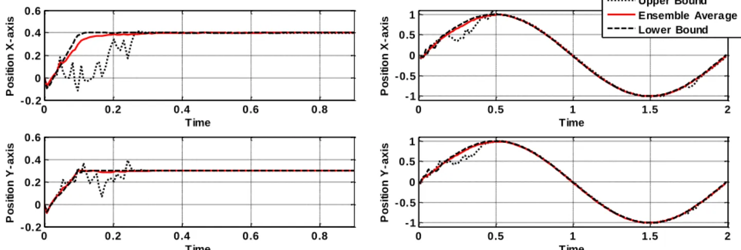
3.6 Monte Carlo Simulations

The robustness of the EMC based control technique is verified by introducing parametric perturbation in the system model (2). Based on the results of over 1200 monte-carlo simulations, both RPA-EMC (Fig. 13) and MIP-EMC (Fig. 14) remained stable with minor variations in settling time and the tracking target was achieved. MIP-EMC showed better settling time as compared to RPA-EMC as they withstand up to 25% of parametric perturbation.

3.7 Real Time Implementation

So far real time implementation of presented algorithms has not been carried out and is out of scope of this paper. However the presented algorithms can be implemented for slow sampling

systems through present day fast processing hardware. Similarly for system with high sampling rate, the presented algorithms can be implemented as offline controllers based on learning control design techniques.

Model predictive control scheme is yet another way by which presented algorithms can be implemented in real time for system having high sampling rate. This technique is being developed by the authors for similar class of systems and will be published in near future.

4. Conclusion

A PWM control design is proposed for the orientation control of an under actuated spinning system under constraints with application on a small drill machine. The scheme is presented to generate

0 0.5 1 1.5 2

-1 -0.5 0 0.5 1 P o s it io n X -a x is Time

0 0.5 1 1.5 2

-1 -0.5 0 0.5 1 P o s it io n Y -a x is Time Upper Bound Ensemble Average Lower Bound

0 0.2 0.4 0.6 0.8

-0.2 0 0.2 0.4 0.6 P o s it io n X -a x is Time

0 0.2 0.4 0.6 0.8

-0.2 0 0.2 0.4 0.6 P o s it io n Y -a x is Time

Fig. 13. Orientation Control through RPA-EMC Under 10% Parametric Variation

0 0.2 0.4 0.6 0.8 1

0 0.2 0.4 P o s it io n X -a x is Time

0 0.2 0.4 0.6 0.8 1

0 0.2 0.4 P o s it io n Y -a x is Time

0 0.5 1 1.5 2

-1 0 1 P o s it io n X -a x is Time

0 0.5 1 1.5 2

-1 0 1 P o s it io n Y -a x is Time Upper Bound Ensemble Average Lower Bound

the required actuating signal of fixed amplitude and variable duration. It is based on the discrete equivalent model of the plant. The atypical nature of the control input failed to generate an exact closed form discrete equivalent model. Controller design is improved by introducing an output feedback error minimizing control based on PWM. The algorithm is a subspace trust-region method and finds optimized values of pulse width and amplitude of the control input. The problems of local minima and non-causality were also addressed. The scheme is very effective for fixed references as well as for tracking problems. The PEA based technique [15] has shown satisfactory results under given constraints, but not suitable for precise movements. The monte-carlo simulations show that the EMC technique gives satisfactory performance under both nominal and parameter variations. EMC-MIP technique even outclass EMC-RPA under high parametric variations. The future work may be focused on the smart optimization techniques for reduction in run time as well as using particle filter approach so as to eliminate optimization step.

5. References

[1] C. Criens,F. Willems and M. Steinbuch, “Under actuated air path control of diesel engines for low emissions and high efficiency”, Proceedings of the FISITA World Automotive Congress, Vol. 189, pp 725-737, 2013.

[2] F. Farivar, MA Shoorehdeli, MA Nekoui and M Teshnehlab, “Synchronization of Under actuated

Unknown Heavy Symmetric Chaotic

Gyroscopes via Optimal Gaussian Radial Basis Adaptive Variable Structure Control”, IEEE Transactions on control systems technology, Vol. 21, No. 6, pp. 2374-2379, 2013.

[3] W. Dong, G. Ying Gu, X. Zhu andH. Ding, “Solving the boundary value problem of an

under-actuated quadrotor with subspace

stabilization approach” in Journal of Intelligent

& Robotic Systems, 2014. DOI

10.1007/s10846-014-0161-3.

[4] G. He and Z.Geng, “Dynamics and robust control of an under actuated torsional vibratory gyroscope actuated by electrostatic actuator”,

IEEE/ASME Transactions on Mechatronics, 2014, DOI: 10.1109/TMECH.2014.2350535. [5] Y. Sagara and N. Hori, “Experimental

verification of roll-angle control using air-jet

pulse actuation”, The 2nd International

Conference on Computer and Automation Engineering (ICCAE), Vol. 5, pp. 418-422, 2010.

[6] J. He, F. Gao andD. Zhang, “Design and performance analysis of a novel parallel servo press with redundant actuation”, International Journal of Mechanics and Materials in Design, Vol. 10, Issue 2, pp 145-163, 2014.

[7] R. E. Andeen, “The principle of equivalent areas”, AIEE Transactions, Vol.79, pp. 332-336, 1960.

[8] T. Sakamoto and N. Hori, “New PWM schemes based on the principle of equivalent areas”, IEEE International Symposium on Industrial Electronics, L'Aquila, Italy, pp. 505-510, 2002. [9] Michael Barr, “Pulse Width Modulation”,

Embedded Systems Programming, September 2001, pp. 103-104.

[10] T. Ieko, Y. Ochi, K. Kanai, N. Hori, and P. N. Nikiforuk, “Design of a pulse-width-modulation spacecraft attitude control system via digital redesign,”, Proc. of IFAC World Congress, Beijing, pp. 355-360,1999.

[11] S.W. Jeon and S. Jung, “Novel analysis of limit cycle for PWM signal of PD control system”, IEICE Electronic Express, Vol 6, No. 11,pp.787-793, 2009.

[12] Tomoaki Suzuki, Toru Ueno and Noriyuki Hori, “Experimental verification of pea-based pwm control using on-off type air-jet thrusters”, Proceedings of the International Conference on Information and Automation, December 15-18, 2005, Colombo, Sri Lanka.

[13] M. B. Malik, F. M. Malik and K. Munawar, “Orientation control of a 3-d under-actuated drill machine based on discrete-time equivalent model”, International Journal of Robotics & Automation, vol. 27, no. 4, 2012, DOI: 10.2316/Journal.206.2012.4.206-3324.

[14] E. Chalupa, “Numeric control drilling jig-multiple-axis aerospace drilling machine”, US Patent No.6419426, issued July 2002.

[15] A. Ali and M. B. Malik, “Pulse Equivalent Area based Orientation of a Class of Under-Actuated System under Constraints”, Accepted, Under publishing in Mehran University Research Journal Of Engineering & Technology.

[16] H. Nisar, A.S. Malik and T.S.Choi, “Multiple initial point prediction based block motion estimation algorithm”, IEEE Symposium on Consumer Electronics, pp 1-6, 2007.

[17] Lei Fan, Xiyang Liu and Liping Jia, “A minimum elimination escape function method

for multimodal optimization problems”, Tenth International Conference on Computational Intelligence and Security” pp.312-216, 2014 [18] P. H. Savet, “Gyroscopes Theory and Design

With applications to Instrumentation, Guidance and Control”, McGraw-Hill Book Company, 1961

[19] J.E. Dennis, “Nonlinear least-squares state of the art in numerical analysis”, Academic

Press, pp. 269-312,1977.

[20] T.F. Coleman and Li.Yi, “ An interior, trust region approach for nonlinear minimization subject to bounds”, SIAM Journal on Optimization, Vol. 6, pp. 418–445, 1996. [21] W. J. Rugh, Linear system theory, 2nd Edition,

(Prentice Hall), 1996.

[22] F. M. Malik, “Sampled-Data Control Based On

Discrete-Time Equivalent Model”, PhD

Dissertation, National University of Sciences and Technology, 2009

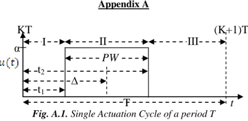
Appendix A

(K+1)T

KT

t

PW

W

α

I

III

∆

II

T

t

1

t

2

Fig. A.1. Single Actuation Cycle of a period T

1. Discrete Time Equivalent Model for EMC

The discrete time equivalent model is developed by considering the characteristics of the constrained control input (Fig. 4). The time interval



KT K,( 1)T



is considered as one revolution of the rotor frame. This time period T is divided into three separate intervals, i.e., interval I, II and III as shown in the Fig.A.1 (Fig.4 is redrawn as Fig.A.1). It must be noted that during intervals I and III the system is un-actuated.

1.1.Interval I: t , where t1 1

2 PW KTKT   

In this interval the system is un-actuated, hence the states of (3) are given [21] by





t1

 

1

t

A

x KT





e x KT

(A.1)

1.2.Interval II: t1 t , where t2 2

2 PW KT KT   

In this interval the system is actuated, using the result in (A.1) as the initial condition, the states of the given system during this interval are









2  

_{ }

2 2 1

1

t t ( t -t )

2 1

t

t t

KT A KT A

KT

x KT e x KT e  Bu  d



  

   

_

(A.2)

Putting value of x KT



t1



from A.1 into A.2, we have





 

2

 

2 2

1

t

t ( t )

2

t

t

KT

A A KT

KT

x KT e x KT e  Bu  d



 



  

_

(A.3)

1.3.Interval III:KTt₂(K1)T

The system is un-actuated in this interval and the states are









 t2

_

_

2

1 A T t

x K T e  x KT (A.4)

Substituting (A.3) in (A.4)









 

2

 

1

(K 1) t

t

1

KT

KT

AT AT A

x K T e x KT e e Bu  d





 