Sharif University of Technology
Scientia IranicaTransactions A: Civil Engineering www.scientiairanica.com
Sensitivity to progressive damage of modal parameters
of an elastic beam: Experimental and numerical
simulation
A. Joghataie
and A. Banihashem
Department of Civil Engineering, Sharif University of Technology, Tehran, Iran.
Received 20 November 2013; received in revised form 8 March 2014; accepted 11 August 2014
KEYWORDS Progressive damage; Aluminum beam; Modal testing; FRF;
Numerical simulation; MAC;
COMAC.
Abstract.The aim of this article is twofold: (1) To provide more insight into the pattern of changes in modal parameters, including natural frequencies and mode shapes, of beams and girders resulting from the increasing of damage level, and (2) Verication of numerical modelling of the problem using data from experiments on an Aluminum box beam. To this end, rst an impact hammer test has been conducted on the 2.6 meter long single span aluminum beam while a progressive damage has been applied at several stages. The modal parameters of the undamaged and damaged beam at dierent intensities have been extracted, and the trend of their changes with respect to the increase in damage level has been studied. Then this process has been simulated numerically by Dynamic Finite Elements Method (DFEM) and the modal parameters have been extracted from numerical simulation. Finally the similarity between the experimental and numerical results has been investigated. The results show that at low levels of damage, the modal parameters change very slightly, especially when just a part of the ange has been damaged, but when the damage has been extended to penetrate the beam web, the modal parameters have shown considerable sensitivity to the damage. Also the sensitivity of the dierent modes to damage has not been the same, though relatively good agreement has been observed between the trend of changes in the modal parameters obtained from experimental and numerical studies, except for a number of modal parameters at very extensive damage level.
© 2015 Sharif University of Technology. All rights reserved.
1. Introduction
The important issue of inspection and health mon-itoring of structures is still attracting considerable attention of the researchers and practitioners all over the world. A detailed review of damage detection techniques has been reported by Doebling et al. [1] and Sooh et al. [2]. Salawu [3] has reviewed the studies on damage identication by monitoring the changes in modal frequencies. Many damage detection studies
*. Corresponding author. Tel.: +98 21 66164216; Fax: +98 21 66014828
E-mail address: [email protected] (A. Joghataie)
have used one or more criteria to evaluate the damage from the change in modal shapes before and after the damage has occurred. For example, Pandey et al. [4] have used the change in modal curvatures as a measure to identify damage. Ricci et al. [5] tried to localize damage with best achievable eigenvector method. Shi et al. [6] have proposed a method to detect damage based on modal strain energy change. Ndambi et al. [7] have compared several classical identication methods for damage detection in a reinforced concrete beam including the change in the natural frequencies and mode shapes, modal strain energy and exibility matrix methods. Maia et al. [8] have compared several damage detection methods, which are based
on changes in modal shapes and Frequency Response Functions (FRFs). Teughels et al. [9] have applied the nite elements model updating methods to determined damage in a 3 span concrete bridge. Catbas et al. [10] have assessed the capabilities of the modal exibility method in the detection of damage in a 3 span steel bridge. Choi et al. [11] have modied the methods of change in mode shape curvatures and dynamic exibility to identify damage in a timber beam. Dixit et al. [12] have proposed a new strain energy based method to analytically determine the location and extend of damage in a beam.
Recently, some authors have reported the success-ful application of intelligent computational methods in damage identication problems. Huang et al. [13] have implemented articial neural networks for damage detection of structures in two stages where rst a neural network is trained to identify the parameters of the structure both with and without damage, next the obtained results are used to identify the probable location and extent of damage. Perera et al. [14] have applied Genetic Algorithms (GA) to identify the extent and location of damage using changes in modal parameters including natural modal frequencies and mode shapes.
Other new techniques have been proposed and utilized for damage identication and health monitor-ing of structures too; for example wavelet transform has been used by Hou et al. [15]. In the eld of experimental identication of structures, Morassi et al. [16] have used dynamic vibration techniques to identify the parameters of a three span post-tensioned reinforced concrete bridge.
In modal analysis, some criteria have been pro-posed by the researchers to compare the mode shapes before and after damage. Two of the commonly used criteria have been Modal Assurance Criteria (MAC) and Coordinated Modal Assurance Criteria (COMAC) values [17]. Vandawaker et al. [18] have compared the mode shapes of a partially constrained plate before and after damage using MAC. Zang et al. [19] have dened a new correlation function, similar to MAC, to directly compare the frequency response functions to determine damage.
Generally, tests on structural systems, such as beams, are costly both considering time and expense. Hence numerical simulation is an essential approach to study the behavior of structures and structural ele-ments; so the precision of numerical simulation which should be veried is vital to its success. Simulation of damage by nite element method provides valuable information about the precision of detection methods and success of new methods which are proposed every now and then. Many studies on Finite Element (FE) simulation of health monitoring and damage detection of beams have been reported in the past, such as
Pothisiri et al. [20] and Weng et al. [21]. Farrar et al. [22,23] have compared some of the damage detection techniques on a steel bridge by applying a progressive damage to one of its girders. In all of these studies, numerical simulation was either a tool for damage detection, or for comparison between numerical and experimental damage detection. But the trend of changes in the modal parameters due to a progressive damage and also the accuracy of numerical modeling were not of much interest though more knowledge about these two subjects can be very useful to improve the model based damage detection techniques. In this paper, it has been desired to assess the precision of nite element simulation of forced vibration identi-cation of progressive damage in an aluminum beam by comparison with the results obtained from experiments on a real beam of the same geometric properties. The beam has been built and tested at the structural laboratory of the Civil Engineering Department of Sharif University of Technology, Tehran, Iran.
The beam is a 2.6 meter long single span alu-minum with hollow rectangular cross section, sitting on two supports providing xed conditions.
The very common criteria for damage detection have been Frequencies Changes, MAC (Modal Assur-ance Criteria) and COMAC (Coordinated MAC). But regardless of the type of structures, a main problem with forced and ambient vibration detection methods using the above criteria has been that they are not sensitive to early stage damage, and hence they cannot provide helpful information about the damage until it has become severe. Hence another objective of this paper has been to test how sensitive these criteria to damage intensity are.
Laboratory experiments: At the rst stage, the damage has been applied to the aluminum beam in three levels by drilling one, three and ve small holes in its top ange where the intensity of damage has been increased by increasing the number of holes. In the second stage, the top ange has been cut to its full depth and nally the web has been cut to the bottom ange in 6 stages from top to bottom to simulate a severe progressive damage. Forced vibration tests have been conducted at the dierent levels of damage where the input and corresponding response have been collected and processed. Three simple traditional but widely used methods of damage assessment including the changes in natural frequencies, MAC and COMAC of the mode shapes have been used to draw conclusion about the intensity and location of the damage. The results have been reported in the following sections.
Finite element simulations: Next, a linear nite element model of the same aluminum beam has been
prepared and tested numerically. The modal properties of the beam model have not been extracted by solving its eigenvalue problem, but impact hammer test has been simulated and the dynamic response of the beam as well as the impact force time history have been used to determine the FRFs of the beam. Then, the modal properties of the beam have been extracted from its FRFs similar to what was done for the tests. A progressive damage similar to, but obviously not exactly the same as, what has been done in the experiment has been applied to the beam. The results of the simulations have been reported in the following sections.
In the following sections, rst, the theory of modal analysis methods has been explained briey. Next, the tests conducted on the experimental beam model, subjected to progressive damage, have been explained. Then the nite element simulations of the tests have been reported. Finally the results are discussed including comparison between the tests and Finite Elements simulations, followed by conclusions.
2. Theory
2.1. Frequency response function
The equation of motion of a dynamical system is as follows:
mx(t) + c _x(t) + kx(t) = f(t); (1) where t is time, k, m and c are stiness, mass and damping matrices of the system, respectively, and f(t) and x(t) are applied load and nodal displacement vectors, respectively. Under a harmonic loading, we have:
x(t) = X(!)ei!t and f(t) = F(!)ei!t; (2)
where X and F are amplitudes of displacement and force vectors, which can be complex, and ! is the ex-citation frequency. Also \i" represents unit imaginary number. Hence, we get:
X =k + i!c !2m 1F; (3)
where:
(!) =k + i!c !2m 1; (4)
is the structure receptance or dynamic compliance. For n degrees of freedom, (!) is an n n matrix. The elements of the Frequency Response Function (FRF) matrix are as follows:
jk(!) = nm
X
r=1
'jr'kr
(!2
r !2) + i(2!!rr); (5)
where jkis the element jk of the FRF matrix, ' is the
normalized mode shape matrix with respect to the mass matrix, j and k are node numbers, r is mode number, nmis the number of modes, and !rand rare natural
frequency and modal damping ratio corresponding to the rth mode, respectively. Recalling that if the two nodes, at which the excitation is applied and where the response is measured, are the same, the corresponding frequency response function is called the \point FRF" while if the nodes are dierent, it is called a \transfer FRF" [17,24].
In practice, the frequency response function can be obtained by applying excitations at dierent fre-quencies or by the application of a single excitation containing a broad range of frequencies, and recording the response. Then element ij of the FRF matrix can be determined as:
ij= XFi(!)
j(!); (6)
where Fj(!) and Xi(!) are Fourier transforms of
the applied load at the jth degree of freedom, and recorded displacement at the ith degree of freedom, respectively [17,24].
2.2. Extraction of modal parameters
Dierent methods have been proposed for determina-tion of modal parameters including natural frequencies, modal damping ratios and mode shapes. The peak picking, used in this paper too, has been one of the most commonly used methods [17,24]. The method is especially suitable and precise enough for low damping structures with very distinguishable natural frequen-cies.
The peak picking method: In this method, the natural frequencies are identied as the frequencies at which the peaks of amplitude occur. The modal damping ratios are also determined by the half power method. Knowing natural frequencies and damping ratios, the mode shapes ('jr) can be determined by
Eq. (5) if an appropriate set of FRFs exist. More details about this method can be found in textbook on modal testing such as [17,24].
2.3. Comparison of modal parameters
The sensitivity of modal frequencies and shapes to damage progression for the aluminium beam has been studied both experimentally and numerically as ex-plained below.
2.3.1. Comparison of modal frequencies
Denoting modal frequency number i corresponding to damage level j by !i;j, i = 1; 2; ::; nm, j = 0; 1; 2; :::; nd,
where nd is total number of damage levels, the modal
frequencies have been normalized by division to the undamaged frequencies as follows:
!0
i;j= !!i;j
i;0; i = 1; 2; :::; nm; j = 0; 1; 2; :::; nd; (7)
where !0
i;j is normalized frequency number, i,
corre-sponding to damage level, j. Consequently !0 i;0 =
1; i = 1; 2; ::; nm.
2.3.2. Comparison of mode shapes
Modal Assurance Criteria (MAC) for comparison of two mode shapes, either from experiments or numerical analysis, is determined from [17]:
MAC( x; y)= j
Pn
j=1( x)j( y)jj2
jPnj=1( x)j( x)jjj
Pn
j=1( y)j( y)jj(8);
where ( x)j and ( y)j are the jth components of the
two mode shape vectors corresponding to the same or two dierent sets of mode shapes, x and y, recalling that n is the number of degrees of freedom and denotes the complex conjugate. MAC=1 when the two mode shape vectors are the same, and MAC=0 when they are normal to one another. In this study, the mode shapes corresponding to each damage level have been compared with the mode shapes of the undamaged beam.
Similar to MAC, COMAC is also a criterion to assess the similarity of mode shapes of the undamaged and damaged beam. However, while MAC returns a matrix, COMAC provides a scalar measure which can be calculated at any point on the beam. COMAC is determined from [17]:
COMAC(i)= j Pnm
r=1( x)ir( y)irj2
jPnm
r=1( x)ir( x)irjjPr=1nm( y)ir( y)irj(9);
in which ( x)ir and ( y)ir are the ith components
of the rth mode shapes vectors corresponding to two dierent sets of mode shapes (here corresponding to the undamaged and damaged beams). Also nm is the
number of extracted mode shapes and denotes the complex conjugate of the vector.
3. Experimental study 3.1. Experimental setup
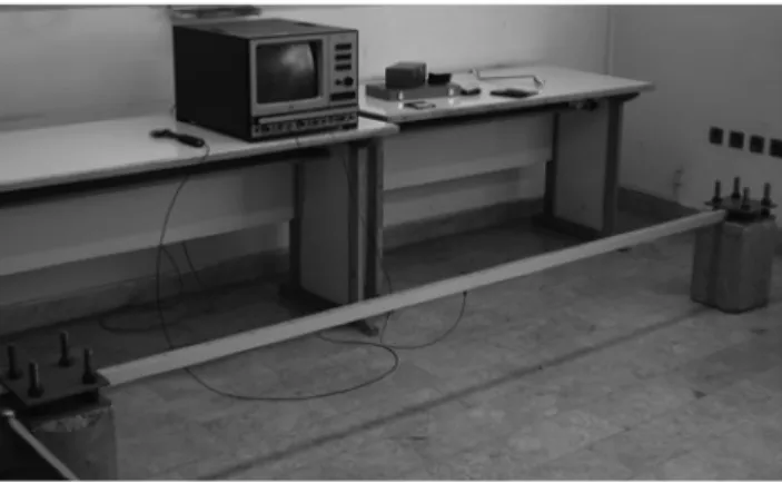
The beam studies has been a 3 m long square box aluminum beam, of dimensions 3:55 3:55 0:15 cm, xed at both ends. Figure 1 shows the test set up. The supports have been concrete blocks of dimensions 25 25 35 cm. Two 20 20 1 cm steel plates have been used to provide xed end supports. The beam has been placed on the supports and was xed by using 4 bolts, which have been embedded in the concrete blocks, as shown in Figure 1. Two rubber pads have been placed between the beam and the upper and lower plates in each support to distribute the contact force
Figure 1. Experimental setup.
between them and to provide better xity conditions. Noticing 20 cm of each end of the beam has been sitting on the supports, the free span of the beam has been 260 cm long.
Twenty one points have been marked on the top ange of the beam. Also the two beam end points have been numbered 22 and 23 as shown in Figure 2.
An impact hammer, where a force transducer with sensitivity of 3.93 pC/N has been attached to it, has been used for forced vibration tests. The total mass of the hammer has been about 280 gr. The hammer tip was changeable and could be from steel, plastic or rubber. Since it was desired to excite a larger number of modes, a steel tip has been used because more exible tips could provide narrower band frequency ranges. Im-pact to the beam by the hammer has been applied only at points 1 to 21. A piezoelectric accelerometer with the following characteristics: Sensitivity of 9.8 pC/g, mounted response frequency of 42 KHz and weight of 11 gr, has been placed at point 10 in order to measure the response through the time. A dual channel analyzer has been used for data acquisition.
3.2. Forced vibration test procedure
The damage has been applied to the beam at 80 cm from the right support (between points 15 and 16) at rst by drilling 5 holes of 3 mm diameter in the top ange of the beam and then by cutting the top ange and the both side webs. The holes have been drilled symmetrically with respect to the center of the beam. To determine a suitable point to mount the accelerometer, the rst 10 mode shapes of the xed end beam were numerically identied by solving the eigen-problem; where point 10 located at 6.5 cm from the mid span has been chosen for response measurement because it was expected that none of the rst 10 exural mode shapes would have a zero value at this point. After each level of damage has been applied, the beam has been tested by applying impact at all the points while measuring the acceleration at point 10 through the time. The data was collected at a rate of 4000 samples/s. The scenario for applying the damage and
Figure 2. Location of stations on aluminum beam showing distance between points.
Figure 3. Levels of damage during experiments: DL1 (a), DL2 (b), DL3 (c), DL4 (d), DL5 (e), DL6 (f), DL7 (g), DL8 (h), DL9 (i), and DL10 (j).
data acquisition is explained below where DL denotes Damage Level:
1. DL0. Damage Level 0: undamaged beam.
2. DL1. Damage Level 1: at 80 cm from right support, 1 hole, diameter 3 mm, top ange, as shown in Figure 3(a).
3. DL2. Damage Level 2: at 80 cm from right support, 3 holes, diameter 3 mm, top ange, as shown in Figure 3(b).
4. DL3. Damage Level 3: at 80 cm from right support, 5 holes, diameter 3 mm, top ange, as shown in Figure 3(c).
5. DL4. Damage Level 4: at 80 cm from right support, full thickness of the top ange has been cut, as shown in Figure 3(d).
6. DL5. Damage Level 5: at 80 cm from right support, full thickness of the ange and 5 mm of the webs on both sides of the section have been cut, as shown in Figure 3(e).
7. DL6. Damage Level 6: at 80 cm from right support, full thickness of the ange and 10 mm of the webs on both sides of the section have been cut, as shown in Figure 3(f).
8. DL7. Damage Level 7: at 80 cm from right support, full thickness of the ange and 15 mm of the webs on both sides of the section have been cut, as shown in Figure 3(g).
9. DL8. Damage Level 8: at 80 cm from right support, full thickness of the ange and 20 mm of the webs
on both sides of the section have been cut, as shown in Figure 3(h).
10. DL9. Damage Level 9: at 80 cm from right support, full thickness of the ange and 25 mm of the webs on both sides of the section have been cut, as shown in Figure 3(i).
11. DL10. Damage Level 10: at 80 cm from right support, full thickness of the ange and 30 mm of the webs on both sides of the section have been cut, as shown in Figure 3(j).
3.3. FRFs from experiments
To reduce as much as possible the eect of noise from uncontrolled sources, for each damage level, 3 impact hammer tests have been run for each station which their corresponding FRF values have been determined and their average has been considered as the result.
Figure 4 shows two samples of the recorded frequency response functions for the undamaged beam. The solid line represents point 10 FRF while the dotted line represents the transfer or cross FRF where the beam has been hit at point 3, and the response has been measured at point 10. The FRFs have been calculated by dividing the FFT of response (here acceleration) by the FFT of impact force.
3.4. Extracting modal parameters from the records of impact hammer tests
The modal parameters have been determined using peak picking method which has been explained in the previous sections. The following paragraphs explain the results.
Table 1. The rst 7 modal frequencies (Hz) of the undamaged (DL0) and 10 damaged beam scenarios.
Mode no. DL0 DL1 DL2 DL3 DL4 DL5 DL6 DL7 DL8 DL9 DL10
1 34.23 34.28 34.21 34.21 34.10 34.02 33.84 33.59 33.12 32.47 32.05 2 95.09 95.16 94.98 94.95 94.47 93.87 92.53 90.19 86.03 78.78 70.58 3 184.44 184.61 184.31 184.25 183.93 183.61 183.00 182.29 181.23 179.86 178.76 4 303.84 304.31 303.81 303.70 302.86 302.23 300.76 299.05 29 6.41 291.94 288.08 5 449.26 447.51 446.43 446.36 444.12 441.30 435.04 426.58 41 5.95 402.53 391.45 6 621.37 622.15 621.17 620.95 618.57 617.02 613.66 609.69 60 4.72 599.05 595.01 7 805.34 806.54 805.03 804.66 802.04 802.57 801.68 799.77 796.68 791.81 787.44
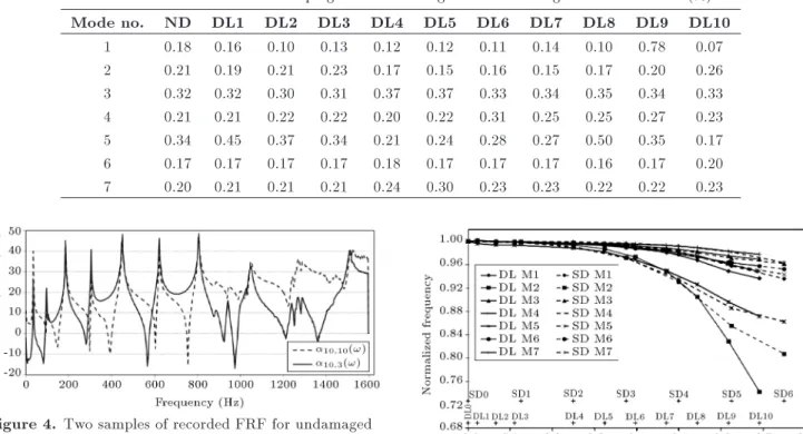
Table 2. The rst 7 modal damping of the undamaged and 10 damaged beam scenarios (%).
Mode no. ND DL1 DL2 DL3 DL4 DL5 DL6 DL7 DL8 DL9 DL10
1 0.18 0.16 0.10 0.13 0.12 0.12 0.11 0.14 0.10 0.78 0.07 2 0.21 0.19 0.21 0.23 0.17 0.15 0.16 0.15 0.17 0.20 0.26 3 0.32 0.32 0.30 0.31 0.37 0.37 0.33 0.34 0.35 0.34 0.33 4 0.21 0.21 0.22 0.22 0.20 0.22 0.31 0.25 0.25 0.27 0.23 5 0.34 0.45 0.37 0.34 0.21 0.24 0.28 0.27 0.50 0.35 0.17 6 0.17 0.17 0.17 0.17 0.18 0.17 0.17 0.17 0.16 0.17 0.20 7 0.20 0.21 0.21 0.21 0.24 0.30 0.23 0.23 0.22 0.22 0.23
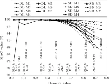
Figure 4. Two samples of recorded FRF for undamaged beam.
Modal shapes, frequencies and damping ratios: For each damage level, only the rst 7 mode shapes in the frequency range of 0-1600 Hz were of appropriate quality to extract. Tables 1 and 2 contain details about the modal frequencies and damping ratios for the rst 7 modes of vibration corresponding to the undamaged and the 10 scenarios of progressive damage. As the theory predicts, the frequencies have decreased monotonically with increasing the damage, because of stiness reduction. Also the modal damping ratio has varied from 0.07% to 1.28% which shows the beam damping has been low.
3.5. Eect of progressive damage on modal frequencies and damping
For comparison of modal frequencies corresponding to the undamaged and damaged beams, rst the frequencies have been normalized according to Eq. (7). In Figure 5, which also contains information from the next sections of this paper, the solid lines plot
Figure 5. Variation of the rst 7 normalized exural modal frequencies versus damage value, plotted separately for each mode from tests and FE simulations.
the normalized frequency values for each mode from experiments versus damage level. Each curve belongs to a specic mode number. The beam has become softer with increase of damage, and hence all the normalized modal frequencies have decreased. As expected, for all the modes, at low damage levels, the normalized frequencies have not changed considerably from 1 which corresponds to the undamaged normal-ized frequency. This low sensitivity to minor damage is observed for up to Damage Level 3 (DL3), which corresponds to damage caused by drilling holes in the top ange only, where 5 holes have been drilled for DL3. However after damage level 3, where more damage has been applied to the beam, the modal frequencies have shown higher sensitivity to the damage level. Noticing the damage location has been at 80 cm from the right
Figure 6. Changes of damping ratios with increasing damage level.
support, between points 15 and 16, it was expected that the modes, whose mode shapes had a node close to the damage location, be less sensitive to the damage, while the modes whose mode shapes had an antinode at the damage location be more sensitive [1]. This conclusion has been generally correct for this study too, since mode shapes number 2 and 5, which have antinodes near the damage location, have experienced more changes in natural frequencies, while modes 7, 3 and 6, which have nodes near the damage location, have experienced less changes. This has been noticed by Farrar et al. [22] too, who conducted a similar experiment on a girder of a bridge.
Figure 6 shows the change in the modal damping as a result of damage. No direct conclusion can be drawn about damage level with modal damping. The sharp change from DL8 to DL9 may point to some source of error in the data corresponding to mode 1 at DL9.
3.6. Eect of progressive damage on mode shapes
3.6.1. MAC for comparison of mode shapes
With the rst 7 modes, 49 MAC values have been calcu-lated when comparing the mode shapes of undamaged beam with any one of the 10 damage levels.
Though all the elements of MAC can be important in the assessment of damage, it is common to only compare the diagonal elements which are the MAC values corresponding to similar mode shapes of the undamaged and damaged beams. Hence, in this study, only the 7 diagonal MAC values have been used in the assessment of damage.
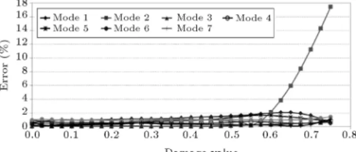
In Figure 7, which also contains information from the next sections of this paper, the solid lines show the variation of diagonal MAC values of experimental mode shapes versus damage level where the vertical axis shows the MAC value and the horizontal axis represents the damage level. Each curve belongs to a specic mode. As can be seen, except for the fth mode shape of DL1, where there might have been some error
Figure 7. Variation of MAC values corresponding to rst 7 mode shapes versus damage value, plotted separately for each mode from tests and FE simulations.
in the recorded data, as discussed before, the MAC values have reduced monotonically with increasing damage level up to DL10. This reduction in the MAC values with increasing damage is meaningful because it indicates that the similarity between damaged and undamaged mode shapes has reduced as a result of increasing damage.
It is noteworthy that the mode shapes which have shown the most changes, corresponding to the largest MAC values, are not necessarily associated with the mode shapes whose modal frequencies have changed signicantly. This can be seen by referring to Figure 5 where modal frequency No. 2 has changed more than that of mode No. 7, though the MAC value for mode 7 has been larger. Meanwhile several researchers such as Farrar et al. [22] believe that signicant changes in MAC values do not occur in those modes which have nodes near damage location.
3.6.2. COMAC for comparison of mode shapes Figure 8 shows COMAC values over the length of the beam, calculated based on the 7 mode shapes, used for comparison of the undamaged beam and the beam with dierent levels of damage. Each curve has been drawn for a specic damage level. As can be seen, in most of the cases, as the level of damage has increased, lower values have been obtained for COMAC, and the curve has shifted downwards. However noticing the gure, this cannot be generalized in that there are some violations of this rule and hence no direct conclusion could be drawn neither about the location nor the extent of damage from COMAC values.
4. Numerical simulation
A progressive damage similar to, but not exactly the same as, what has been applied in the
experi-Figure 8. Changes of COMAC criteria (w.r.t.
undamaged modes) along beam length in dierent levels of damage.
ment has been applied to the numerical beam. The modal properties of the numerical beam has not been determined by solving an eigenvalue problem but similar to the experiment, the impact hammer test has been simulated and the components of the dynamic response of the beam have been used to determine the frequency response functions of the beam based on which its modal properties have been extracted.
4-node shell elements have been used for the simulation of the beam. The mass and stiness matrices have been obtained by assembling the mass and stiness matrices of the 4-node shell elements. The damping matrix has been assumed as proportional to the mass and stiness matrices using Rayleigh damping.
Six progressive damage levels have been applied to the beam at the location shown in Figure 9(a).
Denoting Simulated Damage by \SD", the SD levels have been as follows:
1. SD0: undamaged beam, as shown in Figure 9(b).
2. SD1: half of the width of the top ange of the beam has been cut down to its full depth as shown in Figure 9(c), where the length (thickness) of the cut has been 3 mm.
3. SD2: similar to SD1, but the total width of the top ange has been cut. Again the full depth of the ange and 3 mm length has been cut, as shown in Figure 9(d).
4. SD3: In addition to cutting the total width of the top ange, 1/4th of the web depth on both sides has been cut, as shown in Figure 9(e).
5. SD4: In addition to cutting the total width of the top ange, 1/2 of the web depth on both sides has been cut, as shown in Figure 9(f).
6. SD5: In addition to cutting the total width of the top ange, 3/4th of the web depth on both sides has been cut, as shown in Figure 9(g).
7. SD6: In addition to cutting the total width of the top ange, the whole web depth on both sides has been cut, as shown in Figure 9(h).
The damage levels SD0 and SD2 can be consid-ered as simulating the damage levels DL0 and DL4 in experiments respectively, while SD1, SD3, SD4 and SD5 cannot be considered as exact counterparts of DL1 to DL3 and DL5 to DL10.
4.1. Impact hammer simulation and dynamic analysis
The impact hammer load has been assumed a triangu-lar function of time (Figure 9(i)) where the duration and amplitude have been 0.25 milliseconds and 250 N,
Figure 9. FE mesh of beam and time history of excitation: (a) beam and boundary conditions; (b) SD0; (c) SD1; (d) SD2; (e) SD3; (f) SD4; (g) SD5; (h) SD6; and (i) time history of exciting force.
Table 3. The rst 7 modal frequencies (Hz) of the undamaged and 6 damaged beam scenarios in the numerical simulation.
Mode no. SD0 SD1 SD2 SD3 SD4 SD5 SD6
1 34.54 34.53 34.48 34.32 33.95 33.08 32.32 2 94.72 94.54 93.86 92.08 88.12 80.98 76.43 3 184.39 184.31 184.02 183.27 181.69 179.09 177.31 4 302.10 301.94 301.37 299.83 296.34 289.91 284.94 5 446.43 445.48 442.08 433.61 417.20 395.23 384.93 6 615.50 615.00 613.26 609.14 601.85 592.89 586.16 7 807.15 807.00 806.39 804.77 800.90 792.58 777.78 8 1019.0 1017.2 1010.8 996.63 977.61 966.53 964.98 9 1247.8 1246.6 1242.1 1232.6 1218.9 1206.4 1193.1 10 1490.4 1490.4 1490.1 1489.3 1487.5 1483.4 1449.1
respectively. Also to reduce the number of computer runs, the beam was hit at point 10, at 6.5 cm from the middle of the beam, while recording the response at dierent points in just a single run. The total time of analysis for each damage level has been 1 second. New-mark's method has been used. According to Nyquist-Shannon sampling theorem [25] for the frequency range of interest, 1 to 1600 Hz, the minimum sampling rate should be 3200 Hz (sampling time t = 0:3125 milliseconds). Hence the sampling and integration time increments equal to 0.025 milliseconds have been used. 4.2. Calculating Frequency Response
Functions (FRFs)
Applying the impact, the vertical displacements at the 21 points on the beam corresponding to SD0 to SD6 have been used to determine the FRFs according to Eq. (6) and noticing j = 10:
i;10(!) = FXi(!)
10(!); i = 1 to 21; (10)
where only one column of the FRF matrix has been computed which is necessary and sucient to extract the modal parameters.
Since there are always sources noise in tests, an articial noise was generated using Gaussian ran-dom numbers, and added to the displacement vector. Arbitrarily 0.25% of the maximum amplitude of the computed displacement at each of the stations, and also the impact force at station No. 10 were added. However this could be a subject of more studies.
For the purpose of illustration, Figure 10 shows the calculated FRF of the displacement at point 10 (Figure 2) in the undamaged case, both with and without noise.
4.3. Determination of modal properties using peak picking method
Since the FRFs from numerical simulation have been calculated for the vertical displacements, then all of
Figure 10. 10;10(!) for numerical model of undamaged
beam, with (dotted line) and without (solid line) added noise.
the extracted modal parameters belong to the vertical exural modes which have been the interest of this research. Table 3 contains information about the 10 calculated modal frequencies corresponding to the 7 damage levels SD0 to SD6. Also the dashed lines in Figure 5 show the change in the normalized frequencies of the simulated beams as the result of increasing damage, calculated by Eq. (7).
4.4. Calculating MAC and COMAC values The dashed lines in Figure 7 show the changes in MAC values for the rst 10 exural modes of the numerical model before and after damages have been applied. While it might be expected that the modes with larger changes in their frequencies show larger MAC values too, the results do not support this idea for all the modes. For example, while the 7th mode has shown the minimum sensitivity of frequency to changes in damage extent, its MAC has shown the highest sensitivity to the damage. Contrary to mode 7, mode 2 has shown the highest and lowest sensitivities of frequency and MAC to damage extent, respectively.
Figure 11 shows the COMAC values correspond-ing to the rst 10 exural modes of the undam-aged and damundam-aged numerical models. Similar to the experiments, it has not been possible to correlate
Figure 11. Changes of COMAC values along beam length for dierent damage levels.
Figure 12. Mode shapes of experimental (solid lines) and simulated (dashed lines) undamaged beams: (a) Mode 1; (b) mode 2; (c) mode 3; (d) mode 4; (e) mode 5; (f) mode 6; and (g) mode 7.
the COMAC values to the damage extent and loca-tion.
5. Precision of FE simulation by comparison to test results
5.1. Undamaged beam
First the results from test and simulation of undamaged beam have been compared. Table 4 compares the rst seven modal frequencies while Figure 12 compares the rst seven modal shapes of the undamaged beam. The dierence seems practically acceptable.
5.2. Damaged beams
For the purpose of numerical comparison, the extent of damage has been quantied as the percent loss of the total cross sectional area of the beam and has been called \damage value". Table 5 tabulates the damage value for each damage level in the experiments and FE simulations.
5.2.1. Comparison of modal frequencies
Figure 5 shows the changes in the normalized natural frequencies, corresponding to the rst 7 exural modes of the beam against damage value, both for the tests and numerical simulations. The frequencies have been normalized in accordance with Eq. (7). Also to provide a better image of the problem, the damage value corresponding to each damage level, as reported in Table 5, has been marked in the gure by \+" signs. As can be seen, the normalized natural frequencies from tests and simulations are very close to one another for all the modes. Also the percentage of dierence between the normalized frequencies from tests and FE simulations plotted in Figure 13, has been calculated from the following equation:
m(dv) =jftm(dv) fsft m(dv)j m(dv)
m = mode number = 1; 2; :::; 7; (11) where dv is the damage value, m(dv), ftm(dv) and
Figure 13. Error% in normalized modal frequencies from simulations compared with tests.
Table 4. Natural frequencies (Hz) of undamaged beam in experimental and numerical simulation. Mode no. Mode 1 Mode 2 Mode 3 Mode 4 Mode 5 Mode 6 Mode 7
DL0 34.23 95.09 184.44 303.84 449.26 621.37 805.3
SD0 34.54 94.72 184.39 302.10 446.43 615.50 807.2
Table 5. Damage value corresponding to each damage level in experiments and simulations.
Experiments Damage level DL0 DL1 DL2 DL3 DL4 DL5 DL6 DL7 DL8 DL9 DL10 Damage value 0 0.022 0.066 0.110 0.250 0.324 0.397 0.471 0.544 0.618 0.691
Simulations Damage level SD0 SD1 SD2 SD 3 SD4 SD5 SD6
fsm(dv) are the percent of change in normalized
frequency and normalized frequencies from test and numerical simulation for mode m, respectively, as functions of damage value. To draw the curves, the values for 31 equally spaced points on the normalized frequency curves in Figure 5 have been measured and used in Eq. (11). The error is below 1.1% for all the modes except for mode shape 2 where the error is relatively high for higher levels of damage. Depending on the precision required, the percent dierence can be evaluated as acceptable or not. For damage detection purposes in structural engineering, it seems practically acceptable while only for the rst and second modes the dierence might be considered as noteworthy. There are some probable reasons for the dierences, as explained in a separate section later.
5.2.2. Comparison of MAC values
In Figure 7, each curve represents the MAC value ob-tained from comparison of one of the 7 exural modes of the damaged with its counterpart mode of the un-damaged beam as a function of damage level, both from test (solid curves) and numerical simulations (dashed curves). The pattern of changes in MAC values as the result of increasing damage in both the test and simu-lated beams has been similar. Figure 14, based on the curves in Figure 7, plots the dierence between MAC values from test and FE simulation for each of the 7 modes. The error is more signicant at higher damage levels however, except for mode 5, it may be concluded that in general the dierence is minor and the precision is high enough for structural damage detection. The considerable dierence in mode 5 obtained from tests can be the result of some noise transferred from surroundings to the experimental setup. The probable causes for the dierences in MAC values have been ex-plained in a separate section later. Similar to what was done for Figure 13, the error calculated for 31 equally spaced damaged levels has been used to draw Figure 14. 5.3. Sources of error
Similar to any other simulation problem, the pre-cision in this study has been dependent on factors including the modeling of geometry, introduction of proper boundary conditions and especially the pattern
Figure 14. Error% in MAC values from simulations compared with tests.
of loading. Another source of dierence from real experiment is that it is not possible to model, with high precision, the surrounding noise which can contaminate the data in real experiments and change the results drastically.
In this study, the error of dening proper bound-ary conditions in the simulation seems to be the main source of error. Although it was tried to provide xed end conditions for the test beam as explained in the section on experimental setup, it is expected that there has been some deciencies. The eect of support conditions has been pronounced when damage level has increased because the damage location becomes more and more similar to a hinge, causing large geometric deformation.
In FE simulation, the size of the elements has eect on the precision of the simulation though might not be that signicant. Obviously smaller elements are more suitable to be used in the damage area, as has been done in this study. Another source of simulation error returns to the method of modeling the dynamic response of the beam; for example selection of integration time interval seems to have some eect on the precision of simulation, though minor.
In general, it can be said that although numerical modeling of the tests in this study has ltered the real experiment and has idealized it, rstly, the dierences have been minor and secondly, the trend of changes in the modal properties is almost the same as in experiments and numerical modeling.
6. Conclusions
Noticing numerical simulation, using Finite Element Method is a valuable and economical approach to study the occurrence of damage and their progression in beams, which can be used to evaluate the dierent damage detection methods; the precision of simulation is of essential concern. In this paper, a xed ends box aluminum beam of 2.6 m span was built at the structural engineering laboratory of Sharif University of Technology, and its dynamic response under forced vibration by impact hammer was studied when the beam was subject to progressive damage. To experi-mentally model a progressive damage, the damage was applied to a point on the beam by drilling 5 holes in its top ange where 1, 3 and 5 holes were drilled in 3 consecutive stages. Next, using saw, the top ange was completely cut and then the webs of the box were cut symmetrically in 6 stages. Under each damage level, the impact was applied at a number of selected points on its length while the resulting response was recorded at a given station. The recorded data was then used to determine the modal characteristics of the rst 7 exural modes of the beam, including their frequencies and shapes. The recorded data was used
to determine MAC values for each mode corresponding to each damage level. The obtained MAC values were used to determine how damage had aected the mode shapes of the beam. Since the determination of damage extent and location was not within the objectives of this paper, to focus on the main objective of the paper, which has been the assessment of the precision of numerical simulation of experiments, no comment on damage detection has been included in the paper.
The same procedure of progressive damage model-ing and testmodel-ing usmodel-ing impact hammer was simulated by Finite Element Method, where 2768 numbers of 4-node shell elements were used. The number of degrees of freedom of the system was 16608. For more precision, 1520 elements were used in the damage location and its vicinity and the progressive damage was simulated by removing a determined number of these smaller shell elements. The impact load was simulated by applying a triangular load with the duration of 0.25 ms. The collected numerical data was then used to determine the FRF values from which the modal properties of the rst 10 exural modes of the numerical beam have been extracted in exactly the same way as used in the experiments. The modal frequencies and shapes before and after application of damages were compared and MAC values were determined to compare the eect of damage extent on modal shapes.
The modal frequencies and shapes from tests on the aluminum beam and their FE simulations were compared for all the damage levels where the results show that numerical simulations were able to simulate the tests with enough precision. The maximum dif-ference in natural frequencies of corresponding mode shapes from tests and simulations has been less than 2% and the dierence in MAC values has been less than 3% in general.
The observed minor dierences between the modal parameters of tests and FE simulations have been explained as the results of unpredicted sources of error, such as the surrounding noise as well as imprecision in FE simulation of damage geometry and boundary conditions.
Though this paper was not intended to address issues related to damage identication in beams and it was targeted towards investigating the accuracy of FE simulation of progressive damage in elastic beams (an Aluminum beam has been studied), as expected it was observed that the modal frequencies and MAC values reduced with increasing the damage extent which resulted in the softening, causing more exibility in the beam.
References
1. Doebling, S.W., Farrar, C.R., Prime, M.B. and She-vitz, D.W. \Damage identication and health
mon-itoring of structural and mechanical systems from changes in their vibration characteristics: A literature review", Report LA-13070-MS, Los Alamos National Laboratory (1996).
2. Sooh, H., Farrar, C.R., Hemez, F.M., Shunk, D.D., Stinemates, D.W., Nadler, B.R. and Czarnecki, J.J. \A review of structural health monitoring literature: 1996-2001", Report LA-13976-MS, Los Alamos National Laboratory (2004).
3. Salawu, O.S. \Detection of structural damage through changes in frequency: A review", Eng. Struct., 19, pp. 718-723 (1997).
4. Pandey, A.K., Biswas, M. and Samman, M.M. \Dam-age detection from changes in curvature mode shapes", J. Sound. Vib., 145, pp. 321-332 (1991).
5. Ricci, S. \Best achievable modal eigenvectors in struc-tural damage detection", Exp. Mech., 40, pp. 425-429 (2000).
6. Shi, Z.Y., Law, S.S. and Zhang, L.M. \Structural damage detection from modal strain energy change", J. Eng. Mech., 126, pp. 1216-1223 (2000).
7. Ndambi, J.M., Vantomme, J. and Harri, K. \Damage assessment in reinforced concrete beams using eigen frequencies and mode shape derivatives", Eng. Struct., 24, pp. 501-515 (2002).
8. Maia, N.M.M., Silva, J.M.M. and Almas, E.A.M. \Damage detection in structures: From mode shape to frequency response function methods", Mech. Syst. Signal Process., 17, pp. 489-498 (2003).
9. Teughels, A. and Roeck, G.D. \Structural damage identication of the highway bridge Z24 by FE model updating", J. Sound Vib., 278, pp. 589-610 (2004).
10. Catbas, F.N., Brown, D.L. and Aktan, A.E. \Use of modal exibility for damage detection and condi-tion assessment: Case studies and demonstracondi-tions on large structures", J. Struct. Eng., 132, pp. 1699-1712 (2006).
11. Choi, F.C., Li, J., Samali, B. and Crews, K. \Applica-tion of the modied damage index method to timber beams", Eng. Struct., 30, pp. 1124-1145 (2008).
12. Dixit, A. and Hanagud, S. \Single beam analysis of damaged beams veried using a strain energy based damage measure", Int. J. Solids Struct., 48, pp. 592-602 (2011).
13. Hung, S.L. and Kao, C.Y. \Structural damage detec-tion using the optimal weights of the approximating articial neural networks", Earthq. Eng. Struct. Dyn., 31, pp. 217-234 (2002).
14. Perera, R. and Torres, R. \Structural damage de-tection via modal data with genetic algorithms", J. Struct. Eng., 132, pp. 1491-1501 (2006).
15. Hou, Z., Noori, M. and Amand, R.S. \Wavelet-based approach for structural damage detection", J. Eng. Mech., 126, pp. 677-683 (2000).
16. Morassi, A. and Tonon, S. \Dynamic testing for structural identication of a bridge", J. Bridge Eng., 13, pp. 573-585 (2008).
17. Ewins, D.J., Modal Testing: Theory, Practice and Application, Wiley (2001).
18. Vandawaker, R.M., Palazotto, A.N. and Cobb, R.G. \Damage detection through analysis of modes in a partially constrained plate", J. Aerosp. Eng., 20, pp. 90-96 (2007).
19. Zang, C., Friswell, M.I. and Imregun, M. \Structural health monitoring and damage assessment using fre-quency response correlation criteria", J. Eng. Mech., 133, pp. 981-993 (2007).
20. Pothisiri, T. and Hjelmstad, K.D. \Structural damage detection and assessment from modal response", J. Eng. Mech., 129, pp. 135-145 (2003).
21. Weng, J.H., Loh, D.H. and Yang, J.N. \Experimental study of damage detection by data-driven subspace identication and nite-element model updating", J. Struct. Eng., 135, pp. 1533-1544 (2009).
22. Farrar, C.R. and Jauregui, D.A. \Comparative study of damage identication algorithms applied to a bridge: I. Experiment", Smart Mater. Struct., 7, pp. 704-719 (1998).
23. Farrar, C.R. and Jauregui, D.A. \Comparative study of damage identication algorithms applied to a bridge: II. Numerical study", Smart Mater. Struct., 7, pp. 720-731 (1998).
24. He, J. and Fu, Z.F., Modal Analysis, Butterworth-Heinemann (2001).
25. Oppenheim, A.V. and Schafer, R.W., Discrete-Time Signal Processing, Prentice Hall (2010).
Biographies
Abdolreza Joghataie received his PhD degree from the University of Illinois at Urbana-Champaign, Illi-nois, US and is now a faculty member of the Structural and Earthquake Engineering Group at the Civil Engi-neering Department of Sharif University of Technology, Tehran, Iran. His research is within the elds of struc-tural optimization, intelligent computation, strucstruc-tural control and concrete structures.
Alireza Banihashem was born in 1978 in Gorgan, Iran. He obtained his BS degree in Civil Engineering from Mazandaran University in 2000 and his MS degree in Structural Engineering from Sharif University of Technology in 2002, where he is currently a PhD candi-date. His research interests include: structural system identication, seismic evaluation and rehabilitation of structures, computational and analytical nonlinear solid mechanics.