Benchmark numerical simulations of rarefied non-reacting gas flows using an open-source DSMC code

(1)

ACCEPTED MANUSCRIPT

Benchmark numerical simulations of rarefied

non-reacting gas flows using an open-source DSMC code

Rodrigo C. Palharini1

Instituto de Aeronáutica e Espa¸co, 12228-904 São José dos Campos, SP, Brazil

Craig White2

School of Engineering, University of Glasgow, Glasgow G12 8QQ, UK

Thomas J. Scanlon3_{, Richard E. Brown}5

Department of Mechanical & Aerospace Engineering, University of Strathclyde, Glasgow G1 1XJ, UK

Matthew K. Borg4_{, Jason M. Reese}6

School of Engineering, University of Edinburgh, Edinburgh EH9 3JL, UK

Abstract

Validation and verification represent an important element in the development of

a computational code. The aim is establish both confidence in the algorithm and its suitability for the intended purpose. In this paper, a direct simulation Monte Carlo solver, calleddsmcF oam, is carefully investigated for its ability to solve low and high speed non-reacting gas flows in simple and complex geometries. The test cases are: flow over sharp and truncated flat plates, the Mars Pathfinder probe, a micro-channel with heated internal steps, and a simple micro-channel.

For all the cases investigated, dsmcF oam demonstrates very good agreement with experimental and numerical data available in the literature.

Keywords: DSMC, Benchmark, Open-source, Rarefied gas dynamics,

Aerodynamics, Low/high speed flows.

1_{Postdoctoral Research Fellow, Division of Aerodynamics.} 2_{Lecturer, University of Glasgow.}

3_{Senior Lecturer, James Weir Fluids Laboratory.}

4_{Professor, Centre for Future Air-Space Transportation Technology.} 5_{Lecturer in Mechanical Engineering.}

(2)

ACCEPTED MANUSCRIPT

1. Introduction

The accuracy and reliability of computer predictions is the focus of much study and debate in the fluid dynamics community. Computational codes can only be considered reliable if they pass a through rigorous process of verification

and validation (V&V). In an effort to standardize the V&V process, a significant

5

amount of literature has been produced on the subject, e.g., [1–8]. The present study adopts the V&V definition stated in Ref. [5], i.e.,

Verification: the process of determining that an implemented model is

capable of correctly performing the task it was designed for.

Validation: the process of determining the degree to which a model is an

10

accurate representation of the real world from the perspective of the intended use of the model.

In other words, verification deals with mathematics and numerics; the con-ceptual model that relates to the real world is not an issue. Validation deals with the actual physics and addresses the accuracy of the conceptual model with

15

respect to the real world, i.e., as measured experimentally [4, 6].

In this paper, high and low speed inert gas flows are investigated in sim-ple and comsim-plex geometries using the direct simulation Monte Carlo (DSMC) method [9]. DSMC is the dominant computational technique for numerical investigations of gas flows that fall within the transition-continuum Knudsen

20

number (Kn) range; where

Kn= λ

L, (1)

andλis the mean free path of the gas, andLis a characteristic length scale of the system. When the Knudsen number is small (Kn <0.01), non-equilibrium effects are insignificant and the standard Navier-Stokes-Fourier (NSF) equations can accurately predict the gas behavior. As Kn increases (0.01< Kn <0.1),

25

(3)

ACCEPTED MANUSCRIPT

slip and temperature jump, and the NSF equations with slip and jump

bound-ary conditions can still be used effectively. However, once the Knudsen number increases into the transition-continuum (0.1 < Kn < 10) and free-molecular

30

(Kn >10) regimes, the NSF equations cannot predict the gas behavior. Re-course to solutions of the Boltzmann equation must be made, and DSMC has proven to be the most reliable method for this purpose in the transition regime, where non-equilibrium effects dominate the gas behavior but inter-molecular

col-lisions are still important. Different forms of Knudsen number can be required

35

to predict different types of continuum breakdown, e.g., a Knudsen number based on local flow gradient lengths can be used across shock waves [10–12].

This paper is intended to be an extension of the DSMC code and results published by Scanlonet al. [13], and demonstrates new developments and ca-pabilities of thedsmcF oamcode.

40

2. Code development and new features

DSMC is a stochastic particle-based method that provides a solution to the Boltzmann equation by emulating the physics of a real gas. A discrete set of simulator particles are tracked in time and space as they interact with each other

and the boundaries of the simulation domain. Particle movements are handled

45

deterministically according to the local time step and their velocity vectors. Once all movements have been completed, inter-molecular collisions are calcu-lated in a stochastic manner in numerical cells. The first key assumption of the method is that a single DSMC simulator particle can represent any number of real atoms or molecules. This can drastically reduce the computational expense

50

of a simulation. Second, it is assumed that particle movements and collisions can be decoupled, which increases the allowable time-step size by several orders of magnitude in comparison with fully-deterministic particle methods, such as molecular dynamics.

The dsmcF oam code is employed in the current paper to solve rarefied

55

(4)

ACCEPTED MANUSCRIPT

Pathfinder probe, and pressure-driven flow in microchannels. This new

free-ware, based on Bird’s algorithms, has been developed within the framework of the open-source computational fluid dynamics toolbox OpenFOAM [14], in conjunction with researchers at the University of Strathclyde, as described in

60

Ref. [13]. Recent dsmcF oam code improvements [15, 16] not described in Ref. [13] include: a robust measurement framework, vibrational molecular en-ergy, the quantum-kinetic (QK) chemistry model [17], and new boundary

con-ditions, such as implicit, prescribed pressure inlets and outlets for low speed flows [18].

65

3. Code sensitivity

The accuracy of a DSMC simulation relies principally on four main

con-straints: (i) the computational cell size must be smaller than the local mean free path if possible collision partners are restricted to a particle’s current cell, which is the case in dsmcF oam; (ii) the simulation time step must be chosen

70

so that particles only cross a fraction of the average cell length in each time step, and the time step must also be smaller than the local mean collision time; (iii) the number of particles per cell must be large enough to preserve

colli-sion statistics; and (iv) the statistical scatter is determined by the number of samples, and for steady state problems sampling must not be started until a

75

sufficient transient period has elapsed.

In this section we examine whether the DSMC requirements described above are rigorously respected. For this purpose, rarefied flow over a zero-thickness flat plate was chosen as a test case.

The freestream conditions are the same to those investigated by Lengrandet

80

(5)

ACCEPTED MANUSCRIPT

In the computational solution, the geometry was constructed as a 3D flat

85

plate, 0.1 m long and 0.1 m wide, positioned 0.005 m downstream of the uni-form nitrogen stream that is parallel to the plate itself. Further details of the freestream conditions are given in Table 1. Based on these properties, and con-sidering the flat-plate length as the characteristic length, the Knudsen number (KnL) and Reynolds number (ReL) were 0.0235 and 2790, respectively.

90

Table 1: Freestream conditions for flat-plate simulations.

Parameter Value Unit

Velocity (V∞) 1503 m/s

Temperature (T_∞) 13.32 K Number density (n_∞) 3.719×1020 _m−3

Density (ρ∞) 1.729×10−5 kg/m3

Pressure (p∞) 6.831×10−2 Pa

Dynamic viscosity (µ∞) 9.314×10−7 N.s/m2

Mean free path (λ∞) 2.350×10−3 m

Overall Knudsen (KnLp) 0.0235

Overall Reynolds (ReLp) 2790

The computational domain used for the calculation was made large enough such that flow disturbances did not reach the upstream and side boundaries, where freestream conditions were specified. A schematic of the computational domain and boundary conditions is given in Fig. 1. Side I-A represents the flat-plate surface, and diffuse reflection with complete thermal accommodation

95

to the surface temperature is the boundary condition applied to this surface.

Side I-B represents a plane of symmetry. Sides II and III are boundaries with the specified freestream conditions; particles crossing into the computational domain are generated at these boundaries. Finally, side IV is defined as a vacuum boundary condition; the option for vacuum is suitable for an outflowing

100

(6)

ACCEPTED MANUSCRIPT

(a) (b)

zero-thicknes s 3D flat plat

e

x y z

Region 2 Region 1

x

IV

I-A y

M∞

I-B

III

Lp

H II

M∞

Figure 1: (a) 3D flat plate computational domain, and (b) specified boundary conditions.

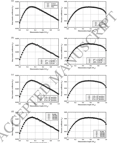
In order to examine the effect of the grid resolution on the wall heat transfer and pressure coefficients, a set of simulations using standard, fine, and coarse

meshes were performed. Grid independence was investigated by performing

105

calculations for different numbers of cells in the x- and y-directions, and then comparing with a solution calculated on the standard grid. Figure 1 shows the standard computational domain which was divided into two regions. Region 1 consists of 10 cells along side I-B and 80 cells along side II, while region 2 consists of 200 cells distributed along side I-A and 80 cells normal to the plate

110

surface, i.e., along side IV. In this way, the effect of altering the cell size in the

x-direction may be analyzed for coarse and fine grids by halving or doubling the number of cells with respect to the standard grid, while the number of cells in the y-direction is kept constant. The same procedure is adopted for the

y- direction, i.e., the cell size is altered keeping the number of cells in thex

-115

direction constant. According to Figure 2(a), the grid sensitivity analysis shows

good agreement for the three mesh sizes investigated indicating that the results were essentially grid-independent.

In a similar manner to the grid independence study, the influence of the time step size on the aerodynamic properties was examined. The time step is chosen

120

to be smaller than both the mean collision time (MCT) and the cell residence time (∆tres), with the latter being the time taken by a DSMC particle to cross a

(7)

ACCEPTED MANUSCRIPT

the reference time step (∆tref) was set to be 6.28× 10−8 s. Then, two time

steps different from the ∆tref were investigated (∆tref)/4 and ( ∆tref)×4. As

125

shown in Fig. 2(b), the resulting simulations are essentially independent of the time step size, so long as the time step and cell size requirements are respected, in conjunction with the other good DSMC practice conditions described above. In DSMC simulations the intermolecular collisions are the principal driver in the flow-field development. These intermolecular collisions occur in each

130

cell, and sufficient particles should be employed not only to reduce the sta-tistical error during the sampling process, but also to ensure the accuracy of the simulated collision rate. However, the use of a large number of particles greatly increases the computational effort. The balance between computational expense and accuracy has been studied by many authors [20–23], and 30-40

par-135

ticles per cell is commonly employed [24–28]. However, there are some DSMC

simulations [29, 30] that employed as few as 10 particles per cell, and some com-putations [31] as many as 50 to 120. The number of particles required is heavily influenced by the choice of collision model, and it is well- known that the majo-rant frequency scheme can use fewer particles than the no time-counter-method

140

(NTC). Recent work has focused on reducing the number of particles required even further [32] using novel collision partner selection schemes. dsmcF oam

uses the NTC method, so requires a reasonably large number of particles in order to recover the collision statistics.

In order to clarify this issue, we executed an additional study to consider

145

the influence of the number of simulated particles on thedsmcFoam solution of a hypersonic flow over a flat plate. Considering that the standard mesh corre-sponded to a total of 43.7 million particles (or 13 particles per cell on average),

two new cases were investigated using the same mesh. These cases corresponded, on average, to 21.8 and 87.4 million particles in the entire computational

do-150

main. The effects of such variations on the heat transfer and pressure are shown in Fig. 2( c). According to these results, the standard grid with a total of 43.7 million particles is considered sufficient for the present computations.

(8)

ACCEPTED MANUSCRIPT

of time steps that results are sampled over (Ns) [24–30]. Since the macroscopic

155

properties of the flow are obtained by sampling all particles within a cell, the number of samples must be sufficient to minimize the statistical error. The magnitude of the statistical error reduces with the square root of the sample size, and it is important to determine the value of Ns that provides acceptable

data scattering. For this purpose, the standard grid with approximately 43.7

160

million particles was run for 50,000, 100,000, 200,000, and 300,000 sampling

time steps. Figure 2(d) shows very good agreement across the range of number of samples considered. Based on these plots, an Ns of 300,000 was considered

as providing an acceptable fluctuation level for the case investigated.

In this section, hypersonic non-reacting gas flow simulations over a zero

165

thickness flat plate were performed. Grid spacing, time step size, number of particles per cell, and number of computational samples were examined in

or-der to test that the assumptions adopted as standard would lead to results independent of the grid, time step and number of statistical samples. On ex-amining these results, no appreciable changes were observed; however, altering

170

the parameters mentioned above, significantly impacted on the computational efficiency of the simulations. In the next section, we adopted the standard pro-cedure for all of the simulations, and the results obtained usingdsmcF oamare

(9)

ACCEPTED MANUSCRIPT

0.010 0.015 0.020 0.025 0.030

0.0 0.2 0.4 0.6 0.8 1.0

H eat tr an sfe r coe ffi ci en t (C h )

Dimensionless length (X/Lp)

Coarse Standard Fine (a) 0.00 0.02 0.04 0.06 0.08

0.0 0.2 0.4 0.6 0.8 1.0

Pressure coefficient (C

p

)

Coarse Standard Fine 0.010 0.015 0.020 0.025 0.030

0.0 0.2 0.4 0.6 0.8 1.0

Dimensionless length (X/Lp) ∆t/4 = 1.57x10-8s ∆t_ref= 6.28x10-8_s ∆tx4 = 2.51x10-7s (b) 0.00 0.02 0.04 0.06 0.08

0.0 0.2 0.4 0.6 0.8 1.0

p

)

Dimensionless length (X/Lp) ∆t/4 = 1.57x10-8_s ∆tref = 6.28x10-8 s ∆tx4 = 2.51x10-7 s

0.010 0.015 0.020 0.025 0.030

0.0 0.2 0.4 0.6 0.8 1.0

Dimensionless length (X/L_p) 2.18 x 107particles 4.37 x 107particles 8.74 x 107particles

(c) 0.00 0.02 0.04 0.06 0.08

0.0 0.2 0.4 0.6 0.8 1.0

p

)

2.18 x 107_particles

4.37 x 107 particles 8.74 x 107 particles

0.010 0.015 0.020 0.025 0.030

0.0 0.2 0.4 0.6 0.8 1.0

Dimensionless length (X/L_p) 50,000 100,000 200,000 300,000 (d) 0.00 0.02 0.04 0.06 0.08

0.0 0.2 0.4 0.6 0.8 1.0

p

)

50,000 100,000 200,000 300,000

Figure 2: (a) Effect of varying the number of cells, (b) the time step, (c) the number of

samples, and (d) number of DSMC particles per cell on the heat transfer (left column) and

[image:9.595.82.487.158.652.2]

(10)

ACCEPTED MANUSCRIPT

4. Benchmark test cases for dsmcFoam

175

The validation strategy consists of comparing the results obtained using

dsmcFoam with other numerical, analytical, or experimental results available in

the literature. In the following sections, the validation process fordsmcFoam is discussed in detail.

4.1. Benchmark Case A: Flow over sharp and truncated flat plates

180

Rarefied hypersonic flow over flat plates has been studied theoretically,

ex-perimentally, and numerically by many authors, e.g., [33–40]. The extremely simple geometry makes the flat plate one of the most useful test cases for nu-merical validation purposes.

The test cases we choose to validatedsmcFoam for non-reacting flows are

185

based on the experimental-numerical study conducted by Lengrandet al. [19] and All`egre textitet al. [37]. In their experimental work, sharp and truncated

flat plates of 0.1 m length (Lp), 0.1 m width (Wp), and 0.005 m thick (Tp) were

positioned in a flow of nitrogen at two angles of incidence, 0◦ and 10◦. The physical model was supplied with an internal water cooling system which

main-190

tained the wall temperature at 290 K. Wall pressure and heat flux measurements were made by placing pressure transducers and chromel-alumel (Ch/Al) ther-mocouples along the longitudinal symmetry axis of the flat plates. In addition, density flowfield measurements were carried out by employing an electron beam

fluorescent technique. The uncertainties in the experimental pressure, heat flux

195

and density measurements were estimated to be 15

In addition to the experimental work, numerical simulations were performed using the NSF equations [19, 37] and the DSMC method [19, 37, 39]. The NSF results were obtained at ONERA using an implicit finite-volume method taking into account velocity slip and temperature jump at the wall. The DSMC

in-200

(11)

ACCEPTED MANUSCRIPT

by Lengrand et al. [19], vibrational molecular energy was neglected and the

Larsen-Borgnakke model [41] was employed for rotational-translational energy

205

exchange. Particle collisions and collision sampling were performed using the variable hard sphere (VHS) model and the time-counter technique (TC) [9], re-spectively. However, the diatomic molecular collision (DMC) model [42] and the null-collision technique (NCT) [43] were adopted by Tsuboiet al.[39]. Since the data and assumptions employed in each method are available in the literature,

210

the discussions below are limited only to details considered necessary.

In order to validate dsmcFoam, 3D sharp and truncated flat plates, as il-lustrated in Fig. 3, with the same dimensions as in Lengrand et al. [19] and All`egre et al. [37], were modeled. In the present computational solution, the two plates were immersed in nitrogen gas with an inlet imposed 0.005 m

up-215

stream of the plate. The freestream conditions (Table 1) and the computational

domains are similar to those presented in Section 3. The computational mesh was composed of 4.7 million and 3.4 million cells for the sharp and truncated cases, respectively. On average, 13 DSMC particles per cell were employed in the simulations; the VHS collision model was applied, and the energy exchange

220

between the translational and rotational modes was modeled using the Larsen-Borgnakke algorithm [41]. The NTC [44] technique was used to control the

molecular collision sampling. The value of rotational collision number (Zrot)

was set to be 1 for the sharp plate to match that used by Lengrandet al. [19]. No information forZrot in the truncated flat-plate case was given by All`egreet

225

al.[37], therefore we used Zrot= 1 andZrot= 5 to compare with their results.

Additional simulation parameters are given in Table 2.

The resulting normalized density (ρ/ρ_∞) contours for zero-thickness, sharp,

and truncated flat plates are shown in Fig. 4, compared with other numerical and experimental results. Despite the different energy redistribution models

230

(12)

ACCEPTED MANUSCRIPT

(a)

x

IV

I-A y

M∞

III

Lp

H II

Sharp flat plate

IV III

(b)

x

IV

I-A y

M∞

I-B

III

Lp

H II

Truncated flat plate

Bevel angle = 20 deg. Thickness = 5 mm

Flat plate length (Lp) = 0.1 m Flat plate width (Lw) = 0.1 m

Figure 3: 2D schematic of sharp (a) and truncated (b) flat plates.

Table 2: Numerical parameters for the flat-plate simulations.

Parameters Zrot ω dref [m] ∆t[s] M CT [s] λ∞[m]

Sharp 1 0.74 4.17×10−10 _6.28_×₁₀−8 _1.90_×₁₀−5 _3.35_×₁₀−3

(13)

ACCEPTED MANUSCRIPT

0.0 1.0 0.0 1.0 X/Lp Y/H 0.7 0.8 0.9 1.2 1.3 1.5 1.6 1.0 1.1 1.4 0.7 1.1

DSMC [Tsuboi et al.]

dsmcFoam 0.8 0.9 1.2 1.3 1.5 1.6 1.0 1.1 1.4 0.7

1.1 0.9 0.8

1.2 1.3 1.5 1.0 1.1 1.4 0.7 1.1 1.6 0.8 0.9 1.2 1.3 1.5 1.6 1.0 1.1 1.4 0.7

1.1 0.9 0.8

1.2 1.3 1.5 1.6 1.0 1.1 1.4 0.7

1.1 0.9 0.8

1.2 1.3 1.5 1.0 1.1 1.4 0.7 1.1 1.6 0.5 1.0

0.0 0.25 0.5 0.75

0.0 1.0 0.0 1.0 X/Lp Y/H 0.7 0.8 0.9 1.2 1.3 1.5 1.6 1.0 1.1 1.4 0.7 1.1

DSMC [Tsuboi et al.]

dsmcFoam 0.8 0.9 1.2 1.3 1.5 1.6 1.0 1.1 1.4 0.7

1.1 0.9 0.8

1.2 1.3 1.5 1.0 1.1 1.4 0.7 1.1 1.6 -0.9 0.8 0.9 1.2 1.3 1.5 1.6 1.0 1.1 1.4 0.7 1.1 0.5

0.0 0.25 0.5 0.75 1.0

1.0

X/Lp Y/H

0.7

Experiments [Allègre et al.]

dsmcFoam symmetry line 1.0 0.0 - 0.2 1.7 1.7 1.8 1.8 1.9 1.9 2.0 0.7 0.8 0.9 1.0 1.1 1.2 1.3 1.4 1.5 1.6 1.1 1.2

1.3 1.41.5

1.6

2.2 2.1 2.0

0.0

X/Lp 1.0

0.0

Figure 4: Density ratio (ρ/ρ∞) contours around zero thickness (top left), sharp (top right),

(14)

ACCEPTED MANUSCRIPT

The normalized density (ρ/ρ_∞) and temperature (T/T_∞) distributions

nor-mal to the sharp flat-plate surface at the non-dimensional streamwise location

235

X/Lp= 0.75 are shown in Fig. 5. Good agreement is found between the DSMC

calculation and the experimental results. The density peak is captured well by the present simulation, and the normalized density profile follows the same trend of the numerical and experimental results performed by Tsuboiet al.[39] and Lengrandet al.[19], respectively. The NSF simulations of Lengrandet al.[19]

240

were not able to predict correctly the density profile at the position considered. Analyzing the translational and rotational temperature profiles in Fig. 5(b), a difference between the rotational and translational temperatures is observed, which indicates thermally non-equilibrium conditions. The normalized tem-perature is low close to the surface, increases to a maximum value inside the

245

shock layer at Y = 0.05 and then declines to the freestream temperature at the

upper boundary condition. In general, there is very close agreement of trans-lational and rotational temperature profiles from dsmcFoam and the CNRS DSMC code [19].

0.0 0.2 0.4 0.6 0.8 1.0 1.2

0.6 0.8 1.0 1.2 1.4 1.6 1.8 2.0

Dimensionless height (Y)

Density ratio (ρ/ρ∞)

X/Lp = 0.75

dsmcFoam DSMC [Tsuboi et al.] DSMC [Lengrand et al.] Exp. [Lengrand et al.] N-S [Lengrand et al.]

(a)

0.0 0.2 0.4 0.6 0.8 1.0

0 10 20 30 40 50

Temperature ratio (T/T∞) X/Lp = 0.75

Empty symbols - dsmcFoam Full symbols - DSMC [Lengrand et al.]

Ttra

Trot

(b)

Figure 5: (a) Normalized density (ρ/ρ∞) and (b) normalized temperature (T/T∞) profiles

(15)

ACCEPTED MANUSCRIPT

Figure 6 shows the heat transfer (Ch), pressure (Cp) and skin friction (Cf)

250

coefficients along the flat plates. For the sharp flat plate case (left column) the comparison of thedsmcFoam results with the experimental data is better than than found by Lengrand et al. [19] and Tsuboi et al. [39]. The skin friction coefficient shows good agreement with the Lengrand et al. [19] DSMC results at the leading edge and from position X/Lp ∼= 0.4 to 1.0. When the NSF

255

calculations for Chand Cpfor a rarefied flow over a sharp flat plate are compared

with experimental and DSMC results, it is clear that the CNRS NSF simulations were unable to capture the surface quantities for the conditions investigated.

According to Lengrandet al.[19], possible sources of experimental error are related to uncertainties in the freestream conditions, measurement procedures,

260

and the influence of the leading edge bluntness or bevel angle. In order to investigate the impact of the leading edge bluntness, Fig. 6 (right column) shows

comparisons of the dsmcFoam results with experimental data from All`egreet al. [37] and previous DSMC simulations. From the heat transfer (Ch) plot,

excellent agreement is seen between the DSMC simulations apart from at the

265

leading edge (X/Lp = 0) where the dsmcFoam results do not tend to zero.

Both computations demonstrated significant difference when compared with experimental data.

In contrast with Ch results, the pressure coefficient (Cp) shows very good

agreement between numerical and experimental data. However, the numerical

270

results show slightly higher values for Cpat the flat-plate leading edge. For the

skin friction coefficient along the truncated flat plate, no numerical results were available in the literature. Since the value of Zrotwas not specified in Ref. [37],

dsmcFoam computations for rarefied gas flow over the truncated flat plate were

performed with Zrot= 1 and 5; however, no significant differences in the surface

275

quantities were observed.

In summary, hypersonic non-reacting gas flow over three-dimensional zero-thickness, sharp, and truncated flat plates was simulated usingdsmcFoam. Ex-cellent agreement between numerical and experimental data for the density con-tours was found. The results also demonstrated that the shape of the leading

(16)

ACCEPTED MANUSCRIPT

0.015 0.020 0.025 0.030 0.035

0.0 0.2 0.4 0.6 0.8 1.0

Heat transfer coefficient (C

h

)

0.01 0.02 0.03 0.04 0.05 0.06

0.0 0.2 0.4 0.6 0.8 1.0

Heat transfer coefficient (C h )

Dimensionless length (X/L_p) dsmcFoam DSMC [Allegre et al.] Exp. [Allegre et al.]``

0.00 0.02 0.04 0.06 0.08

0.0 0.2 0.4 0.6 0.8 1.0

p

)

0.00 0.05 0.10 0.15 0.20

0.0 0.2 0.4 0.6 0.8 1.0

Pressure

coefficient

(C

p

)

Dimensionless length (X/L_p) dsmcFoam DSMC [Allegre et al.] Exp. [Allegre et al.]``

0.03 0.04 0.05 0.06 0.07 0.08

0.0 0.2 0.4 0.6 0.8 1.0

Skin friction coefficient (C

f

)

dsmcFoam DSMC [Lengrand et al.]

0.00 0.04 0.08 0.12 0.16

0.0 0.2 0.4 0.6 0.8 1.0

Skin friction coefficient (C

f

)

dsmcFoam

Figure 6: Comparisons of heat transfer (Ch), pressure (Cp), and skin friction coefficients (Cf)

fromdsmcFoam simulations and independent numerical/experimental data for sharp ( left)

and truncated (right) flat plates.

edge can affect the flow and shock structure over the plate. For the aerodynamic properties on a sharp flat plate, satisfactory agreement was found from the lead-ing edge up to X/Lp= 0.2; however, certain discrepancies were observed further

along the plate. In contrast, the truncated case exhibited differences between the numerical and experimental data in the leading edge region, while better

(17)

ACCEPTED MANUSCRIPT

agreement was evident towards the trailing edge. Comparisons between the

DSMC and NSF results demonstrate that the continuum approach, even when using slip velocity and temperature jump boundary conditions, cannot be used with confidence to predict these types of thermodynamically non-equilibrium flows.

290

4.2. Benchmark Case B: Flow over a 70◦ blunted cone

The flow over blunt bodies at high speeds and high altitudes displays com-plex flow interactions, and requires a precise determination of the heating rate,

aerodynamic forces, and the flowfield surrounding the body. The characteriza-tion of the wake region is also a key factor for the success of re-entry missions.

295

In an experimental set-up, a 70◦_{blunted cone, identical in geometric}

propor-tions to that of the Mars Pathfinder probe, was chosen by the AGARD Working Group 18 [45]. Rarefied flow experiments were performed in five different facil-ities: the SR3 wind tunnel at CNRS-Meudom, the V2G, V3G and HEG wind

tunnels at DRL-G¨ottingen, and the LENS wind tunnel at the Buffalo Research

300

Center (Calspan, University of Buffalo, USA). The experimental test conditions used in each of these experimental facilities are available in Ref. [45].

All`egre et al. [46–48] provided detailed information regarding experiments conducted at CNRS-Meudon. The CNRS group employed three freestream flow conditions, representative of different levels of rarefaction, and three probe

305

models, each one having a base and afterbody sting diameter of 0.05 and 0.0125 m, respectively.

The CNRS model utilized for the flowfield density measurements was made of brass, water cooled, with a wall temperature remaining close to 290 K during all measurements. An electron beam fluorescent technique was used to

mea-310

sure the density field around the blunted cone [46]. For the aerodynamic force

measurements, the model was made of aluminum, uncooled, with the wall tem-perature estimated to be close to 350 K. The model was directly attached to an external balance providing direct measurements of drag, lift, and pitching moment, and indirect determinations of the center of pressure at different

(18)

ACCEPTED MANUSCRIPT

gles of attack [47]. For heat transfer measurements, a steel model was used

in which the wall temperature was kept close to 300 K [48] . Chrome-alumel (Ch/Al) thermocouples were embedded through the wall thickness at nine lo-cations along the forebody, base plane, and sting, and the thin-wall technique was applied to measure the heat fluxes on the steel probe.

320

An extensive set of simulations at these experimental test conditions were completed using both DSMC [49–58] and Navier-Stokes [59–62] methods prior

to the release of the experimental data. In this way, it was possible to perform a blind validation test of the computational codes.

In the present work, the simulated freestream conditions are the same as

325

those used in the SR3 low-density wind tunnel (case 1) [46–48]. The Mars Pathfinder probe was immersed in a non-reacting uniform nitrogen flow of ve-locity, mass density, and temperature equal to 13.316 m/s, 1.73×10−5 _kg/m3_,

and 13.316 K, respectively. Energy exchange was allowed between the transla-tional and rotatransla-tional modes and was controlled by the Larsen-Borgnakke

phe-330

nomenological model [41]. Molecular collisions were modeled using the variable hard sphere (VHS) model [63], and the no-time-counter (NTC) collision sam-pling technique [44]. In addition, simulation parameters for N2 are: reference

diameter (dref), rotational collision number (Zrot) and viscosity index (ω) set

equal to 4.17×10−10_{m, 5, and 0.74, respectively [9].}

335

Figure 7(a) shows the experimental model configuration and Fig 7(b) gives an amplified view of thedsmcFoamcomputational grid. The computational grid was composed of a mixture of 7.1 million hexa- and polyhedral cells with, on average, 10.5 simulated particles per cell. A uniform hexahedral mesh, with cell sizes smaller than the freestream mean free path, is used for most of the domain,

340

with some polyhedral cells to capture the surface geometry. Each simulation was performed using 240 processors on the parallel machine at the University of Strathclyde, and 10 days were required to fully resolve each of the cases.

The computational domain was large enough so that the upstream, down-stream, and upper boundary conditions could be specified as freestream. In

345

(19)

ACCEPTED MANUSCRIPT

0◦ _{angle of attack. Undisturbed freestream conditions were imposed 0.02 m}

upstream of the probe, and the computational domain normal to the probe ex-tended a distance 0.08 m in they- andz-directions. The surface temperature was set at 290 K, 300 K, and 350 K for the density, heat transfer and aerodynamic

350

force measurements, respectively. The surface boundary condition assumed the gas-surface interaction to be diffuse, with full thermal accommodation at the specified surface temperature.

(a) (b)

Mars Pathfinder Probe

x

y z

9 8 7 6

5 4 3 2 1

Ma

Rn α

Locations S/Rn (Rn - 12.5 mm) Thermocouples

0.00 0.52 1.04 1.56 2.68 3.32 5.06 6.50 7.94

1 2 3 4 5 6 7 8 9

50

45

20

10 0.4

70o 20o

10 35 Rn = 12.5

Rj = 2.08 Rc = 2.08

75

120.4

Figure 7: (a) Experimental 70◦ _{blunted cone model for heat transfer measurements with}

thermocouple locations from [48], and (b) schematic of the corresponding dsmcFoam 3D

computational mesh.

In Fig. 8 experimental density flowfields at different angles of attack [46] are compared with the results from thedsmcFoam calculations. Qualitatively, the

355

results show a good level of agreement between the experimental anddsmcFoam

results. According to All`egre et al.[46] the flowfield density measurement ac-curacy is estimated to be 10%, except in the region encompassing the forward

shock wave, which is characterized by high density gradients and has a higher uncertainty.

360

(20)

simula-ACCEPTED MANUSCRIPT

tions, developed at the NASA Johnson Space Flight Center [64] and available

in Ref. [49]. In Fig. 9, excellent agreement of the density ratio (ρ/ρ∞), overall

temperature (Tov), and Mach number (M) contours at 0◦degree angle of attack

is found between the codes; where

Tov= Ttransξtrans+Trotξrot

ξtrans+ξrot , (2)

with Ttrans and Trot the translational and rotational temperatures of the gas,

respectively, andξtrans andξrotthe number of degrees of freedom in the

(21)

ACCEPTED MANUSCRIPT

0 10 20 30 50 60 70 80 40 Level 1 2 3 4 5 6 7 8 9 A B C D E F G H I J ρ/ρ∞ 0.1 0.2 0.3 0.4 0.5 0.6 0.7 0.8 0.9 1.1 1.3 1.5 1.7 2.0 2.5 3.0 4.0 5.0 6.0 7 5 4 2 3 6 D BA 8 9 C E F G H I J D C B A SR3 experiments dsmcFoam Z [mm]

-20 0 20 40 60 80

α = 0o

0 10 20 30 50 60 70 80 40 Level 1 2 3 4 5 6 7 8 9 A B C D E F G H I J ρ/ρ∞ 0.1 0.2 0.3 0.4 0.5 0.6 0.7 0.8 0.9 1.1 1.3 1.5 1.7 2.0 2.5 3.0 4.0 5.0 6.0 7 5 4 2 3 6 D B A 8 9 C E F G H I J D C B A dsmcFoam Z [mm]

-20 0 20 40 60 80

SR3 experiments α = 10o

0 10 20 30 50 60 70 80 40 Level 1 2 3 4 5 6 7 8 9 A B C D E F G H I ρ/ρ∞ 0.2 0.3 0.4 0.5 0.6 0.7 0.8 0.9 1.1 1.3 1.5 1.7 2.0 2.5 3.0 4.0 5.0 6.0 6 4 4 2 3 5 C A 8 7 B E F G H J B A dsmcFoam Z [mm]

-20 0 20 40 60 80

1

C

9 D

SR3 experiments α = -10o

Figure 8: Density ratio (ρ/ρ∞) distributions from dsmcFoam, and from the SR3

(22)

ACCEPTED MANUSCRIPT

0.00

0.04

0.08

0.12

-0.04 0.00 0.04 0.08 0.12

y [m]

1.5

1.01 1.1

6 4

0.5 0.4

0.6 2

0.3 0.2

0.1 _0.3

0.35 0.35

2 1.01 1.5 1.1

dsmcFoam DAC

0.00

0.04

0.08

0.12

-0.04 0.00 0.04 0.08 0.12

y [m]

400

400 300 200 100 50 500

800 600

DAC

dsmcFoam

0.00

0.04

0.08

0.12

-0.04 0.00 0.04 0.08 0.12

y [m]

1 2 3

4

8 12 1

dsmcFoam DAC

Figure 9: (top left) Density ratio (ρ/ρ∞), (top right) overall temperature (Tov), and (bottom)

Mach number (M) distributions fromdsmcFoam and from the DAC simulations [49] at 0◦

(23)

ACCEPTED MANUSCRIPT

The aerodynamic forces and moments have also been experimentally and

numerically investigated [47, 51, 53] for different angles of attack. In Figs. 10

365

and 11 a satisfactory concurrence is found between the experimental data and

dsmcFoamsimulations. According to All`egreet al.[47], the global uncertainty in the aerodynamic coefficients and forces did not exceed±3%, and the maximum difference between measured and simulated results was 8.6% on the normal force at 30circ _{angle of attack. Table 3 shows the drag and lift coefficients, and the}

370

axial and normal forces coefficients, from the experimental measurements and numerical predictions using thedsmcFoam code.

1.3 1.4 1.5 1.6 1.7 1.8

-5 0 5 10 15 20 25 30 35

Drag coefficient (C

d

)

Angle of attack (α)

SR3 experiments DAC dsmcFoam

-0.4 -0.3 -0.2 -0.1 0.0

-5 0 5 10 15 20 25 30 35

Lift coefficient (C

l

)

Angle of Attack (α)

SR3 experiments dsmcFoam

Figure 10: Drag (Cd) and lift (Cl) coefficients at different angles of attack (α).

1.3 1.4 1.5 1.6 1.7 1.8

-5 0 5 10 15 20 25 30 35

Axial force coefficient (C

A

)

Angle of attack (α)

SR3 experiments dsmcFoam

0.0 0.1 0.2 0.3 0.4 0.5

-5 0 5 10 15 20 25 30 35

Normal force coefficient (C

N

)

Angle of attack (α) SR3 experiments dsmcFoam

(24)

ACCEPTED MANUSCRIPT

Table 3: Experimental anddsmcFoam-calculated aerodynamic and force coefficients.

Angle Drag Lift Axial force Normal force

exp. calc. % diff. exp. calc. % diff. exp. calc. % diff. exp. calc. % diff. 0o _1.657 _1.652 _0.302 _0.000 _0.000 _0.000 _1.657 _1.652 _-0.302 _0.000 _0.000 _0.000

5o _1.629 _1.642 _0.798 _-0.057 _-0.062 _8.772 _1.628 _1.642 _0.860 _0.084 _0.080 _-4.762

10o _1.615 _1.611 _-0.248 _-0.133 _-0.143 _7.519 _1.614 _1.615 _0.0620 _0.148 _0.140 _-5.405

15o _1.569 _1.561 _-0.510 _-0.200 _-0.213 _6.500 _1.568 _1.568 _0.000 _0.213 _0.200 _-6.103

20o _1.538 _1.496 _-2.731 _-0.249 _-0.269 _8.032 _1.530 _1.504 _-1.700 _0.291 _0.266 _-8.591

30o _1.432 _1.350 _-5.726 _-0.324 _-0.351 _8.333 _1.402 _1.344 _-4.137 _0.434 _0.398 _-8.294

The effect of the angle of attack on the heat transfer (Ch) and pressure (Cp)

coefficients is shown in Figs. 12 and 13. In this set of plots, the results are presented as a function of the normalized arc distance (s/Rn) measured from

375

the forebody stagnation point to the end of the sting. Here, the dsmcF oam

results are compared with DSMC computations provided from the DAC [50]

and molecular gas dynamics simulator (MGDS) [40] codes, as well as with the experiments performed at the CNRS facilities [48].

According to Fig. 12, dsmcF oam shows a good agreement with DAC and

380

MGDS for all angles of attack considered. The heat transfer coefficient is cap-tured well by the numerical codes at the forebody and sting regions; however, a significant difference in Chis seen between computations and experiments at

the probe shoulder (S/Rn≈2). This difference is even higher when the angle of

attack is increased, as shown in Fig. 14. At 30◦angle of attack, the flow is

com-385

pressed against the probe shoulder generating high heating rates in this region. Nevertheless, there is no thermocouple at this position; the last thermocouple on the forebody region is located at S/Rn= 1.56 but the simulated heat transfer

peak occurs at S/Rn ≈= 2.0. For this reason, the peak in the heat transfer is

not captured by the CNRS experiments. Even at locations where

thermocou-390

ples are present, both dsmcF oam and MGDS predict higher heat fluxes than the experiments. Again, at 30◦_{angle of attack, MGDS predicts a slightly lower}

heat flux at the stagnation point, compared todsmcF oam. MGDS used a mesh refinement algorithm to ensure cells stay smaller than the local mean free path, whereasdsmcF oamuses a fixed grid, so the cells in the high density region near

(25)

ACCEPTED MANUSCRIPT

the stagnation point may be larger than the local mean free path.

0.0 0.1 0.2 0.3 0.4

0 2 4 6 8 10 12 14

h

)

S/Rn

α = 0°

dsmcFoam DAC MGDS SR3 experiments

0.0 0.1 0.2 0.3 0.4

0 2 4 6 8 10 12 14

h

)

S/Rn

α = 10°

dsmcFoam MGDS SR3 experiments

0.0 0.1 0.2 0.3 0.4

0 2 4 6 8 10 12 14

h

)

S/Rn

α = 20°

dsmcFoam SR3 experiments

0.0 0.1 0.2 0.3 0.4 0.5

0 2 4 6 8 10 12 14

h

)

S/Rn

α = 30°

dsmcFoam MGDS SR3 experiments

Figure 12: Heat transfer coefficients (Ch) along the Mars Pathfinder surface fromdsmcFoam,

DAC, MGDS and CNRS experiments at different angles of attack (α).

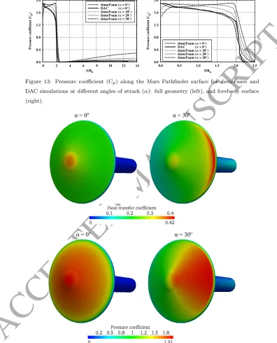
Figure 13 shows the pressure coefficient along the Mars Pathfinder probe surface. Excellent agreement is found between thedsmcF oamand DAC codes for 0◦_{angle of attack. As the angle of attack is increased, the pressure coefficient}

increases at the probe shoulder, following the same trend as the heat transfer

400

(26)

ACCEPTED MANUSCRIPT

0.0 0.4 0.8 1.2 1.6 2.0

0 2 4 6 8 10 12 14

p

)

S/Rn

dsmcFoam (α = 0°) DAC (α = 0°) dsmcFoam (α = 10°) dsmcFoam (α = 20°) dsmcFoam (α = 30°)

0.0 0.4 0.8 1.2 1.6 2.0

0.0 0.5 1.0 1.5 2.0 2.5

p

)

S/Rn

dsmcFoam (α = 0°) DAC (α = 0°) dsmcFoam (α = 10°) dsmcFoam (α = 20°) dsmcFoam (α = 30°)

Figure 13: Pressure coefficient (Cp) along the Mars Pathfinder surface fordsmcFoam and

DAC simulations at different angles of attack (α): full geometry (left), and forebody surface (right).

α = 0o _{α = 30}o

Figure 14: (top) Heat transfer (Ch) and (bottom) pressure (Cp) coefficient contours at 0o

[image:26.595.82.478.163.653.2]

(27)

ACCEPTED MANUSCRIPT

When a probe enters a planetary atmosphere at high velocities, the

fore-body flowfield is dominated by a strong shock wave that causes the excita-tion, dissociation and possibly ionization of the gas surrounding the vehicle. This highly thermochemically non-equilibrium flow rapidly expands around the

405

probe shoulder into the near wake region with a significant increase in rarefac-tion [49, 58, 65]. The flowfield complexity for the Mars Pathfinder probe is shown in Fig. 15(a). Due to this complexity, the aerothermodynamics of the

wake may not be measured accurately; according to Wright and Milos [66] the uncertainty in the aeroheating measurements in this region is typically assumed

410

to be in the range of 50-300%. This level of uncertainty plays a significant role in the vehicle design and the correct selection of a thermal protection system (TPS).

In order to compare the results obtained using the dsmcFoam code with

those from DAC simulations provided by Moss et al. [49], normalised density,

415

velocity, and temperature profiles are presented at four different locations in the probe afterbody region as depicted in Fig. 15(b).

(a) (b)

Diffuse shock

wave Separation of thick

boundary layer

Rapid expansion and freezing: high vibrational temp; low T, p and ρ

Weak shock and recompression

Recirculating flow: possibly unsteady

Shear layer: steep gradients of U, T and ρ

Wake closure: possibly subsonic

X1 = 0.0095 X2 = 0.015 X3 = 0.03 X4 = 0.06

Figure 15: (a) Schematic of the planetary probe flow structure [58], and (b) macroscopic

properties measurement locations.

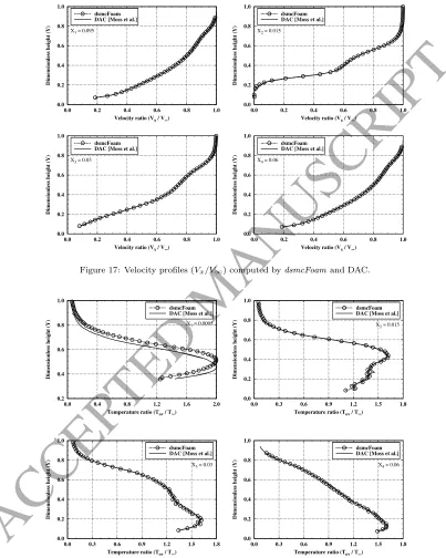
From Figs. 16 to 18, it is clear that there is very good agreement between the DAC and dsmcF oam simulations. However, for the density and temperature profiles at location X1 = 0.0095, some slight discordance is observed. In this

420

(28)

ACCEPTED MANUSCRIPT

between the two simulations may have some influence on the flowfield structure.

0.02 0.03 0.04 0.05 0.06 0.07

0.5 1.0 1.5 2.0 2.5 3.0 3.5 4.0

X1 = 0.0095

dsmcFoam DAC [Moss et al.]

0.0 0.2 0.4 0.6 0.8 1.0

0.0 0.4 0.8 1.2 1.6 2.0 2.4 2.8

X2 = 0.015

0.0 0.2 0.4 0.6 0.8 1.0

0.0 0.4 0.8 1.2 1.6 2.0 2.4 2.8

X3 = 0.03

0.0 0.2 0.4 0.6 0.8 1.0

0.0 0.4 0.8 1.2 1.6 2.0 2.4 2.8

X4 = 0.06

Figure 16: Density profiles (ρ/ρ∞) computed bydsmcFoamand DAC.

To summarize this section, simulations have been performed using the

dsm-cFoamcode for non-reacting flows over both flat plates and the Mars Pathfinder

probe. The present data are compared with experimental and numerical

solu-425

tions available in the open literature. Assuming the average uncertainty in the experimental data to be approximately 10% [19, 37, 46–48], a satisfactory level

(29)

ACCEPTED MANUSCRIPT

0.0 0.2 0.4 0.6 0.8 1.0

Velocity ratio (Vx / V∞) X1 = 0.095

0.0 0.2 0.4 0.6 0.8 1.0

Figure 17: Velocity profiles (Vx/V∞) computed bydsmcFoamand DAC.

0.2 0.4 0.6 0.8 1.0

0.0 0.4 0.8 1.2 1.6 2.0

Temperature ratio (Tov / T∞) X1 = 0.0095

0.0 0.2 0.4 0.6 0.8 1.0

0.0 0.3 0.6 0.9 1.2 1.5 1.8

0.0 0.2 0.4 0.6 0.8 1.0

0.0 0.3 0.6 0.9 1.2 1.5 1.8

0.0 0.2 0.4 0.6 0.8 1.0

0.0 0.3 0.6 0.9 1.2 1.5 1.8

[image:29.595.82.485.159.663.2]

(30)

ACCEPTED MANUSCRIPT

4.3. Benchmark Case C: flow in patterned 2D microchannels

The previous test cases have been for hypersonic flows, but progress has also

430

been made in the extension of thedsmcFoam code to subsonic, pressure-driven flows in micro- or nano-scale geometries. In contrast to the previous cases where the Knudsen number is high because the gas density is low, micro-scale devices

often operate in standard atmospheric conditions. The Knudsen number is high in these types of problems because the characteristic length scaleLis small.

435

dsmcFoam has previously been benchmarked for planar Poiseuille flow with

defined pressure inlets and outlets [67], where comparison to analytical solu-tions for the non-linear pressure profile were presented. The general starting point for the treatment of an inlet or outlet boundary condition in DSMC is

to impose a particle flux. The rate of particle insertion, ˙N, can be computed

440

from the equilibrium Maxwell-Boltzmann distribution, which requires bound-ary values of temperature, density, and velocity. The streaming velocity profiles for internal micro-scale flows at the inlet and outlet boundaries are generally not known a priori, so the boundary conditions described below use the the-ory of characteristics to calculate the local streaming velocity as the simulation

445

proceeds.

Wang and Li [18] proposed an inlet boundary condition with target gas prop-erties of pressure pin and temperatureTin, prescribed at the inflow boundary.

The perfect gas law is used to calculate the inlet number densitynin,

nin= pin

kBTin. (3)

Based on the theory of characteristics, the stream-wiseuinand tangentialvin

ve-locities at two-dimensional inlet boundary facesf, using values from the bound-ary cell centresj, are calculated as

(uin)f =uj+pin−pj

ρjaj , (4)

and

(31)

ACCEPTED MANUSCRIPT

where uj and vj are first order extrapolations from the cells attached to the

relevant boundary face, ρ is mass density and a is the local speed of sound. The pressure pj is calculated in these boundary conditions from the overall

temperature as:

pj =ρjR

3Ttr+ ¯ζrotTrot

3 + ¯ζrot

j

. (6)

At the exit boundaries, only the pressure is defined and the boundary con-ditions are those first proposed by Nanceet al.[68]:

(ρout)f =ρj+pout−pj

(aj)2

, (7)

(uout)f =uj+pj−pout

ρjaj , (8)

(vout)f=vj, (9)

(Tout)f=pout/

h

R(ρout)f

i

. (10)

The pressurepj is again calculated from Eq. (6). The process for selecting the

required translational and rotational energies for particles at the boundaries is standard in DSMC, and details can be found in Ref. [9].

Here, we investigate a pressure-driven flow through a micro-channel with two

450

heated steps on its lower surface, as shown in Fig. 19, which was first considered using DSMC by Fang and Liou [69]. The inlet pressure is 0.73 atm and the inlet

temperature is 300 K, giving an inlet Knudsen number, based on the channel heightHand the VHS mean free path, of around 0.08. Cases with inlet-to-outlet pressure ratios (pin/pout) of 2.5 (Case 1) and 4 (Case 2) are investigated here,

455

using the inlet and outlet boundary algorithms described above. All surfaces are considered to be fully diffuse, with temperatures of 323 K and 523 K forT1and

T2, respectively. The non-uniform, non-isothermal geometry greatly increases

(32)

ACCEPTED MANUSCRIPT

T1

T1 T1

T2 T2

H

h

pout pin

Tin

x y

Figure 19: 2D schematic of the patterned microchannel with different wall temperatures. Dashed lines are measurement locations.

The channel height H is 0.9 µm and the aspect ratio is 6.7. The steps

460

inside the channel have a height h of 0.3 µm, a length of 1.0287µm, and re-spective leading edge positions of 1. 4787 µm and 3.4713 µm. The working gas is nitrogen, with standard VHS parameters ofω= 0.77 anddref = 4.17×

10−10 _{m at a reference temperature of 273 K, and Larsen- Borgnakke energy}

exchange performed on a ‘single molecule’ basis, where each collision partner is

465

considered in turn for relaxation with a constant rotational relaxation number of 5. Vibrational energy is excluded from the calculations because of the rel-atively low temperatures involved. Many of these parameters are not defined in Fang and Liou [69], so there may be some uncertainty in the results. 7656 rectangular computational cells, and a constant time step of 1× 10−11 _{s were}

470

used in thedsmcFoamsimulations; post-processing of the results confirmed that these parameters met good DSMC practice throughout the entire domain. The

dsmcFoam results that follow have been sampled for 200,000 time steps after

steady state was achieved. Case 1 comprised around 220,000 DSMC particles, and Case 2 had 300,000. The simulations were performed in parallel on two

475

cores of a desktop PC equipped with an i7 processor, and took around 24 hours

for each simulation. Figure 20 shows the contours of overall temperatureTov

for Case 2.

Figure 21 shows a comparison of the overall temperature profiles for the

pin/pout = 2.5 case, along two lines for the length of the channel. These two

480

locations are illustrated by the dashed lines in Fig. 19; the first location is at the top of the steps, while the second one is mid-way between the top of the steps and

(33)

ACCEPTED MANUSCRIPT

Figure 20: Contours of constant overall temperature, forpin/pout= 4.

can be seen here, with the peaks in the temperature profiles corresponding to the locations of the steps. The results for Case 2 also show excellent agreement,

485

but have been omitted for conciseness.

300 320 340 360 380 400 420 440 460 480

0 1 2 3 4 5 6

Tov

(K)

x/h

Step - Fang & Liou (2002) Top-Mid - Fang & Liou (2002) Step - dsmcFoam

Top-Mid - dsmcFoam

Figure 21: Comparison of temperature distribution results from from Fang and Liou [69], and

dsmcFoamforpin/pout= 2.5.

Figure 22 shows the heat transfer at the upper surface for bothpin/pout= 2.5

and 4. In general, the agreement between the DSMC results is very good, but

dsmcFoampredicts a slightly higher heat transfer fromx/h= 2.4 to 3.4 for both

pressure ratios. The peak heat transfer around the step locations are lower for

490

(34)

ACCEPTED MANUSCRIPT

rarefied and so heat transfer from the gas to the surface is reduced.

-1 0 1 2 3 4

0 1 2 3 4 5 6

q

(

×

10

6 J/

s)

x/h

Case 1 - Fang & Liou (2002) Case 2 - Fang & Liou (2002)

Case 1 -dsmcFoam

Case 2 -dsmcFoam

.

Figure 22: Comparison of the results for heat transfer at the upper surface from Fang and

Liou [69] anddsmcFoam.

4.4. Benchmark Case D: Knudsen minimum

In order to compare micro-scale results fromdsmcFoam to available experi-mental data, a series of 2D isothermal pressure-driven Poiseuille flows of nitrogen

495

gas are solved over a large range of Knudsen number. Figure 23 is a sketch of the simple geometry.

p

_out

h

L

p

_in

T

_in

Figure 23: 2D micro-channel geometry for pressure-driven Poiseuille flow.

The variable hard sphere collision model is used with the standard nitrogen

properties at a reference temperature of 273 K, i.e. viscosity coefficientω= 0.74 and reference diameterdref = 4.17 ×10−10 m. The mass flux ˙mis measured

(35)

ACCEPTED MANUSCRIPT

and normalized as follows:

Q= mL˙

√

2RT

h(pin−pout), (11)

where L and h are the length and height of the 2D planar Poiseuille flow channel, respectively, and R is the specific gas constant; T is the isothermal temperature that the simulations were performed at, which is 273 K. This value is used for the boundary condition of the inlet gas temperature, and is also

505

the temperature assigned to the fully diffuse surfaces of the channel walls. The

inlet pressurepinand outlet pressurepoutare set using the boundary conditions

procedure of§4.3. A rarefaction parameterδmis defined as the averageKnm of

the inlet and outlet Knudsen numbers (based on the VHS mean free path and the channel heighth) in each case:

510

δm=

√

π

2Knm

. (12)

1.2 1.6 2 2.4 2.8 3.2

0.01 0.1 1 10

Q

δm

dsmcFoam

Karniadakis (2005) Ewart et al. (2007)

Figure 24: Normalised mass flow rate, showing the Knudsen minimum phenomenon.

(36)

ACCEPTED MANUSCRIPT

previous DSMC results [70] using nitrogen gas in a channel of the same aspect

ratio. Experimental results from Ewart et al. [71], which were obtained with

515

helium gas, are also plotted for comparison. The two sets of DSMC results are in good agreement, and the agreement with experimental data is excel-lent at lowKn and reasonable at high Kn. It has previously been noted [72] that the asymptotic value thatQ obtains is proportional to ln (L/h); since the experimental work was performed on geometries with very large aspect ratio

520

(L/h= 1000), it is expected that the DSMC results for an aspect ratio of 20 will not match exactly. Unfortunately, it is not possible to simulate an aspect ratio of 1000 using DSMC, as the velocities would be too low to obtain a con-verged solution in a practical time scale. The famous Knudsen minimum [73] can clearly be observed in Fig. 24, where the normalized mass flow rate has a

525

minimum at aboutKn = 1.

5. Conclusions

The verification and validation of new developments and features in the

dsmcF oamcode have been presented for high and speed non-reacting flows in different geometries. First, sensitivity analyses were carried out for mesh, time

530

step, number of samples and particles was carried out for a flow over a zero-thickness flat plate. Choosing cell sizes, time steps, number of particles, and number of samples withing the ranges dictated by good DSMC practice, led to solutions that were independent of these simulation parameters.

The validation procedure aimed to compare computed dsmcF oam results

535

with other numerical and experimental data available in the literature. Four

different geometries were employed in the investigation: sharp and truncated flat plates, the Mars Pathfinder probe, a micro-channel with heated steps, and a simple micro-channel. In the flat plate cases, the density contours and temper-ature profiles showed a good concurrence between numerical and experimental

540

(37)

ACCEPTED MANUSCRIPT

edges of the sharp and truncated flat plates, respectively. In addition,

conven-tional CFD results showed marked differences from both the DSMC simulations and experimental data, demonstrating that rarefied gas effects are not captured

545

well by a continuum-based solver.

Hypersonic rarefied non-reacting gas flows over the Mars Pathfinder probe were also investigated. ThedsmcF oamsolver demonstrated its capabilities to successfully resolve hypersonic flows over such complex geometries.

Aerody-namic surface quantities, the flow structure in the shock and wake regions, the

550

drag, lift, and axial and normal forces acting on the probe all show a high level of agreement with CNRS experiments as well as numerical results from the DAC and MGDS codes.

In addition to the high speed benchmark cases, low speed gas flow through a micro-channel with two heated steps was considered in order to further validate

555

the new pressure-driven dsmcF oam boundary conditions. The results were compared with published DSMC simulations, and an excellent level of agreement was found. In order also to compare with available micro-scale experimental data, normalized mass fluxes were calculated over a range of Knudsen numbers to demonstrate that the Knudsen minimum in Poiseuille channel flow can be

560

captured. The results of these cases further validates the work reported in

Refs. [15, 67] on subsonic, prescribed pressure inlets and outlets.

6. Acknowledgements

The authors acknowledge the financial support provided by Conselho Na-cional de Desenvolvimento Cient´ıfico e Tecnol´ogico (CNPq/Brazil) under Grant

565

(38)

ACCEPTED MANUSCRIPT

References

[1] P. J. Roache, Need for control of numerical accuracy, Journal of Spacecraft

570

and Rockets 27 (2) (1990) 98–102.

[2] G. Sheng, M. S. Elzas, T. I. Oren, Cronhjort, Model validation: a systemic and systematic approach, Reliability Engineering ans System Safety 42 (1993) 247–259.

[3] P. J. Roache, Verification of codes and calculations, AIAA Journal 36 (5)

575

(1998) 696–702.

[4] P. J. Roache, Verification and validation in computational science and en-gineering, Hermosa Publishers, Albuquerque, NM, 1998.

[5] American Institute of Aeronautics & Astronautics Staff, AIAA guide for the verification and validation of computational fluid dynamics simulations.,

580

American Institute of Aeronautics and Astronautics, 1998.

[6] W. L. Oberkampf, T. G. Trucano, Verification and validation in computa-tional fluid dynamics, Progress in Aerospace Sciences 38 (SAND2002-0529) (2002) 209–272.

[7] W. L. Oberkampf, T. G. Trucano, C. H. Hirsch, Verification, validation,

585

and predictive capabilities in computational engineering and physics, Tech. Rep. 2003-3769, Sandia National Laboratories (2003).

[8] W. L. Oberkampf, M. F. Barone, Measures of agreement between

computa-tion and experiment: validacomputa-tion metrics, Journal of Computacomputa-tional Physics 217 (2006) 5–36.

590

[9] G. Bird, Molecular Gas Dynamics and the Direct Simulation of Gas Flows,

Clarendon, Oxford, 1994.

[10] I. D. Boyd, G. Chen, G. V. Candler, Predicting failure of the continuum fluid equations in transitional hypersonic flows, Physics of Fluids 7 (1) (1995) 210–219.