Wave Parameter Hindcasting in
a Lake Using the SWAN Model
M.H. Moeini
1and A. Etemad-Shahidi
1;Abstract. Wind-induced wave characteristics are one of the most important factors in the design of coastal and marine structures. Therefore, accurate estimation of wave parameters is of considerable importance. The wave climate study can be conducted by eld measurements, empirical studies, physical modeling and numerical simulations. In this paper, the skill of a third-generation spectral model called SWAN has been evaluated in the prediction of wave parameters. The varying wind and wave climate of Lake Erie in the year 2002 has been used for evaluation of the model. The signicant wave height (Hs)
and the peak spectral wave period (Tp) were the parameters employed in the study and the model has
been executed in a nonstationary mode. The linear and exponential growth from wind input, four-wave nonlinear interaction, whitecapping and bottom friction have been considered in the simulation. The results of this study show that in the investigated case, the average scatter index of SWAN is about 19 percent for signicant wave height and 23 percent for the peak period. The error of the SWAN model in prediction of the wave height and period reduced about 3 percent after elimination of wave heights less than 0.5 meters. It was also found that using the cumulative steepness method for whitecapping dissipation yields worse results for signicant wave height and better results for peak spectral period estimation. After using this method, the average scatter index for the prediction of Hs increased about 5 percent and decreased more
than 4 percent for Tp. It should be mentioned that the computational time required by using this method
is approximately more than twice that of the Komen option.
Keywords: Wave prediction; Numerical model; Third generation; Lake Erie.
INTRODUCTION
In the marine environment, the planning of sustainable development of economic activities requires long term information about environmental conditions such as waves. Accordingly, the knowledge of wind wave statistical characteristics is necessary in a variety of applications including the design of coastal structures, studies of sediment transport, coastal erosion and pollution processes. Due to the lack of such information in many regions, the wave characteristics are estimated using dierent methods. Generally, wave climate sim-ulation is conducted by numerical models or empirical methods.
Until now, dierent empirical methods have been developed for wave hindcasting and forecasting such
1. Department of Civil Engineering, Iran University of Science and Technology, Tehran, P.O. Box 16765-163, Iran. *. Corresponding author. E-mail: [email protected]
Received 31 January 2007; received in revised form 20 January 2008; accepted 26 May 2008
as [1-7]. Since introduction of the rst empirical formulation for the estimation of wave parameters by Bretschneider [1], the modeling of wind induced waves has been greatly improved. In recent years, with the development of high speed processors, several sophisti-cated numerical models have been developed for wave prediction. These models are usually phase-averaged spectral wave models developed in three generations, consisting of various physical processes.
At present, SWAN [8,9] is one of the most widely applied spectral wave models in coastal engineering studies and is freely available for both research and consultancy studies. This model is specially designed for coastal applications and can be used both under laboratory conditions and at ocean scale. Such a nu-merical model is more time consuming than empirical methods and is believed to have more accuracy and resolution.
Lin et al. [10] have used the SWAN model for wave simulation in the Chesapeake Bay. Their results show that the SWAN model overestimates signicant
wave height and underestimates the peak spectral wave period. In their simulation, all wave heights were less than 1 meter. The SWAN model also has been used for simulating typhoon waves in the coastal waters of Taiwan [11]. Results show that simulations of typhoons are in relatively good agreement with measurements, but with delayed peak wave heights and periods.
The aim of this study is to evaluate the SWAN numerical model and its newly developed method for whitecapping dissipation in a complex and varying wind climate by comparing results with eld observa-tions in a lake. For this purpose, the wave records of Lake Erie of the Great Lakes in the year 2002 have been used. For evaluation of the model accu-racy, the signicant wave height (Hs) and the peak wave period (Tp) were the parameters employed in the study and the BIAS parameter and scatter index were used for a quantitative inter comparison of the results.
STUDY AREA AND FIELD DATA
Lake Erie has a laterally-prolonged scale of about 400 km in a west-east direction between 79000 W and 83300 W (Figure 1). Its width is about 100 km in the north-south direction between 41300 N and 44000 N. This lake has an average depth of about 19 meters and the deepest water depth is only 58 m at latitude 42 north and longitude 80 west. The data collected by three buoys have been used in this study. The ID numbers of the buoys (and their water depths) are: 45005 (14.6 m), 45132 (22.0 m) and 45142 (27.0 m), respectively. The height of the anemometers attached to each buoy were 5 m over the lake surface. Figure 1 illustrates the Lake Erie bathymetry and the location of the 3 buoys deployed for wind and wave measurement. Measurement data of winds and waves were obtained from the National Data Buoy Center (for B45005) and from the Marine Environmental Data Service (for B45132 and B45142). The used data consists of hourly measured wind (speed and direction)
Figure 1. Bathymetry of Lake Erie and location of buoys.
and wave (signicant height and peak spectral period). For evaluating the SWAN model, the subset of data recorded in 2002 has been used.
THE SWAN MODEL
The SWAN model [8,9] is a third generation spectral model, suitable for the simulation of wind generated waves from the nearshore to the surf-zone. The spec-trum that is considered in SWAN is the action density spectrum rather than the energy density spectrum; because, in the presence of currents, energy density is not conserved. The action density is equal to the energy density divided by the relative frequency:
N(; ) = E(; )=: (1)
The independent variables are the relative frequency, (as observed in a frame of reference moving with cur-rent velocity), and the wave direction, (the direction normal to the wave crest of each spectral component). In the SWAN wave model, the evolution of the wave spectrum in position (x; y) and time (t) is described by the spectral action balance equation, which for Cartesian coordinates is [3]:
@ @tN +
@
@xCxN + @
@yCyN + @
@CN + @
@CN = S :(2) The rst term in the left-hand side of this equation represents the local rate of change of action density in time; the second and third terms represent propagation of action in geographical space (with propagation velocities Cx and Cy in x and y space, respectively). The fourth term represents a shifting of the relative frequency due to variations in depths and currents (with propagation velocity C in space). The fth term represents depth-induced and current-induced refraction and propagation in directional space (with propagation velocity C in space).
The term S = S(; ) at the right hand side of the action balance equation is the source term in terms of energy density, representing the eects of generation, dissipation and nonlinear wave-wave interaction. This term consists of linear and exponential growth by wind, dissipation due to whitecapping, bottom friction, depth-induced wave breaking and energy transfer due to quadruplet and triad wave-wave interaction.
Wave growth by wind is described by a combina-tion of linear and exponential terms:
Sin(; ) = A + BE(; ): (3)
Two optional expressions for exponential growth B are used in the model. The rst term is based on the linear expression of Snyder et al. [12], rescaled by Komen et al. [13], in terms of friction velocity U,
instead of a wind speed at dened elevation, similar to the WAM Cycle 3 [14]. The second expression for B in SWAN is due to Janssen [15] and it accounts explicitly for the interaction between wind and waves by considering atmospheric boundary layer eects and the roughness length of the sea surface. This option is similar to the WAM Cycle 4 [16]. The expression for linear growth term A, as described by Cavaleri and Malanotte-Rizzoli [17], is also included to initiate wave action from a zero-energy state.
The whitecapping term is derived from the model of Hasselmann [18], which considers whitecaps as randomly distributed pressure pulses. The dissipation coecient was assigned the value Cds= 2:3610 5[13] as the default. An alternative formulation for white-capping is based on the Cumulative Steepness Method, as described in [19]. In this method, dissipation due to whitecapping depends on the steepness of the wave spectrum at and below a particular frequency.
The process of wave energy dissipation at the seabed can be estimated based on the empirical JON-SWAP form [3], the drag law model of Collins [20] or the eddy-viscosity model of Madsen et al. [21]. The default option is the JONSWAP form with a friction coecient of Cbottom= 0:067 m2s 3.
The shape and evolution of a wind wave spectrum are largely controlled by nonlinear interactions, which transfer energy between frequency ranges. In deep water, quadruplet wave-wave interactions dominate the evolution of the spectrum. They transfer wave energy from the spectral peak to lower frequencies (thus moving the peak frequency to lower values) and to higher frequencies (where the energy is dissipated by whitecapping). Computation of this term for typical modeling applications is conducted by a discrete inter-action approximation [22] for the four-wave interinter-action within the SWAN model.
In very shallow waters, triad wave-wave interac-tions transfer energy from lower frequencies to higher frequencies, often resulting in higher harmonics. A parameterization of this eect is included in SWAN using the lumped triad approximation [23,24]. The triad term only becomes signicant for depths which are small relative to wave height and wave length. Similarly depth-induced breaking, which is treated by the Eldeberky and Battjes [25] spectral formulation for random waves and is based on the bore model of Battjes and Janssen [26], will have a limited inu-ence.
The integration of the action balance equation has been implemented in SWAN with nite dier-ence schemes in all ve dimensions: time, geographic space (x; y) and spectral space (; ). The equa-tions are solved numerically and in a trial and error process. More details are given in the SWAN user manual [27].
RESULTS AND DISCUSSION
In this study, the SWAN cycle III version 40.41 has been used for wave simulation. The model has been executed in a third generation and nonstationary mode (wind speed and direction have been considered as varying in time and space) using Cartesian coordinates. Since the SWAN model uses wind velocity at 10-meter elevation and the measured velocities are in 5-meter elevations, the following equation has been used to change the velocities for the SWAN input [6]:
U10= UZ 10 z 1 7 : (4)
Simulation was conducted using a 60 40 cell grid covering Lake Erie with a 6283 4700 meter resolution in x and y directions, respectively. Bathymetry data was gridded over the entire lake at a 1970 987 m resolution. Linear [17] and exponential [13] growths of wind input have been used. Quadruplet wave interaction was activated for nonlinear interaction. Dissipations due to whitecapping, bottom friction and depth-induced wave breaking have been also considered in the simulation. The used optimum time step was 10 minutes and spectral space was computed at 30 equally spaced propagation directions in the circle ( = 360=30 = 12) and 30 logarithmically spaced frequencies between 0.05 Hz and 1 Hz. This means that the lowest period of simulated waves is 1 second and the highest is 20 seconds, covering typical surface waves on Lake Erie. In the simulation, a computer with a 2.4 GHz processor has been used and the required time of running the model for 24 hours simulation was about 13 minutes.
The calibration of SWAN was carried out, based on minimizing error in the wave height simulation, because it is more important than the wave period. A 350 hour time series, from 10:00, October 17th to 12:00 midnight, October 31st, 2002, was selected for calibration. The average wind speed and direction in the calibration period were about 7.11 ms 1 and 170. The parameter used for calibration was the rate of whitecapping dissipation. Sensitivity analysis showed that other physical parameters such as depth-induced wave breaking and bottom friction have no signicant eect on the wave characteristics. This was not surprising since the buoys were located in deep water. Based on calibration results, the rate of whitecapping dissipation (cds2) was set to 3:7 10 5 for this lake. The results of the calibration process have been summarily presented in Table 1. As an example, a time series of wind speed and comparisons of the modeled signicant wave height, Hs, and the peak spectral period, Tp against the measurements at buoy 45132 in the calibration period, have been exhibited in Figure 2. It should be mentioned that other
Table 1. The summary of statistical analysis of wave prediction in the calibration period.
Buoy Hs (m) Tp(sec)
Ave. Bias SI Ave. Bias SI 45005 0.81 0.06 22.78 4.26 -0.28 17.44 45132 0.84 0.02 16.85 4.20 -0.63 19.32 45142 0.64 -0.04 15.91 3.98 -1.12 30.52 Average 0.76 0.01 18.51 4.15 -0.68 22.43
Figure 2. Wind speed, modeled and measured wave height and peak spectral period at Buoy 45132 in the calibration period.
parameters such as linear wave growth or quadruplet wave interaction could be calibrated as well. However, the rate of whitecapping dissipation is generally used as the calibration parameter in deep water [28,29]. A detailed description of the verication process is given in the next section.
Wind and Wave Data
For wave simulation and analysis, a 276-hour time series from 15:00 on November 3rd 2002 to 14:00 on November 15th, 2002 was chosen. Figure 3 shows the variation of wind speed and direction for this period on dierent buoys. Also, some statistical information of the recorded wind data has been illustrated in Table 2. According to Figure 3 and Table 2, recorded wind speeds and directions on 3 buoys have similar patterns and the averages of wind speed and direction are nearly similar at three stations. Hence, it could be said that the wind regime all over the lake has been nearly constant and there were no signicant spatial variations in the wind eld during this period. The average wind speed on buoy 45132 is greater than those on the other two buoys and it could be inferred that wind speed is greater over the central area of the lake than over the lake sides, possibly due to land topography eects.
As seen in Figure 3, the wind direction was vary-ing signicantly in time. Accordvary-ing to this gure, most winds have blown from the west and north-west of the lake; in addition, the wind speed was varying. There-fore, the response of the SWAN model to wind speed and direction changes can be evaluated in the selected period appropriately. Figure 4 gives comparisons of the hourly time series of the SWAN estimated signicant wave height, Hs, and the peak spectral period, Tp, against the measurements at dierent buoys. As seen in Figure 4, the SWAN predicts Hs very well, while underestimating the Tp. For wave height, the SWAN results follow the measured data well and follow growth and decay in response to wind speed variation. The model's accuracy in the prediction of wave height is better than that of the period. Quantitative evaluation of the model performance is given in the next section. Error Statistics
For quantitative evaluation of the model performance, the bias parameter and scatter index have been used for comparison of measured and predicted values [10,30]:
Bias =XN i=1
1
N(Si Oi); (5)
SI = s
1 N
N P
i=1(Si Oi) 2 1
N N P i=1Oi
100; (6)
where SI is the scatter index, N is the total number of data, Oi is the measured value and Si is the predicted value from the SWAN. It is necessary to mention
Figure 3. Variation of wind speed and direction in dierent buoys.
Table 2. Statistics of recorded wind data in three buoys.
Wind Speed (m/s) Wind Direction (Deg.)
Buoy Minimum Maximum Average Standard Minimum Maximum Average Standard Deviation Deviation 45005 0.5 12.4 7.2 2.39 5 357 230.4 60.9 45132 1.3 15.1 8.1 2.94 0 360 230.4 77.0 45142 0.9 15.1 7.3 2.86 3 357 205.8 83.0
Figure 4. Comparison of modeled and measured wave height (right panel) and peak spectral period (left panel) for dierent buoys.
that the initial four hours of simulation have been eliminated for model spin up.
Figure 5 indicates the scatter diagram between the SWAN outputs and the measured data for hourly wave heights and periods at 3 buoys. According to this gure, the SWAN wave height yields close agreement with the measured data at 3 buoys. Generally, the SWAN model slightly overestimates low wave height and underestimates high wave height. The correlation
coecients between the modeled and measured wave heights are higher than those of peak spectral periods in the three buoys.
Table 3 shows the summary of the statistical analysis of the wave prediction error obtained from the SWAN results and measured data in the studied period. According to the negative Bias parameters in Table 3, it could be concluded that the SWAN model underestimates the peak spectral period. On
Figure 5. Scatter diagrams of modeled and measured wave characteristics, showing high correlation coecients for wave height and low correlation coecients for wave period.
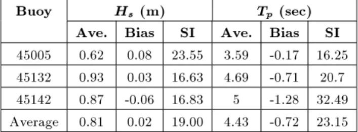
Table 3. The summary of statistical analysis of wave prediction by SWAN model.
Buoy Hs (m) Tp (sec)
Ave. Bias SI Ave. Bias SI 45005 0.62 0.08 23.55 3.59 -0.17 16.25 45132 0.93 0.03 16.63 4.69 -0.71 20.7 45142 0.87 -0.06 16.83 5 -1.28 32.49 Average 0.81 0.02 19.00 4.43 -0.72 23.15
the other hand, the SWAN model slightly overestimates signicant wave height. In general, the average error of the model for wave height is less than that of the wave period. The scatter index of the model is about 19 and 23 percent for the prediction of wave height and period, respectively.
As seen in Figure 4, in the B45005 station, in some instances, the recorded wave height and period are zero. Considering the nonzero values before and after these times (in this buoy) and the concurrent nonzero value in B45132 and B45142, it seems that these zero values are not reliable. Besides, the wave heights below 0.5 meters in marine activities have negligible importance, especially for extreme wave analysis, and are usually ignored [30-32]. In addition, the relative error is higher in the measurement of small waves than large waves. Therefore, wave heights below 0.5 meters were eliminated and error statistics were computed again. The corresponding results are shown in Table 4. According to Tables 3 and 4, the errors of the model for the prediction of wave height and period reduced about 3 percent after the elimination of small waves. This could be due to a non-clear mechanism for the generation of these waves and a possible error in their measurement.
As seen in Tables 3, 4 and Figure 5, the error for the prediction of wave height in station 45005 is more than those in stations 45132 and 45142. This could be due to several small islands, which are located near this station (Figure 1). These islands aect the wave regime next to them, which could not be properly modeled by the SWAN model. This is probably the reason for the larger error in station 45005.
Generally, these results are in agreement with
Table 4. The summary of statistical analysis of wave prediction by SWAN model for wave heights greater than 0.5 meter.
Buoy Hs(m) Tp (sec)
Ave. Bias SI Ave. Bias SI 45005 0.79 0.06 18.16 3.94 -0.22 12.36 45132 1.09 0.01 14.66 5.06 -0.79 18.65 45142 1.01 -0.08 15.35 5.28 -1.23 28.12 Average 0.96 0.00 16.06 4.76 -0.75 19.71
those of Lin et al. [10] that have used the SWAN model for wave simulation in the Chesapeake Bay. In their simulation, the SWAN has overestimated Hsand underestimated Tp and the accuracy of the model for the prediction of wave height is better than that of the wave period. However, the accuracy of our results is more than theirs. This could be due to several reasons. First, Lin et al. [10] have used the SWAN model for Chesapeake Bay, which is a shallow water body, and the depths in their stations were 3, 3.6 and 8.5 meters. In shallow waters, more parameters inuence the wave generation and transformation such as bottom friction and triad wave interaction. The second reason could be that most Hsvalues in their data set were less than 1 meter and, as we showed, the accuracy of the model for small waves is less than that for larger waves. Another reason could also be the frequency resolution of their simulation, which was 20 frequencies. This can also limit the accuracy of the SWAN model in prediction of Tp.
Another optional formulation for whitecapping in SWAN is the Cumulative Steepness Method (CSM), as described in Alkyon et al. [19]. In this method, dissipation due to whitecapping depends on the steep-ness of the wave spectrum at and below a particular frequency. Since the CSM method in SWAN is still in its experimental phase, we have evaluated it in this study. Tables 5 and 6 show the results for the whole studied period and after removing wave heights less than 0.5 meters, respectively.
According to Tables 3 to 6, using the cumulative steepness method for whitecapping dissipation yields
Table 5. The summary of statistical analysis of wave prediction by SWAN model with cumulative steepness method.
Buoy Hs(m) Tp (sec)
Ave. Bias SI Ave. Bias SI 45005 0.62 0.09 24.02 3.59 0.19 17.27 45132 0.93 -0.04 23.61 4.69 -0.27 15.23 45142 0.87 -0.11 24.66 5 -0.68 23.57 Average 0.81 -0.02 24.10 4.43 -0.25 18.69
Table 6. The summary of statistical analysis of wave prediction by SWAN model with cumulative steepness method for wave heights greater than 0.5 meter.
Buoy Hs(m) Tp (sec)
Ave. Bias SI Ave. Bias SI 45005 0.79 0.06 17.47 3.94 0.13 11.82 45132 1.09 -0.08 21.49 5.06 -0.37 12.39 45142 1.01 -0.15 22.77 5.28 -0.73 21.44 Average 0.96 -0.06 20.58 4.76 -0.32 15.22
worse results for signicant wave height and better results for the peak spectral period. By using this method, the average scatter index for prediction of Hs increases about 5 percent for both whole data and wave heights greater than 0.5 meters. Oppositely, the average scatter index for prediction of Tp decreases more than 4 percent by using the cumulative steepness method. It should be mentioned that the computa-tional time by using this option is longer than that when using the Komen [13] option. In our case, the required simulation time for 24 hours was about 13 minutes with the Komen [13] option and about 29 minutes when using the cumulative steepness method. Hence, the use of this method is not suggested for this case.
SUMMARY AND CONCLUSIONS
In this study, wind and wave characteristics on Lake Erie were investigated, based on the analysis of mea-surements at 3 buoys over 276 hours.
The obtained results are summarized as follows: The SWAN model showed fairly good capacity in
predicting the variations of Hs and Tp when wind suddenly changes direction and speed.
The SWAN model slightly overestimated signicant wave height and underestimated the peak spectral period. The average Bias parameter for Hswas 0.02 m and for Tp it was -0.72 s. The scatter indices were 19% and 23.15% for signicant wave height and the peak spectral period, respectively. Hence, the accuracy of the SWAN model was better in simulating wave height than wave period.
By eliminating data with wave heights less than 0.5 meters, the accuracy of the results improved. The error of the model for the prediction of wave height and period reduced about 3 percent.
Using the cumulative steepness method for white-capping dissipation yields worse results for sig-nicant wave height and better results for peak spectral period estimation. By using this method, the average scatter index for the prediction of Hs increased about 5 percent and for Tp decreased more than 4 percent. Also, the computational time required in this option was about more than twice the time in the Komen option.
ACKNOWLEDGMENT
We acknowledge the help of the National Data Buoy Center and Marine Environmental Data Service for their data. We would also like to express our grateful-ness to the SWAN group at Delft University of Tech-nology (Department of Fluid Mechanics) for proving
the model, and to two anonymous reviewers for their in sightful comments on this manuscript.
REFERENCES
1. Bretschneider, C.L. \Wave forecasting relations for wave generation", Look Lab., Hawaii, 1(3) (1970). 2. Wilson, B.W. \Numerical prediction of ocean waves
in the North Atlantic for December, 1959", Deutsche Hydrographische, Z.18(3), pp. 114-130 (1965). 3. Hasselmann, K., Barnett, T.P., Bouws, E., Carlson,
H., Cartwright, D.E., Enke, K., Weing, J.A., Gienapp, H., Hasselmann, D.E., Kruseman, P., Meerburg, A., Muller, P., Olbers, K.J., Richter, K., Sell, W. and Walden, W.H. \Measurements of wind-wave growth and swell decay during the joint north sea wave project (JONSWAP)", Deutsche Hydrograph, Zeit., Erganzung-Self Reihe, A8(12) (1973).
4. Donelan, M.A. \Similarity theory applied to the fore-casting of wave heights, periods and directions", In Proceedings of Canadian Coastal Conference, National Research Council of Canada, pp. 47-61 (1980). 5. Donelan, M.A., Hamilton, J. and Hui, W.H.
\Direc-tional spectra of wind-generated waves", Philos. Trans. R. Soc. Lond., A315, pp. 509-562 (1985).
6. U.S. Army, Shore Protection Manual, 4th Edn., 2vols. U.S. Army Engineer Waterways Experiment Station, U.S. Government Printing Oce, Washington, DC (1984).
7. U.S. Army \Coastal Engineering Manual", Chapter II-2, Meteorology and Wave Climate, Engineer Manual 1110-2-1100, U.S. Army Corps of Engineers, Washing-ton, DC (2003).
8. Booij, N., Ris, R.C. and Holthuijsen, L.H. \A third-generation wave model for coastal regions. 1. Model description and validation", Journal of Geophysical Research, 104, pp. 7649-7666 (1999).
9. Ris, R.C., Holthuijsen, L.H. and Booij, N. \A third-generation wave model for coastal regions. 2. Verica-tion", Journal of Geophysical Research, 104, pp. 7667-7681 (1999).
10. Lin, W., Sanford, L.P. and Suttles, S.E. \Wave mea-surement and modeling in Chesapeake Bay", Conti-nental Shelf Research, 22, pp. 2673-2686 (2002). 11. Ou, S.H., Liau, J.M., Hsu, T.W. and Tzang, S.Y.
\Simulating typhoon waves by SWAN wave model in coastal waters of Taiwan", Journal of Ocean Engineer-ing, 29, pp. 947-971 (2002).
12. Snyder, R.L., Dobson, F.W., Elliott, J.A. and Long, R.B. \Array measurement of atmospheric pressure uctuations above surface gravity waves", Journal Fluid Mech., 102, p.p 1-59 (1981).
13. Komen, G.J., Hasselmann, S., and Hasselmann, K. \On the existence of a fully developed wind sea spectrum", Journal Phys. Oceanography, 14, pp. 1271-1285 (1984).
14. WAMDI group \The WAM model - a third generation ocean wave prediction model", Journal Phys. Oceanog-raphy, 18, pp. 1775-1810 (1988).
15. Janssen, P.A.E.M. \Quasi-linear theory of wind-wave generation applied to wave forecasting", Journal Phys. Oceanography, 21, pp. 1631-1642 (1991).
16. Komen, G.J., Cavaleri, L., Donelan, M., Hasselmann, K., Hasselmann, S. and Janssen, P.A.E.M., Dynamics and Modelling of Ocean Waves, Cambridge University Press, p. 532 (1994).
17. Cavaleri, L. and Malanotte-Rizzoli, P. \Wind wave prediction in shallow water: Theory and applications", Journal of Geophysical Research, 86(C11), pp. 10961-10973 (1981).
18. Hasselmann, K. \On the spectral dissipation of ocean waves due to whitecapping", Bound.-Layer Meteor., 6(1-2), pp. 107-127 (1974).
19. Alkyon and Delft Hydraulics \SWAN fysica plus", Report H3937/A832 by order of RIKZ/RWS as a part of the project HR-Ontwikkeling (2002).
20. Collins, J.I. \Prediction of shallow water spectra", Journal of Geophysical Research, 77(15), pp. 2693-2707 (1972).
21. Madsen, O.S., Poon, Y.K. and Graber, H.C. \Spectral wave attenuation by bottom friction: Theory", Proc. 21th Int. Conf. Coastal Engineering, ASCE, pp. 492-504 (1988).
22. Hasselmann, S., Hasselmann, K., Allender, J.H. and Barnett, T.P. \Computations and parameterizations of the nonlinear energy transfer in a gravity wave spectrum. Part II: Parameterizations of the nonlinear transfer for application in wave models", Journal Phys. Oceanography, 15 (11), pp. 1378-1391 (1985).
23. Eldeberky, Y. and Battjes, J.A. \Parameterization of triad interactions in wave energy models", Proc. Coastal Dynamics Conf. '95, Gdansk, Poland, pp. 140-148 (1995).
24. Eldeberky, Y. \Nonlinear transformation of wave spec-tra in the nearshore zone", Ph.D. Thesis, Delft Univer-sity of Technology, Department of Civil Engineering, The Netherlands (1996).
25. Eldeberky, Y. and Battjes, J.A. \Spectral modeling of wave breaking: Application to Boussinesq equations", Journal of Geophysical Research, 101(C1), pp. 1253-1264 (1996).
26. Battjes, J.A. and Janssen, J.P.F.M. \Energy loss and set-up due to breaking of random waves", Proc. 16th Int. Conf. Coastal Engineering, ASCE, pp. 569-587 (1978).
27. Booij, N., Haagsma, IJ.G., Holthuijsen, L.H., Kieften-burg, A.T.M.M., Ris, R.C., Van der Westhuysen, A.J. and Zijlema, M. \SWAN User Manual", Cycle III version 40.41, Delft University of Technology, Delft (2004).
28. Kazeminezhad, M.H., Etemad-Shahidi, A. and Mousavi, S.J. \Evaluation of Neuro fuzzy and numer-ical wave prediction models in Lake Ontario", Journal of Coastal Res., SI50, pp. 317-321 (2007).
29. Westhuysen, A.J., Zijlema, M. and Battjes, J.A. \Nonlinear saturation-based whitecapping dissipation in SWAN for deep and shallow water", Journal of Coastal Eng., 54, pp. 151-170 (2007).
30. Kazeminezhad, M.H., Etemad-Shahidi, A. and Mousavi, S.J. \Application of fuzzy inference system in the prediction of wave parameters", Journal of Ocean Eng., 32, pp. 1709-1725 (2005).
31. Bishop, C.T. \Comparison of manual wave prediction models", Journal Waterway Port Coastal Ocean Eng., ASCE, 109(1), pp. 1-17 (1983).
32. Kamphuis, J.W. \Introduction to coastal engineering and management", Volume 16 of advanced series on ocean engineering, 1st Ed., World Scientic Pub. Co., pp. 81-100 (2000).