c
Sharif University of Technology, August 2009
Elitist-Mutated Ant System Versus
Max-Min Ant System: Application to
Pipe Network Optimization Problems
M.H. Afshar
1Abstract. The Ant Colony Optimization Algorithm (ACOA) is a new class of stochastic search algorithm proposed for the solution of combinatorial optimisation problems. Dierent versions of ACOA are developed and used with varying degrees of success. The Max-Min Ant System (MMAS) is recently proposed as a remedy for the premature convergence problem often encountered with ACOAs using elitist strategies. The basic concept behind MMAS is to provide a logical balance between exploitation and exploration. The method, however, introduces some additional parameters to the original algorithm, which should be tuned for the best performance of the method adding to the computational requirement of the algorithm. An alternative method to MMAS is proposed in this paper and applied to pipe network optimization problem. The method uses a simple but eective mechanism, namely Pheromone Trail Replacement (PTR), to make sure that the global best solution path has always the maximum trail intensity. This mechanism introduces enough exploitation into the method and more importantly enables one to exactly predict the number of global best solutions at each iteration of the algorithm without requiring calculation of the cost of the solutions created. The sub-colony of repeated global best solutions of the iterations is then mutated, such that a predened number of solutions survive the mutation process. Two dierent mutation mechanisms, namely deterministic and stochastic mutation processes, are introduced and used. The rst one uses a one bit mutation with a probability of one on some members of the sub-colony, while the second one uses a uniform mutation on the whole sub-colony. The probability of mutation in the second mutation process is adjusted at each iteration, so that the required number of global-best solutions survives the mutation. The method is shown to produce results comparable to the MMAS algorithm, while requiring less free parameter tuning. The application of the method to a benchmark example in the pipe network optimization discipline is presented and the results are compared.
Keywords: Mutated; Ant colony optimization algorithm; Pipe networks; Optimal design.
INTRODUCTION
Ant Colony Optimization (ACO) is a general frame-work for developing optimization algorithms based on the collective behaviour of ants in their search for food [1]. These algorithms were initially inspired by the observation that ants can nd the shortest paths between food sources and their nest even though they are almost blind. Individual ants choose their paths from the nest to the food source in an essentially random fashion [2]. While walking from food sources
*. Department of Civil Engineering, Iran University of Science and Technology, Tehran, P.O. Box 16765-163, Iran. E-mail: [email protected]
Received 15 December 2007; received in revised form 28 April 2008; accepted 8 September 2008
to the nest and vice versa, however, ants deposit on the ground a substance called pheromone forming in this way a pheromone trail. Ants can smell pheromone and, when choosing their way, they tend to choose in probability paths marked by strong pheromone concentrations. The pheromone trail acts as a form of indirect communication called stigmergy [3] helping the ants to nd their way back to the food source or to the nest. Also, it can be used by other ants to nd the location of the food sources found by their nest mates. It has been shown experimentally [4] that this pheromone trail following behavior can give rise, once employed by a colony of ants, to the emergence of shortest paths.
The searching behavior of Ant Colony Optimiza-tion Algorithms (ACOA) can be characterized by two main features [5]; exploration and exploitation.
Explo-ration is the ability of the algorithm to broadly search through the solution space, while exploitation is the ability of the algorithm to search thoroughly in the lo-cal neighborhood where good solutions have previously been found. Higher exploitation is reected in the rapid convergence of the algorithm to a suboptimal solution while higher exploration results in a better solution at higher computational cost due to the slow convergence of the method. By denition, these attributes are in conict with one another. A trade-o between explo-ration and exploitation in ant algorithms is, therefore, vital for a logical balance between the optimality of the solution and the eciency of the method. To encourage exploitation, techniques have been adopted to ensure that information about the best solutions govern the search process. Bullnheimer et al. [6] suggested an elitism strategy, where information about the best solution is emphasized in the algorithms' search pro-cedure. Dorigo and Gambardella [7] used a technique to conne the search to the local neighborhood of the best solution. Dorigo et al. [8] used local optimizers to further improve good solutions. The biggest problem that can be caused by such exploitative methods is insucient exploration and premature convergence to sub-optimal solutions. Dierent remedies, in the form of anti-convergence techniques, are suggested for premature convergence phenomena often encountered when using these exploitative methods. The most notable of these methods is the Max-Min Ant System (MMAS) proposed by Stutzle and Hoos [9] in which the pheromone trails are adjusted at each iteration such that no one solution dominates the stochastic selection process. Afshar [10] has recently proposed an alternative form of the ant's stochastic decision policy, which overcomes the stagnation phenomena often encountered with the algorithms using an elitist strategy. The proposed method has the advantage of not introducing a free parameter while producing comparable results with other anti-stagnation methods. A new anti-stagnation method is proposed in this paper to be used with the elitist strategy of pheromone updating in ACO algorithms. The method is based on the observation that at the stagnation point, the colony is dominated by one solution, which may or may not be the global best solution of the search depending on the pheromone updating procedure used. The proposed method uses a Pheromone Replacement Mechanism (PRM) to ensure that the colony is only dominated by the global best solution when stagnation occurs. This mechanism is advantageous, as it enables one to exactly calculate the number of global best solutions created at each iteration. The global best solutions of the iteration are mutated such that a predened number of these solutions survive the mutation process. Two dierent mutation mechanisms, namely deterministic and probabilistic mutations, are devised and used. The
proposed method is used here in conjunction with the ant system using the elitist strategy and, hence the name Elitist Mutated Ant System (EMAS) is used for the resulting algorithm. Application of the proposed method to one of the benchmark problems in the pipe network optimization literature is addressed and the results are compared with that of MMAS. The experiments show the proposed method is able to produce comparable results to that of MMAS while introducing less free parameters.
ANT COLONY OPTIMIZATION ALGORITHM
In the Ant Colony Optimization (ACO) meta-heuristic, a colony of articial ants cooperates in nding good solutions to discrete optimization problems. Applica-tion of the ACO algorithm to arbitrary combinatorial optimization problems requires that the problem be projected on a graph [7]. Consider a graph, G = (D; L; C), in which D = fd1; d2; ; dng is the set
of decision points at which some decisions are to be made, L = flijg is the set of options, j = 1; 2; ; J, at
each of the decision points, i = 1; 2; ; n, and nally C = fcijg is the set of costs associated with options
L = flijg. The components of sets D and L may be
constrained if required. A path on the graph is called a solution (') and the minimum cost path on the graph is called the optimal solution ('). The cost of a solution
is denoted by f(') and the cost of the optimal solution by f(').
The basic steps in ACO algorithms [2] may be dened as follows:
1. m ants are randomly placed on the n decision points of the problem and the amount of pheromone trail on all options are initialized to some proper value at the start of the computation;
2. A transition rule is used for ant k at each decision point i to decide which option is to be selected. Once the option at the current decision point is selected, the ant moves to the next decision point and a solution is incrementally created by ant k as it moves from one point to the next. This procedure is repeated until all decision points of the problem are covered and a complete solution is constructed by ant k. The transition rule used in the original ant system is dened as follows [2]:
pij(k; t) = [ij(t)] [
ij] J
P
j=1[ij(t)] [ij]
; (1)
where pij(k; t) is the probability that ant k selects
option lij(t) for the ith decision at iteration t; ij(t)
at iteration t; ij = (c1ij) is the heuristic value
representing the cost of choosing option j at point i, and and are two parameters that control the relative weight of the pheromone trail and heuristic value referred to as the pheromone and the heuristic sensitivity parameter, respectively. The heuristic value, ij, is analogous to providing the ants with
sight and is sometimes called visibility. This value is calculated once at the start of the algorithm and is not changed during the computation. The role of parameters and can be best described as follows: If = 0, the cheapest options are more likely to be selected, leading to a classical stochastic greedy algorithm. If, on the contrary, = 0, only pheromone amplication is at work, which will lead to the pre-mature convergence of the method to a strongly sub-optimal solution [2];
3. The cost, f('), of the trial solution generated is calculated. The generation of a complete trial solution and calculation of the corresponding cost is called a cycle (k);
4. Steps 2 and 3 are repeated for all m ants of the colony at the end of which m trial solutions are created and their costs are calculated. Generation of m trial solutions and calculation of their corre-sponding costs is referred to as an iteration (t); 5. The pheromone is updated at the end of each
iteration. The general form of the pheromone updating used in the ant system is as follows [2]:
ij(t + 1) = ij(t + 1) + ij; (2)
where ij(t + 1) is the amount of pheromone trail
on option j of the ith decision point, i.e. option lij at iteration t + 1; ij(t) is the concentration of
pheromone on option lij at iteration t; 0 1 is
the coecient representing pheromone evaporation, and ij is the change in pheromone
concentra-tion associated with opconcentra-tion lij. The amount of
pheromone trail, ij(t), associated with option lij
is intended to represent the learned desirability of choosing option j when in decision point i. The pheromone trail information is changed during the problem solution to reect the experience acquired by the ants during problem solving. The main role of pheromone evaporation is to avoid stagnation, that is, the situation in which all ants end up doing the same tour. In addition, evaporation reduces the likelihood that high cost solutions will be selected in future cycles.
Dierent methods are suggested for calculating pheromone change. In the original ant system sug-gested by Dorigo et al. [2], all ants deposit pheromone on the options they have selected to produce the
solution, ij=
m
X
k=1
k
ij; (3)
in which k
ij is the pheromone deposited by ant k on
option lijduring iteration t. The amount of pheromone
change is usually dened as [2]:
k
ij=
(
R
f(')k if option (i; j) is chosen by ant k
0 otherwise (4)
where f(')k is the cost of the solution produced by ant
k, and R is a quantity related to the pheromone trail, called the pheromone reward factor. The amount of pheromone added to each of the options during a cycle is a function of the cost of the trial solution generated. The better the trial solution, and hence the lower the cost, the larger the amount of pheromone added to the option. Consequently, solution components that are used by the best ant and which form a part of the lower cost solution receive more pheromone and are more likely to be selected by future ants. This choice clearly helps to direct the search towards good solutions.
At the end of each iteration, each ant has gener-ated a trial solution. The pheromone is updgener-ated before the next iteration starts. This process is continued until the iteration counter reaches its maximum value dened by the user. A note has to be added regarding the feasibility of the solutions created by ants in con-strained optimization problems. If the constraints can be explicitly dened in terms of the options available at a decision point, the ants are forced to create feasible solutions by limiting the available options to those leading to feasible solutions. In TSP, for which the ant algorithms were originally devised and were tested on, the feasibility of the solution requires that each point is visited once and only once and that the nishing point is the same as the starting one. This is not, however, possible in optimization problems such as pipe network optimization problems, where the constrained are implicitly dened in terms of the options and, therefore, the feasibility of the solution is only known when the solution is totally created. In these problems, a higher total cost is usually associated to the infeasible solutions via use of a penalty function to discourage the ants from taking options which constitute parts of these solutions.
ELITIST STRATEGIES
In the ant system described in the previous section, all the ants contribute to the pheromone change cal-culation dened by Equation 3. This means that options that have been selected before will have a
higher chance of selection in future iterations. This pheromone updating rule is of a highly explorative nature. The exploitation, on the other hand, is only reected in Equation 4, where the pheromone changes caused by better solutions are calculated to be higher than other solutions. The experience shows, however, that the exploitation introduced into the method by Equation 4 is not enough to balance the exploration present in the algorithm. This is usually reected in slower convergence of the method or convergence to the sub-optimal solutions depending on the value of the evaporation factor used. Dierent methods are suggested to regulate a trade-o between the exploitation of the best solutions (iteration-best and global-best) and further exploration of the solution space. Dorigo and Gambardella [7] presented the Ant Colony System (ACS), which includes additional rules that probabilistically determine whether an ant is to act in an exploitative or explorative manner at each decision point. Another mechanism used within ACS is the local updating of the pheromone of the ant's selected options immediately after it has generated its solution, such that the reselection of options within an iteration is discouraged, leading to further exploration of the method. The global updating rule in ACS is similar to that in AS, but in ACS, only the path with the global-best solution receives additional pheromone. This updating rule clearly acts as an encouragement for exploitation, as only the best solution is reinforced with additional pheromone. To exploit information about the global-best solution, Dorigo et al. [2] proposed the use of an algorithm known as the Elitist Ant System (ASelite). The updating rule in ASelite is the same as
that of AS, except that in ASelite the global-best ant is
also allowed to contribute to the pheromone change times at each iteration. The updating rule for ASelite
encourages both exploration (as each of the m solutions found by the colony receive a pheromone addition) and exploitation, as the global-best path is reinforced with the greatest amount of pheromone. As ! 1, the emphasis on exploitation is greater. Another method further developing the idea of elitism is the elitist-Rank Any System (ASrank) proposed by Bullnheimer
et al. [6], which involves a rank-based updating scheme. At the end of an iteration, elitist ants reinforce the current global best path, as in ASelite, and the ants that
found the top 1 solutions within the iteration add pheromone to their paths with a scaling factor related to the rank of their solution. The decision rule for the ASrank is the same as that for AS.
MAX-MIN ANT SYSTEM
Max-Min Ant System (MMAS) suggested by Stutzle and Hoos [9] is yet another method that employs the idea of elitism to introduce exploitation into the
original ant system. The provision of exploitation is made in MMAS by the addition of pheromone to only the iteration-best ant's path at the end of each iteration. To further exploit good information, MMAS uses the global-best solution to update the pheromone trail every Tgbiterations. The MMAS updating scheme
is then given by:
ij(t) = ijib(t) + ijgb(t)INft=Tgbg; (5)
where N is the set of natural numbers and ib ij(t)
and ijgb(t) are the pheromone addition given by the iteration-best and global-best ants, respectively.
Premature convergence to sub-optimal solutions is an issue that can be experienced by all ACO algo-rithms, especially those that use an elitist strategy of pheromone updating. To overcome this problem, whilst still allowing for exploitation, Stutzle and Hoos [9] proposed the provision of dynamically evolving bounds on pheromone trail intensities such that the pheromone intensity on all paths is always within a specied range. As a result, all paths will have a non-trivial probability of being selected and, thus, a wider exploration of the search space is encouraged. MMAS uses upper and lower bounds to ensure that pheromone intensities lie within a given range, which is calculated based on some analytical reasoning. The upper pheromone bound at iteration t is given by [9]:
max(t) = 1 1 f(')Rgb: (6)
This expression is equivalent to the asymptotic pheromone limit of an option receiving a pheromone addition of R=f(')gband decaying by a factor of 1 at
the end of each iteration. The upper bound as dened in Equation 6, was found to be of lesser importance, while the lower limit played a more decisive role. Stutzle and Hoos [9] introduced the following formula for the calculation of the lower trail strength limit based on some analytical arguments:
min= max:(1 p dec)
(Javg 1):pdec; p
dec= (pbest)1=n; (7)
where minrepresents the lower limit for the pheromone
trail strength; pdec is the probability that an ant
constructs each component of the best solution again; pbest is the probability that the best solution is
con-structed again and Javg is the average number of
options available at decision points of the problem. MMAS, as formulated in Stutzle and Hoos [9], also incorporates another mechanism known as Pheromone Trail Smoothing (PTS). This mechanism reduces the relative dierence between pheromone intensities and further encourages exploration. The PTS operation performed at the end of each iteration is given by:
where 0 1 is the PTS coecient. If = 0, the PTS mechanism has no eect whereas if = 1, all pheromone trails are scaled up to max(t). In addition
to these additional mechanisms, MMAS uses the same decision policy as AS.
PIPE NETWORK OPTIMIZATION
Due to the high costs associated with pipe networks, much research over the last decades has been dedicated to the development of methods to minimize the capital costs associated with such an infrastructure. Within the last decade, many researchers have shifted the focus of pipe network optimization from traditional techniques based on linear and nonlinear programming to the implementation of heuristic methods derived from nature [5] namely: Genetic Algorithms (GAs) [11-16], simulated annealing [17] and Ant Colony Opti-mization (ACO) [10,18,19]. The pipe network opti-mization problem in its simplest form is dened as selecting the diameter of each pipe of the network so that the resulting network has a minimum cost while meeting the required conditions. These conditions are often considered as pipe velocities and nodal pressures remaining in a pre-specied range dened by maximum and minimum velocity and pressure values. Here, each pipe is a decision point at which the diameter of the pipe is to be determined. The components of the decision set, D = fd1; d2; di; ; dng, are, therefore,
the existing pipes of the network, where di represents
the ith pipe of the network. The pipe diameters are usually selected from a set of commercially available diameters, ' = f'ijg, which may or may not be
the same for all the pipes. Assuming that these diameters are the same for all the pipes, then ' = ('1; '2; ; 'J) would represent the list of available
options at each and every decision point of the problem. If ucj is dened as the per unit length cost of the pipe
with diameter 'j, cost cij associated to option 'j at
decision point di can now be calculated as the product
of per unit cost ucj and length lei of the link under
consideration. The cost of a trial solution, f('), which may or may not be a feasible solution, is now calculated as the sum of the links cost plus a penalty term dened as:
f(') =Xn
i=1
ucj lei+ pCSV; (9)
CSV = ( n
X
i=1
1 VVi
min
+Xn
i=1
Vi
Vmax 1
+Xnn
in=1
1 HHin
min
+Xnn
in=1
Hin
Hmax 1
) ;
in which n and nn are the number of existing pipes and nodes, respectively; Hin is the nodal head; Hmin
and Hmax are minimum and maximum allowable
hy-draulic head; Vi is the pipe velocity; Vmin and Vmax
are minimum and maximum allowable ow velocity; CSV represents a measure of the head and velocity constraint violation of the trial solution and p is the
penalty parameter with a large enough value to ensure that any infeasible solution will have a higher total cost than any feasible solution. It should be noted that in calculating the CSV , the summation ranges over those nodes and pipes at which a violation of pressure and velocity constraints occurs, i.e. the terms in each parenthesis are positive. Here, the penalty parameter is taken as the cost of the most expensive network, i.e. a network with all its pipes having the largest possible diameter. For a given network, the nodal pressures and pipe velocities are obtained via the use of a simulation program that explicitly solves the set of hydraulic constraints for nodal heads [20]. This, however, requires the denition of some parameters in the Hazen-Williams equation, which states the relation between head loss and ow in each link. Here, a Hazen-Williams formula of the type:
hf = L
Q C
D ; (10)
is used, in which L = length of pipe; Q = ow rate of pipe; C = Hazen-Williams coecient, D = internal diameter of pipe and: = 1:852, = 4:871 and = 10:667 for q in cubic meters per hour and d in inches (equivalent to = 4:727 for D in feet and Q in cubic feet per second) are Hazen-Williams constants as used in EPANET 2.0.
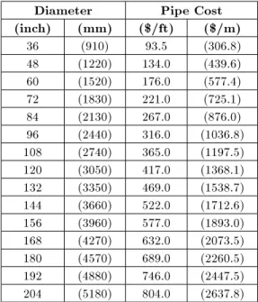
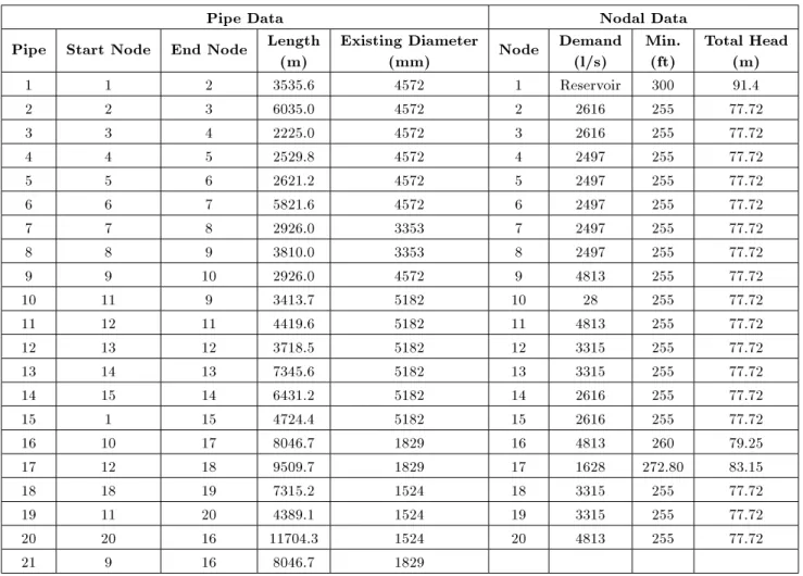
The test problem considered here concerns the rehabilitation of the New York City water supply network with 21 pipes, 20 demand nodes and one reservoir as shown in Figure 1 [11]. The commercially available pipe diameters and their respective costs are listed in Table 1, while the pipe and nodal data of the existing network are shown in Table 2. This table is augmented by a virtual zero-diameter cost equal to half of the cheapest diameter to enable the calculation of local heuristics for all available options. This problem has been used as a case study by many researchers using genetic algorithms [11,12,15,16,21]; most recently by Maier et al. [18]; Zecchin et al. [22] and Afshar [10] using ACO algorithms.
ELITIST-MUTATED ANT SYSTEM (EMAS) MMAS, as dened above, suers from some shortcom-ings. Firstly, the argument behind MMAS is based on the strong assumption that around good solutions other good or even better solutions are located. This
Figure 1. New York tunnel network.
Table 1. Pipe cost data for New York network. Diameter Pipe Cost (inch) (mm) ($/ft) ($/m)
36 (910) 93.5 (306.8) 48 (1220) 134.0 (439.6) 60 (1520) 176.0 (577.4) 72 (1830) 221.0 (725.1) 84 (2130) 267.0 (876.0) 96 (2440) 316.0 (1036.8) 108 (2740) 365.0 (1197.5) 120 (3050) 417.0 (1368.1) 132 (3350) 469.0 (1538.7) 144 (3660) 522.0 (1712.6) 156 (3960) 577.0 (1893.0) 168 (4270) 632.0 (2073.5) 180 (4570) 689.0 (2260.5) 192 (4880) 746.0 (2447.5) 204 (5180) 804.0 (2637.8)
is denitely the case for TSP, the problem for which the MMAS is proposed, as it is shown that reason-ably good tours are located in a small region of the search space. This is not necessarily true for other problems such as pipe network optimization problems in which good solutions may be surrounded by costly
infeasible solutions. The second is that the trail limits and, in particular, the lower limit used in MMAS will eectively come into play when a best found solution dominates the colony to encourage the ant to create some other solutions using the components of this solution. When an elitist strategy is used for pheromone updating, the trail intensities on all the options available at an arbitrary decision point are nearly zero except for the option corresponding to the best found solution. MMAS calculates the lower bound of the trail intensities for a given value of pbest and
raises the near-zero value of all options to this value. At this moment, all the options except one will have the same non-zero trail intensity. This will of course increase the chance of other options to constitute part of the next iteration solutions but in a random fashion. The ants will be required to take a random walk in an articially widened search space around the dominating solution. And, nally, the MMAS introduces some additional free parameters such as pbest, Tgb and
in addition to , , , Q and m, which are used by all ACO algorithms. While some heuristics are derived for the rst set of parameters [19], the setting of the second set is subject to trial and error. The value of these parameters should be tuned for the best performance of the algorithm prior to the main application of the method. This, of course, adds to the computational requirements of MMAS compared to those of the original ant system.
To introduce the proposed method, rst consider the role of the additional parameters, pbest, T
gb and
used in MMAS. Parameters pbestand are both meant
to introduce exploration into the algorithm as dened earlier. The exploration increases with the decreasing value of pbest and the increasing value of . These
parameters are not, however, independent. Assuming that the PTS operation dened by Equation 8 is followed by the implementation of Equation 7 using predened pbest, then it is highly probable that for
large enough values of PTS parameter, , the smoothed pheromone trails calculated by Equation 8 will be higher than the lower bound mindened by Equation 7
leading to the redundancy of this equation. If, on the other hand, the PTS operation is preceded by the implementation of pbest, then the PTS mechanism leads
to a mere constant scaling of the calculated minimum pheromone trails, min, on the options which do not
constitute a part of the dominating solution. This eect can be clearly achieved by using a lower value of pbestwithout having to use the PTS mechanism. It
can, therefore, be argued that only one of these two mechanisms is needed to introduce the required explo-ration into MMAS. Parameter pbesthas the advantage
of easier setting as it carries a physical meaning, i.e. the probability that the best solution is created by all ants. It is, therefore, reasonable to disregard the
Table 2. Pipe and nodal data for New York tunnel network.
Pipe Data Nodal Data
Pipe Start Node End Node Length (m)
Existing Diameter
(mm) Node
Demand (l/s)
Min. (ft)
Total Head (m) 1 1 2 3535.6 4572 1 Reservoir 300 91.4 2 2 3 6035.0 4572 2 2616 255 77.72 3 3 4 2225.0 4572 3 2616 255 77.72 4 4 5 2529.8 4572 4 2497 255 77.72 5 5 6 2621.2 4572 5 2497 255 77.72 6 6 7 5821.6 4572 6 2497 255 77.72 7 7 8 2926.0 3353 7 2497 255 77.72 8 8 9 3810.0 3353 8 2497 255 77.72 9 9 10 2926.0 4572 9 4813 255 77.72 10 11 9 3413.7 5182 10 28 255 77.72 11 12 11 4419.6 5182 11 4813 255 77.72 12 13 12 3718.5 5182 12 3315 255 77.72 13 14 13 7345.6 5182 13 3315 255 77.72 14 15 14 6431.2 5182 14 2616 255 77.72 15 1 15 4724.4 5182 15 2616 255 77.72 16 10 17 8046.7 1829 16 4813 260 79.25 17 12 18 9509.7 1829 17 1628 272.80 83.15 18 18 19 7315.2 1524 18 3315 255 77.72 19 11 20 4389.1 1524 19 3315 255 77.72 20 20 16 11704.3 1524 20 4813 255 77.72 21 9 16 8046.7 1829
PTS operation by assuming a value of zero for and only tune pbestfor balancing the exploitation and
exploration of the MMAS.
Now, consider the eect of Tgb as used in
Equa-tion 5. This equation states that the global-best path should be reinforced every Tgb iteration. For
very large values of this parameter, only iteration-best solutions are used to update the pheromone trail. In this situation, it is possible that the search does not converge on a single solution or otherwise converge to a solution dierent from the global-best solution, depending on the value of the evaporation factor, , used. For the values of close to 1.0, MMAS may fail to converge and for small enough values of , stagnation at the sub-optimal solution may occur. In the rst case, implementation of Equation 7 will be redundant, since this mechanism comes into eect when stagnation starts to take place. Implementation of Equation 7 in the second case will lead to a search around a sub-optimal solution, which will clearly be inecient. Small values of Tgb, with a minimum value of one,
result in higher exploitation of the global-best solution, which is often reected in the colony being dominated by the current global-best solution. In other words,
the role of the Tgb is merely to ensure that the path
with maximum pheromone intensity corresponds to the current global-best solution at all stages of the search. An experiment is carried out at this stage to verify this interpretation of Tgb. The example problem is
solved with dierent values of Tgb = 1; 10 and 1 for
xed values of other parameters, = 1, = 0:25, = 0:98, m = 50 and pbest = 1:0. These values
are chosen following heuristics suggested by Zecchin et al. [19] and some preliminary runs. Figures 2 to 5 show the variations of the averaged number of Global-Best Solutions (GBS) and Maximum Pheromone Intensity Solutions (MPIS) during the search process for dierent values of Tgb obtained from ten runs using dierent
initial colonies. It is clearly seen from Figure 2 that for a large value of Tgb = 1, the number of GBS and
MPIS are dierent during the search process. The dierence increases as the solution corresponding to maximum pheromone intensity dominates the colony. This dierence indicates that a pheromone updating rule that only uses iteration-best solutions may lead to domination of a solution dierent from the global-best solution. It is obvious that implementation of Equation 7 with pbest < 1 will be inecient in this
Figure 2. Variation of the average number of GBS and MPIS with the number of evaluations for ten runs (Tgb= 1).
Figure 3. Variation of the average number of GBS and MPIS with the number of evaluations for ten runs (Tgb= 10).
situation. The dierence between the number of GBS and MPIS decreases with a decreasing value of Tgb as
illustrated in Figures 3 and 4. It can, therefore, be argued that the main eect of reinforcing the global-best path in MMAS is to make sure that the solution corresponding to maximum pheromone intensity is the current global-best solution of the search. In this situation, implementation of Equation 7 with pbest< 1
will result in a colony of solutions constructed on and around the global-best solution of the search. This, of course, increases the chance of improving the current GBS compared to a situation in which the colony is constructed on and around an inferior solution; a situation which happens for larger values of Tgb. It is also instructive to note that small values
of Tgb (reinforcing the global-best path more often)
will result in more exploitation, which is reected in faster stagnation of the search; an eect similar to that expected from the evaporation factor. This means that both evaporation factor and Tgb play an exploitative
role in MMAS. A successful implementation of the
Figure 4. Variation of the average number of GBS and MPIS with the number of evaluations for ten runs (Tgb= 1).
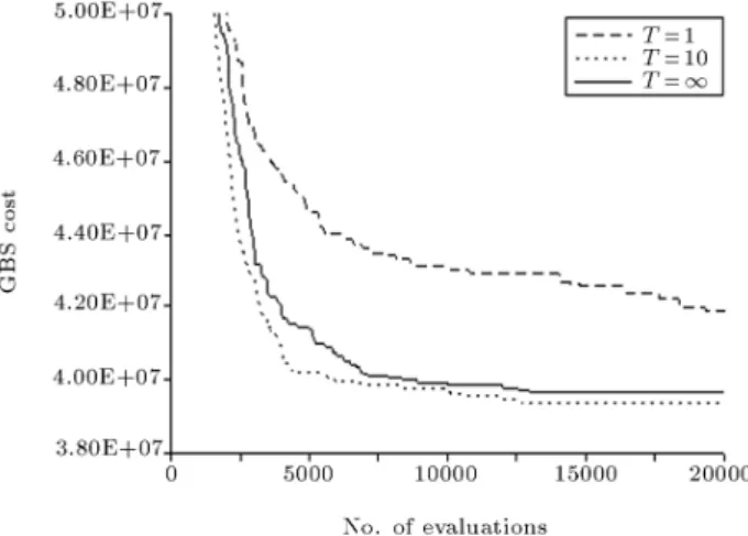
Figure 5. Variation of the average GBS cost for dierent values of Tgb.
algorithm, therefore, requires a careful tuning of these parameters to ensure that a) the colony has enough time to explore the search space before domination of MPIS, and b) the MPIS is the same as GBS so that the colony is dominated by the current GBS and not any other inferior solution. It is instructive to see the performances of MMAS for dierent values of parameter Tgb. Figure 5 shows the variation of average
GBS costs of ten runs using dierent initial colonies for Tgb= 1; 10, 1 and pbest= 0:05. The best performance
of the MMAS is achieved for Tgb = 10 in terms
of convergence characteristics and the quality of the solution. The algorithm shows the worst performance for Tgb = 1 due to higher exploitation which is not
balanced by the exploration introduced via the use of pbest = 0:05. MMAS using Tgb = 1 shows not only
inferior, though close, convergence behavior to MMAS using Tgb = 10, but also a lower success rate of 1 in
ten runs in locating the global solution of the problem, with a cost of $38.63M compared to the success rate of 3 achieved by the latter. This can be attributed to the fact that in the latter case, the maximum pheromone
intensity path does not correspond to the GBS in all ten runs as shown earlier in Figure 2. To complete the observations, another experiment is carried out to examine the convergence behavior of the algorithm for = 1, pbest = 1 and Tgb = 1; 10 and 1. The results,
not shown here, indicated that irrespective of the level of exploitation, the value of Tgb, the algorithm is not
convergent when no evaporation is present ( = 1). For all values of Tgb used, the average number of GBS
and MPIS was always below 2% of the colony size at all stages of the search. It is obvious that the introduction of further exploration via implementation of Equation 7 with pbest < 1 will be redundant in this situation. It
can, therefore, be argued that in MMAS, evaporation ( < 1) guarantees convergence; reinforcement of GBS with a proper value of Tgb ensures that the algorithm
converges on the GBS; and nally the adjustment of the lower pheromone bound with pbest < 1 enlarges
the search space around the GBS, providing the ants with the means to improve current GBS.
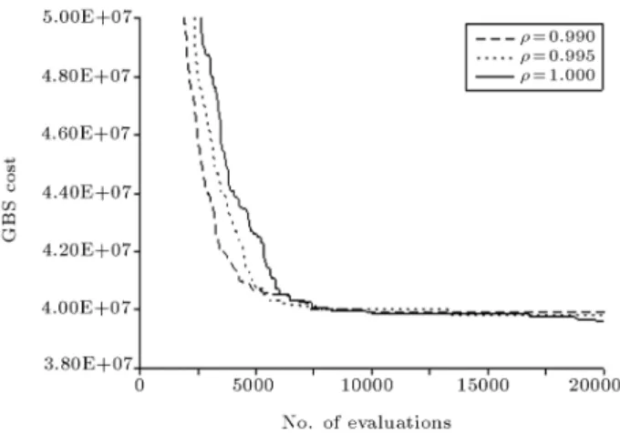
The proposed Elitist-Mutated Ant System (EMAS) uses the same decision policy as that of AS and a pheromone updating rule in which only iteration-best solutions are reinforced at each iteration. To ensure that the algorithm only converges to the GBS, EMAS uses a simple but eective parameter-free Pheromone Replacement Mechanism (PRM) in which the pheromone intensity of the GBS is replaced with that of the path dened by maximum pheromone intensity and vice versa whenever a new GBS is located. This will guarantee that the current global-best solution has the maximum pheromone trail and, therefore, has a very high chance of being selected as the iteration-best solution of the iteration to be used in the pheromone updating process. An experiment is carried out at this stage to verify the eectiveness of the proposed PRM. Figure 6 shows the average number of GBS and MPIS of ten runs
Figure 6. Variation of the average number of GBS during the search for dierent values of evaporation factor using PRM.
versus the number of iterations for three values of evaporation factor = 1, 0.995 and 0.99, with other parameters chosen as = 1, = 0:25, m = 50 and pbest = 1:0. It should be noted that each curve in
Figure 6 is representative of both the number of GBS and MPIS as these have been found to be virtually the same. It is interestingly seen that the PRM introduces enough exploitation into the algorithm, even when no evaporation, = 1, is introduced into the algorithm. The algorithm shows faster stagnation with decreasing values of evaporation factor as expected. The algorithm, however, has enough chance to explore the search space before stagnation starts, when no evaporation is used. The proposed PRM seems to be very advantageous, as it simulates the eect of both GBS reinforcement and evaporation without introducing any free parameter. It can therefore be expected that PRM with no or little evaporation performs better as the resulting search process will have enough time to explore the search space before stagnating at the current global-best solution. This expectation is indeed fullled as shown in Figure 7 where the average GBS cost is seen to decrease with an increasing value of the evaporation factor. The minimum average solution cost, in fact, is obtained when no evaporation is used. The proposed PRM, therefore, ensures enough exploitation and convergence of the method to the GBS solution irrespective of the amount of evaporation used. The averaged GBS costs and the success rate of the algorithm for the values of evaporation factor = 1, 0.995 and 0.99 were $39.61M,2, $39.82M,1 and $39.93M,1, respectively.
An explorative feature can now be introduced to balance the exploitation embedded in the algorithm, via use of PRM, to replace the lower bound scaling (Equation 7) of MMAS. This is achieved using the mutation mechanism commonly used in GAs on the sub-colony of current global-best solutions created at each iteration once the stagnation is started. Two
Figure 7. Variation of the average GBS cost for dierent values of evaporation factor using PRM.
mutation procedures, one deterministic and the other stochastic are introduced and used here. In the deterministic method, a one-bit mutation is carried out on (Mgb m:Pgb) of the global-best solutions at each
iteration where Pgb is the ratio of the number of
global-best solutions surviving the mutation set by the user and Mgb is the number of global-best solutions created
at each iteration. With the PRM used, the number of global-best solutions can be easily calculated by checking the colony against the maximum pheromone intensity path. In the second, stochastic method, all the Mgb global-best solutions undergo a uniform
mutation with probability Pm dened as:
Pm= 1
mMPgb
gb
1 n
; (11)
where n denotes the number of decision points of the problem and m is the colony size as dened earlier. The probability of mutation ensures that, on average, m:Pgb
of global-best solutions survive the mutation. It can be seen that the mutation mechanism is activated only when Mgb > m:Pgb in both of the methods. It should
be noted that Pgb carries a meaning similar to that of
Pbestused in MMAS. An experiment is now carried out
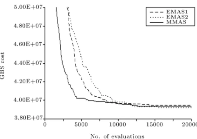
to verify the eciency of the proposed mutation mech-anisms. Figure 8 compares the variation of the average GBS cost, using rst and second mutation mechanisms denoted by EMAS1 and EMAS2, respectively, with that of the best performing MMAS. EMAS results were obtained using ve parameter values: = 1, = 0:25, = 1:0, Pgb = 0:05 and m = 50, while
MMAS required the tuning of six parameters as = 1, = 0:25, = 0:98, Tgb = 10, pbest = 0:05 and
m = 50. Considering the exploitative behavior of EMAS with no evaporation, there is actually no need to tune for the evaporation factor. The number of free parameters of EMAS, therefore, reduces to four, compared to six for MMAS. It is seen that the average
Figure 8. Variation of the average GBS cost for the best performing MMAS and proposed EMAS.
GBS cost obtained by EMAS1 ($39.44M) is marginally inferior to that of MMAS ($39.32M) while EMAS2 with an average GBS cost of $39.20M performs marginally better than MMAS. All three methods had a success rate of 3 out of ten in locating the optimum solution of $38.64M, which has been reported by other researchers using dierent methods [18,23]. It is obvious that the mutations introduced are responsible for improving the average GBS cost and the success rate of the PRM from $39.61M,2 to $39.44M,3 and $39.20M,3 obtained by EMAS1 and EMAS2, respectively. It is also instructive to compare the number of average global-best solutions for three algorithms as shown in Figure 9. It is clearly seen that both of the mutation mechanisms used in EMAS were successful to control the number of GBS around m:Pgb = 2:5 while this number is very high
for MMAS. This is, in fact, another feature of the proposed EMAS enabling the method to compete with MMAS using less tuning parameters. The proposed EMAS is, therefore, computationally less demanding than MMAS while producing comparable results. CONCLUDING REMARKS
A new ACO algorithm was presented as an alternative to the Max-Min Ant System. The method exploits automatically balanced exploitative and explorative features. The exploitation of the method is provided by a simple but eective free-parameter procedure in which the global-best solution pheromone intensity is replaced by the current maximum pheromone trail, each time the global-best solution is updated. This pro-cedure was shown to introduce enough exploitation into the method ensuring the convergence of the search to the global-best solution, irrespective of the value of the evaporation factor. The method oers the advantage of exactly predicting the number of global-best solutions of the iteration without requiring calculation of the cost of the trial solutions. Two mutation mechanisms, one
Figure 9. Variation of average number of GBS for best performing MMAS and proposed EMAS.
deterministic and the other stochastic, were then used on the predicted global-best solutions to introduce a balancing exploration into the algorithm. The deter-ministic approach uses a one-bit mutation on a number of global-best solutions while in the stochastic one, all the global-best solutions undergo a uniform mutation process with an automatically calculated probability. Both of the mutation procedures were devised such that a predened number of global-best solutions survive the mutation. The proposed algorithm was tested against a benchmark example in the water distribution network optimization literature and the results compared with that of MMAS. The results show that the proposed algorithm produces solutions comparable to that of MMAS, while introducing less free parameters to be tuned.
REFERENCES
1. Dorigo, M. and Di Caro, G. \The ant colony optimiza-tion meta-heuristic", New Ideas in Optimizaoptimiza-tion, D. Come, M. Dorigo and F. Glover, Eds., McGraw-HiII, London, pp. 11-32 (1999).
2. Dorigo, M., Manielzo, V. and Colomi, A. \The ant system: optimization by a colony of cooperating ants", IEEE Trans. Syst. Man Cybem., 26, pp. 29-42 (1996). 3. Dorigo, M., Bonabeau, E. and Theraulaz, G. \Ant al-gorithms and stigmergy", Future Generation Camput. Systems, 16, pp. 851-87 (2000).
4. Deneubourg, J.-L., Aron, S., Goss, S. and Pasteels, J.-M. \The self-organizing exploratory pattern of the argentine ant", Journal of Insect Behavior, 3, pp. 159-168 (1990).
5. Colorni, A., Dorigo, M., Maoli, F., Maniezzo, V., Righini, G. and Trubian, M. \Heuristics from nature for hard combinatorial optimization problems", Inter-national Transactions in Operational Research, 3(1), pp. 1-21 (1996).
6. Bullnheimer, B., Hartl, R.F. and Strauss, C. \A new rank based version of the ant system: A computational study", Central European Journal for Operation Re-search and Economics, 7(1), pp. 25-38 (1999). 7. Dorigo, M. and Gambardella. L.M. \A cooperative
learning approach to TSP", IEEE Transactions on Evolutionary Computation, 1(1), pp. 53-66 (1997). 8. Dorigo, M., Di Caro, G. and Gambardella, L.M. \Ant
algorithms for discrete optimization", Articial Life, 5(2), pp. 137-172 (1999).
9. Stutzle, T. and Hoos, H.H. \MAX-MIN ant system", Future Generation Comput. Systems, 16, pp. 889-914 (2000).
10. Afshar, M.H. \A new transition rule for ant colony optimization algorithms: Application to pipe network optimization problems", Engineering Optimization, 37(5), pp. 525-540 (2005).
11. Dandy, G.C., Simpson, A.R. and Murphy, L.J. \An improved genetic algorithm for pipe network optimiza-tion", Water Resources Research, 32(2), pp. 449-458 (1996).
12. Savic, D.A. and Walters, G.A. \Genetic algorithms for least-cost design of water distribution networks", Wa-ter Res. Planning and Management, ASCE, 123(2), pp. 67-77 (1997).
13. Halhal, D., Walters, G.A., Ouazar, D. and Savic, D.A. \Water network rehabilitation with structured messy genetic algorithm", J. Water Resour. Plan. Manage., 123(3), pp. 137-146 (1997).
14. Walters, G.A., Halhal, D., Savic, D. and Quazar, D. \Improved design of anytown distribution network using structured messy genetic algorithms", Urban Water, 1(1), pp. 23-38 (1999).
15. Zheng, Wu, Boulos, P.F., Orr, C.H. and Ro, J.J. \Using genetic algorithms to rehabilitate water distri-bution systems", Journal of AWWA, 93(11), pp. 74-85 (2001).
16. Wu, Z.Y. and Simpson, A.R. \A self-adaptive bound-ary search genetic algorithm and its application to wa-ter distribution systems", Journal of Wawa-ter Research, 40(2), pp. 191-203 (2002).
17. Cuhna, M.C. and Sousa, J. \Water distribution net-work design optimization: Simulated annealing ap-proach", Journal of Water Resources Planning and Management, ASCE, 125(4), pp. 215-221 (1999). 18. Maier, H.R., Simpson, A.R., Zecchin, A.C., Foong,
W.K., Phang, K.Y., Seah, H.Y. and Tan, C.L. \Ant colony optimization for design of water distribu-tion systems", J. Water Resour. Plan. Management, ASCE, 129(3), pp. 200-209 (2003).
19. Zecchin, A.C., Simpson, A.R., Maier, H.R. and Nixon, J.B. \Parametric study for an ant algorithm applied to water distribution system optimization", IEEE Transaction on Evolutionary Computation (2004). 20. Afshar, M.H. \An element-by-element algorithm for
the analysis of pipe networks", Int. J. for Eng. Science, 12(3), pp. 87-100 (2001).
21. Lippai, I., Heany, J.P. and Laguna, M. \Robust water system design with commercial intelligent search optimizers", J. Comput. Civ. Eng., 13(3), pp. 135-143 (1999).
22. Zecchin, A.C., Maier, H.R., Simpson, A.R., Roberts, A., Berrisford, M.J. and Leonard, M. \Max-min ant system applied to water distribution system opti-mization", Modsim 2003 - International Congress on Modelling and Simulation, Modelling and Simulation Society of Australia and New Zealand Inc, Townsville, Australia, 14-17 July, 2, pp. 795-800 (2003).
23. Afshar, M.H. and Marino, M.A. \A parameter-free self-adapting boundary genetic search for pipe network optimization", Computational Optimization and Ap-plication, 37(5), pp. 525-540 (2007).