Sharif University of Technology
Scientia IranicaTransactions E: Industrial Engineering www.scientiairanica.com
Design of a multi-stage transportation network in a
supply chain system: Formulation and ecient solution
procedure
E. Mehdizadeh
a;, F. Afrabandpei
a,b, S. Mohaselafshar
cand B. Afshar-Nadja
a a. Faculty of Industrial and Mechanical Engineering, Qazvin Branch, Islamic Azad University, Qazvin, Iran.b. Ilam Gas Treating Company, National Iranian Gas Company, Ilam, Iran.
c. Department of Industrial Engineering, Mazandaran University of Science and Technology, Babol, Iran. Received 29 April 2012; received in revised form 30 November 2012; accepted 19 February 2013
KEYWORDS Multi-stage transportation problem; Supply chain management;
Priority-based genetic algorithm;
Simulated annealing; Response surface methodology.
Abstract. Nowadays, Supply Chain Management (SCM) is an interesting problem that has attracted the attention of many researchers. Transportation network design is one of the most important elds of SCM. In this paper, an integrated stage and multi-product logistic network design including forward and reverse logistic is considered. At rst, a Mixed Integer Nonlinear Programming model (MINLP) is formulated in such a way as to minimize purchasing and transportation costs. Then, a hybrid priority-based Genetic Algorithm (pb-GA), and Simulated Annealing algorithm (SA) are developed in two phases to nd the proper solutions. The solution is represented by a matrix and a vector. Response Surface Methodology (RSM) is used in order to tune the signicant parameters of the algorithm. Several test problems are generated in order to examine the proposed meta-heuristic algorithm performance.
c
2013 Sharif University of Technology. All rights reserved.
1. Introduction
Supply Chain Management (SCM) is often described as the optimal delivery of products from supplier to customer. Typical SCM goals include transportation network design, facility location, production scheduling and eorts to improve costs and network responsive-ness. Transportation network design is one of these goals which were proposed by Hitchcock in 1941 [1]. The objective is to nd the way of transporting prod-ucts from several sources to several destinations, so that the total cost can be minimized. Logistics is often dened as the art of bringing the right amount of right products to the right place [2]. So, eciency of the supply chain could be considerable.
*. Corresponding author. Tel/Fax: +98 281 3675784 E-mail addresses: [email protected], [email protected] (E. Mehdizadeh)
In the literature of logistics network design, many researchers have worked on forward logistics network design, and a few have researched on reverse logistics network design. In recent years, some papers have related to integrated logistics network design. In integration of forward and reverse logistic, Fleischmann et al. [3] studied the impact of product recovery on logistics network design, and showed that integration of the forward and reverse network leads to signicant cost savings. Lee and Dong [4] proposed dynamic location and allocation models in forward and reverse logistic network. A two-stage multi-period stochastic programming model was developed for reverse logistics network design to account for the uncertainties. Pish-vaee et al. [5] proposed a model for integrated logistics network design to avoid the sub-optimality caused by a separate, sequential design of forward and reverse logistics network. They developed a bi-objective MIP model to minimize the total costs and responsiveness of
the network. They solved the problem by a memetic al-gorithm based on GA and three dierent local searches to nd the Pareto solutions.
Farahani and Elahipanah [6] developed a bi-objective MILP model for Just In Time (JIT) dis-tribution in a period, product and multi-channel network to minimize the costs and the sum of backorders and surpluses of products in all periods. They applied a hybrid Non-dominate Sorting Genetic Algorithm (NSGA) to solve the problem. Zegordi and Beheshti Nia [7] considered production and transporta-tion scheduling in a two stage supply chain environment that is composed of m suppliers in the rst stage and l vehicles at the second stage. The objective function was to minimize the total tardiness and total deviations of assigned work loads of suppliers from their quotas. They formulated the problem as an MIP problem, and proposed an algorithm, namely the multi-society genetic algorithm, to solve the problem.
Many factors aect the eciency of the logistic networks. One of them is to determine vehicles to be used to carry products. The kind of vehicles that is used for moving products can play a key role in cost reduction. Vehicles should be selected in such a way that the retailers' demand can be satised with the minimum transportation cost, considering capacity and the limited number of vehicles. So in this research, in addition to unit transportation cost, based on the transportation distances, the cost of using vehicles is considered, too. In this case, the capacity of vehicles and the limited number of vehicles are considered. Also, we extend the multi-stage transportation problem to multi-product case.
The multi-stage logistic network, considered in this paper, consists of ve stages; supplier, wholesaler, retailer, collection/inspection and potential disposal locations. In the reverse logistic, a quota of returned products in collection/inspection centers, which are useable, are returned to the supplier centers. Others that are not useable are sent to disposal centers. The problem intends to determine the optimal forward and reverse transportation network to satisfy the retailer demands of several products, and organize the re-turning products by using several kinds of vehicles with minimum cost. It is assumed that there are m vehicle types for transportations with limited budget for purchasing or hiring them. The capacity of vehicles and xed travel cost of the vehicles are considered. The aim is to satisfy the demands of retailers for p products and to organize the return products with minimum costs.
Since the majority of logistics network design problems can be categorized as NP-hard [5], many heuristics and meta-heuristics methods have been de-veloped for solving these problems. Recently, GAs have received considerable attention as an approach to
optimization problems. This approach is greatly used for optimizing logistic network problems. The dierent ways of chromosome representation have been proposed in the literature. Michalewicz et al. [8] developed a linear transportation problem, and solved it by a non-standard genetic algorithm approach. They used the matrix representation to construct a chromosome and developed the matrix-based crossover and mutation. Li et al. [9] considered a multi-objective solid transporta-tion problem and solved it using GA. They used the three-dimensional matrix to represent the chromosome. Gen and Cheng [10] developed a spanning tree method for solution representation. In this method, solutions are represented by arrays. As this method may result in infeasible solutions, repair mechanisms should be used. Considering the characteristics of a multi-stage transportation problem, Pb-GA with new decoding and encoding procedures has been developed by Gen et al. [11]. In this approach, solutions are encoded as arrays, in which the position of each cell represents the sources and depots, and also the value in cells represents the priorities. Also, they proposed a new crossover operator called Weight Mapping Crossover (WMX), and carried out an experimental study into two stages. The pb-GA and WMX crossover was used by Lee et al. [12] for designing a reverse logistic network. The pb-GA was also used by Pishvaee et al. [5] who used segment-based crossover as well. Lin et al. [13] used an extended pb-GA, named ep-GA, and represented the chromosome with two sections; in the rst section, priorities are shown, and in the second section the information is guided about how to assign retailers and costumers. They also proposed a hybrid evolutionary algorithm based on ep-GA, combined a Local Search (LS) technique and proposed a new fuzzy logic control to enhance the search ability of EA.
In this paper, rst, the problem is dened and a Mixed Integer Non-Linear Programming model (MINLP) is developed for integrated transportation and production in a supply chain. Then, a modi-ed priority-basmodi-ed Genetic Algorithm (pb-GA) with a special chromosome structure is expanded to include multi-product case. It is combined with a Simulated Annealing algorithm (SA) to solve the problem.
The remainder of this article was organized as follows: In Section 2, the problem is described and a mathematical model is presented. The proposed algorithm is presented in Section 3. Parameters setting and computational results are given in Section 4. Section 5 concludes the paper and gives some areas for future research.
2. Problem description and formulation
The Integrated Forward/Reverse Logistics Network (IFRLN) that is discussed in this paper is a
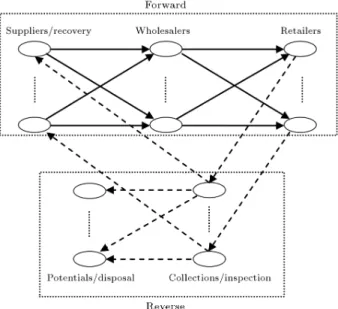
multi-Figure 1. The schema of integrated forward/reverse logistics network.
stage logistics network including supplier/recovery, wholesaler, retailer, collection/inspection and disposal centers. The structure of the IFRLN can be presented in Figure 1. In the forward ow, new products are shipped from supplier/recovery centers to retailer centers directly (from the supplier/recovery centers to the retailer centers) and indirectly (from the sup-plier/recovery centers to the wholesaler centers and then to the retailer centers) to meet the demand of each retailer. In the reverse ow, returned products are collected in collection/inspection centers, and af-ter testing, the recoverable products are shipped to supplier/recovery centers, and scrapped products are shipped to disposal centers.
In this section, a mathematical formulation for the problem is presented. The model has an objective function that minimizes the total purchasing costs of products, transportation costs of products based on the distances, purchasing or hiring costs of vehicles and travel costs of vehicles. The capacity of the sources and depots, and the capacity of the vehicles and limited number of the vehicles are considered in this network. Minimizing costs: Purchasing cost of products, transportation cost of products, purchasing or hiring cost of vehicles, and travel cost of vehicles.
Subject to:
Satisfying demands of all customers; Balancing of ow between nodes; Capacity constraints;
Limited budget for purchasing vehicles;
Assigning only one kind of vehicles for transporting each kind of products;
Non-negativity and binary constraints. 2.1. Indices and sets
i Supplier/recovery center index (i = 1,..., I);
j Wholesaler center index (j = 1,..., J); k Retailer center index (k = 1,..., K); s Collection/inspection center index (s
= 1,..., S);
n Disposal center index (n = 1,..., N); p Product index (p = 1,..., P ); m Vehicle index (m = 1,..., M). 2.2. Decision variables
Ypij Amount of product p transported from
supplier/recovery center i to wholesaler center j;
Vpik Amount of product p transported from
supplier/recovery center i to retailer center k;
Upjk Amount of product p transported from
wholesaler center j to retailer center k; CIpks Amount of return product p
transported from retailer center k to collection/inspection center s; P Rpsi Amount of return product p
transported from collection/inspection center s to supplier/recovery center i; DCpsn Amount of return product p
transported from collection/inspection center s to disposal center n;
B1mpij 1, if vehicle m is used to carry product
p between supplier/recovery center i to wholesaler center j, 0 otherwise; B2mpik 1, if vehicle m is used to carry product
p between supplier/recovery center i to retailer center k, 0 otherwise;
B3mpjk 1, if vehicle m is used to carry product
p between wholesaler center j to retailer center k, 0 otherwise; B4mpks 1, if vehicle m is used to carry
product p between retailer center k to collection/inspection center s, 0 otherwise;
B5mpsi 1, if vehicle m is used to carry product
p between collection/inspection center s to supplier/recovery center i, 0 otherwise;
B6mpsn 1, if vehicle m is used to carry product
p between collection/inspection center s to disposal center n, 0 otherwise;
2.3. Model parameters
dpk Amount of demand for product p by
retailer center k;
bm Maximum budget for purchasing or
hiring vehicle m;
amp Capacity of vehicle m for transporting
product p;
pu1pi Purchasing cost of product p from
supplier/recovery center i;
pu2m Purchasing or hiring cost of vehicle m;
cp Unit transportation cost of product p
along unit distance;
rpk Rate of return of product p of retailer
center k;
ca1pi Supply capacity of supplier/recovery
center i for product p;
ca2pj Delivery capacity of wholesaler center
j for product p; ca3s Delivery capacity of
collection/inspection center s;
ca4n Delivery capacity of disposal center n;
ca5i Recovery capacity of supplier/recovery
center i;
Average disposal fraction 0 1;
; M A large number Pkrpk:dpk 8p;
g1ij Distance between supplier/recovery
center i to wholesaler center j; g2ik Distance between supplier/recovery
center i to retailer center k;
g3jk Distance between wholesaler center j
to retailer center k;
g4ks Distance between retailer center k to
collection/inspection center s;
g5si Distance between collection/inspection
center s to supplier/recovery center i; g6sn Distance between collection/inspection
center s to disposal center n; c1mij Fixed cost of using vehicle
m to carry products between
supplier/recoverycenter i to wholesaler center j;
c2mik Fixed cost of using vehicle m to carry
products between supplier/recovery center i to retailer center k;
c3mjk Fixed cost of using vehicle m to carry
products between wholesaler center j to retailer center k;
c4mks Fixed cost of using vehicle m to carry
products between retailer center k to collection/inspection center s;
c5msi Fixed cost of using vehicle m to carry
products between collection/inspection center s to supplier/recovery center i; c6msn Fixed cost of using vehicle m to carry
products between collection/inspection center s to disposal center n.
2.4. Mathematical formulation
In terms of the above-mentioned notations, the IFRLN design problem can be formulated as follows:
Min
z =X
i
X
j
X
p
(Ypij(pu1pi+ cpg1ij)
+X
m
(pu2m+ c1mij(Ypij=amp))B1mpij)
+X i X k X p
(Vpik(pu1pi+ cpg2ik)
+X
m
(pu2m+ c2mik(Vpik=amp))B2mpik)
+X j X k X p
(Upjkcpg3jk+
X
m
(pu2m
+ c3mjk(Upjk=amp))B3mpjk)
+X k X s X p
(CIpkscpg4ks+
X
m
(pu2m
+ c4mks(CIpks=amp))B4mpks)
+X s X i X p
(P Rpsicpg5si+
X
m
(pu2m
+ c5msi(P Rpsi=amp))B5mpsi)
+X s X n X p
(DCpsncpg6sn+
X
m
(pu2m
+ c6msn(DCpsn=amp))B6mpsn); (1)
S.t. X
j
Upjk+
X
j
Vpik= dpk 8k; p; (2)
X
i
Ypij
X
k
Upjk 8p; j; (3)
X
j
Ypij+
X
k
X
i
Ypij ca2jp 8j; p; (5)
X
k
Upjk ca2jp 8j; p; (6)
X
p
X
k
CIpks ca3s 8s; (7)
X
p
X
s
DCpsn ca4n 8n; (8)
X
p
X
s
P Rpsi ca5i 8i; (9)
X
s
P Rpsi :
X
j
Ypij 8i; p; (10)
X
s
CIpks= rpk:dpk 8p; k; (11)
X
n
DCpsn= :
X
k
CIpks 8p; s; (12)
X
i
P Rpsi= (1 ):
X
k
CIpks 8p; s; (13)
pu2m X p 0 @X i 0 @X j
B1mpij+
X k B2mpik 1 A +X j X k
B3mpjk+
X k X s B4mpks +X s X i
B5mpsi+
X
n
B6mpsn
!!
bm 8m; (14)
Ypij M:
X
m
B1mpij 8i; j; p; (15)
Vpik M:
X
m
B2mpik 8i; k; p; (16)
Upjk M:
X
m
B3mpjk 8j; k; p; (17)
CIpks M:
X
m
B4mpks 8k; s; p; (18)
P Rpsi M:
X
m
B5mpsi 8s; i; p; (19)
DCpsn M:
X
m
B6mpsn 8s; n; p; (20)
X
m
B1mpij 1 8i; j; p; (21)
X
m
B2mpik 1 8i; k; p; (22)
X
m
B3mpjk 1 8j; k; p; (23)
X
m
B4mpks 1 8k; s; p; (24)
X
m
B5mpsi 1 8s; i; p; (25)
X
m
B6mpsn 1 8s; n; p; (26)
B1mpij; B2mpik; B3mpjk; B4mpks; B5mpsi;
B6mpsn2 f0; 1g 8i; j; k; s; n; p; (27)
Ypij; Upjk; Vpik; CIpks; DCpsn; P Rpsi 0
8i; j; k; s; n; p: (28)
In the objective function (1), rst and second terms represent the purchasing cost and transportation cost of products based on the distances, purchasing or hiring cost of vehicles and travel cost of vehicles to carry products from supplier/recovery centers to wholesaler and retailer centers, respectively. 3rd, 4th, 5th and 6th terms represent transportation cost of products based on the distances, purchasing or hiring cost of vehicles and travel cost of vehicles to carry goods and use products between related sources and depots.
Constraint (2) denotes that the total amount of products sent to the retailer centers should be equal to their total demands. Constraint (3) assures that the amount of products sent by each wholesaler center to the retailer center does not exceed the inventory of the warehouse. Constraints (4)-(10) are capacity constraints on facilities. Constraint (11) assures that the ratio of demands as return products are collected in the collection centers. Constraints (12) and (13) assure that in the reverse logistic, a quota of returned products in collection/inspection centers, which are useable, are returned to the supplier centers and others that are unuseable are sent to disposal centers. Constraint (14) represents the constraint of budget for purchasing or hiring vehicles. Constraints (15)-(20) enforce that there should be at least one vehicle to carry products. Constraints (21)-(26) enforce that for each path and each product, only one kind of vehicle should be used. Constraint (27) denotes the binary variables. Con-straint (28) represents the non-negativity restriction of the decision variables.
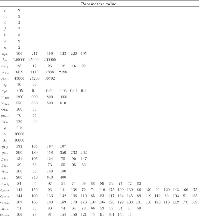
Table 1. Parameters value in a small example. Parameters value
p 2
m 3
i 2
j 2
k 3
s 2
n 2
dpk 100 217 169 123 220 195
bm 150000 250000 200000
amp 23 12 26 18 16 29
pu1pi 3459 4113 1888 2198
pu2m 45000 25200 30792
cp 80 60
rpk 0.05 0.1 0.09 0.06 0.04 0.1
ca1pi 1200 900 800 1000
ca2pj 550 650 500 610
ca3s 100 86
ca4n 70 55
ca5i 120 90
0.2
10000
M 10000
g1ij 132 165 197 107
g2ik 300 180 158 350 232 262
g3jk 131 105 124 75 90 147
g4ks 59 66 73 55 95 80
g5si 100 80 140 180
g6sn 200 840 640 400
c1mij 84 65 97 51 71 69 88 89 59 74 72 82
c2mik 145 150 93 141 138 79 74 119 175 100 130 86 150 90 120 143 166 175
c3mjk 144 100 133 132 106 119 85 83 117 134 145 89 119 112 80 103 91 135
c4mks 109 186 100 169 173 178 107 135 123 172 138 181 116 123 113 112 178 152
c5msi 71 55 80 74 64 70 66 53 59 54 57 59
c6msn 106 78 81 154 156 121 75 91 101 143 71
In order to validate the performance of the model, we present a small example and solve it with LINGO software. The parameters are presented in Table 1 and the variables and objective function are presented in Table 2. It seems that the obtained solution is reasonable.
3. Solution approach
Although the exact algorithms nd the optimal solu-tion, the problems with real size are time consuming. So, the meta-heuristic algorithms are used to nd
the near optimal solution in a reasonable time span. Since the majority of logistics network design problems can be categorized as NP-hard [5], many heuristics and meta-heuristics methods have been developed for solving these problems. In this section, rst, the chromosome representation is described, and then a meta-heuristic algorithm is proposed based on GA and SA to nd the optimal solution in two phases.
3.1. Chromosome representation
In our problem, the solution is represented by a matrix and a vector. In the matrix, the
priority-Table 2. Variables value in a small example. Variables and objective function value
Variable Y122 Y222 B11122 B13222 V112 V113 V212 V213 B21113 B22112 B23212 B23213 U121
Value 100 123 1 1 217 169 220 195 1 1 1 1 100
Variable U221 B32121 B33221 CI111 CI121 CI131 CI211 CI221 CI231 B42111 B42121 B42131 B42211
Value 123 1 1 5 21.7 15.2 7.38 8.8 19.5 1 1 1 1
Variable B42221 B42231 P R112 P R212 B52112 B53212 DC111 DC211 B61111 B63211
Value 1 1 33.53 28.55 1 1 8.38 7.14 1 1
Objective value 0.1665004E+08
based encoding method, proposed by Gen et al. [11], is used. In this approach, solutions are encoded as arrays in which the position of each cell represents the sources and depots, and the value of cells represent the priorities. In the vector, the assigned vehicles to carry the products between the sources and depots are represented in the vector.
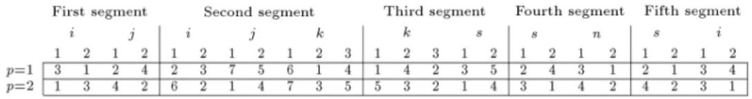
To apply the priority-based encoding method to the problem, for each product type, the priorities are represented in dierent rows. The chromosome consists of ve segments, each of which is related to one echelon of the IFRLN. A typical example of the matrix is shown in Figure 2. The modied priority-based decoding algorithm of a segment is shown in Figure 3.
To decode an IFRLN chromosome, the second segment should be decoded before the rst segment.
Decoding of the second segment contains determining the shipment from supplier/recovery centers to the retailer centers or shipment from wholesaler centers to the retailer centers. The demand of a retailer center would be satised with a supplier/recovery center or a wholesaler center for the minimum cost. Therefore, the Upjk and Vpik could be calculated. After that, the
rst segment should be decoded to determine Ypij. In
this segment, the demand of a wholesaler center, j, for product, p, is what should be sent to the retailer centers (bp;j =PkUpjk). Then, the third, fourth and
fth segments are decoded, respectively, and CIpks,
DCpsn and P Rpsi are calculated. Note that in the
third segment, bp;k = rpk:dpk, in the fourth segment,
bp;s = :PkCIpks and in the fth segment, bp;s =
(1 ):PkCIpks.
Figure 2. The solution representation with the modied priority-based encoding method.
Figure 4. The representation of assignment vector.
In assignment vector, potentially available ve-hicles for transporting all available products in all available routes are represented. The available vehicles for transporting Ypij, Upjk, Vpik, CIpks, DCpsn and
P Rpsi are represented, respectively, in the vector.
A typical example of the vector is shown in Fig-ure 4.
3.2. Operators
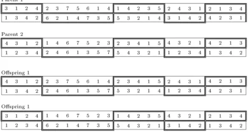
Crossover operator: in the matrix of priorities, segment-based crossover is used. In each row of parents, the corresponding segments are selected alter-nately with equal probability, and are simply swapped to generate osprings (Figure 5).
Mutation operator: in the matrix of priorities, segment-based mutation is used. In each row of selected chromosomes, some segments are selected alternately for mutation. In each selected segment, allele-based mutation is used; two alleles are selected randomly and swapped.
Neighborhood search: in assignment vector, for nding the neighboring solution of the current solution, some alleles are selected randomly from the assignment vector, and their numbers are added to the available vehicles set. Then, some numbers from this set are selected randomly and assigned to the routes indicated by the selected alleles.
3.3. The proposed algorithm
The proposed algorithm consists of two phases. In the rst phase, the optimal routes and amounts of products that must be carried in the routes are determined. Then, in the second phase, the optimal vehicles for transporting the products are determined.
3.3.1. First phase
In this phase, the optimal routes and amounts of prod-ucts which must be carried in the routes are determined using GA. For generating an initial population, random numbers from 1 to each segment size are generated and represented in the segments of the matrices.
In decoding procedure, the costs are determined by variable transportation costs (and purchasing costs) without vehicle costs. Also, for evaluation of chromo-somes, tness function is calculated without vehicles costs. For each solution, if the number of all its routes is more than the number of available vehicles, a very big number, as a penalty function, is added to the tness function to avoid infeasible solutions. The number of available vehicles of kind m is determined by [bm=pu2m].
The roulette wheel selection method is used to select parents. The crossover and mutation operators are used as mentioned. The termination condition is reaching to maximum generation number and a feasible solution, in which the entire routes is less than or equal to the total number of vehicles.
3.3.2. Second phase
After determining the optimal routes and amounts of products, which must be carried in the rst phase, in the next phase, the kind of vehicles for transporting the products between the selected sources and depots are determined. The number of optimal routes is less than or equal to the available vehicles. The SA algorithm is used to determine the optimal assignment of vehicles to the routes. For generating an initial solution, the available vehicles for transporting Ypij,
Upjk, Vpik, CIpks, DCpsn and P Rpsi are selected
randomly from the available vehicles set, and are represented respectively in the vector.
In this phase, the tness function is only calcu-lated by the costs of using vehicles for transporting
Figure 6. Proposed algorithm for the IFRLN.
amounts of products that has been determined in the rst phase.
After determining the optimal tness function values in the rst and second phases, the results are summarized to show the true tness function. The proposed algorithm for the IFRLN is summarized in Figure 6.
4. Computational results
In order to validate the performance of the algorithm, we generate several instances. The mathematical model of IFRLN is coded in LINGO optimization software, and the proposed meta-heuristic algorithm
is coded in MATLAB on a computer with 4.0 GB Ram and 2.66 GHz processor. The Response Surface Methodology (RSM) is used to determine the optimal parameters of the algorithm. The model solutions and the meta-heuristic solutions are compared on the problem instances.
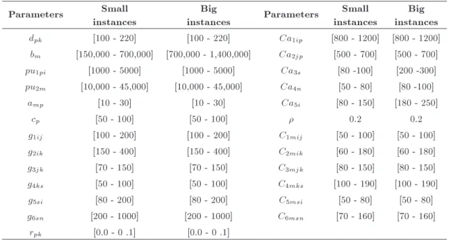
4.1. Data generation
Here, ftheen instances are dened that can be char-acterized by the number of products (np), between 2
and 7, vehicles (nm) between 2 and 6, supplier/recovery
centers (ni) between 2 and 9, wholesaler centers (nj)
between 2 and 11, retailer centers (nk) between 2 and
Table 3. Parameters range in the test problems.
Parameters Small
instances
Big
instances Parameters
Small instances
Big instances dpk [100 - 220] [100 - 220] Ca1ip [800 - 1200] [800 - 1200]
bm [150,000 - 700,000] [700,000 - 1,400,000] Ca2jp [500 - 700] [500 - 700]
pu1pi [1000 - 5000] [1000 - 5000] Ca3s [80 -100] [200 -300]
pu2m [10,000 - 45,000] [10,000 - 45,000] Ca4n [50 - 80] [80 -100]
amp [10 - 30] [10 - 30] Ca5i [80 - 150] [180 - 250]
cp [50 - 100] [50 - 100] 0.2 0.2
g1ij [100 - 200] [100 - 200] C1mij [50 - 100] [50 - 100]
g2ik [150 - 400] [150 - 400] C2mik [60 - 180] [60 - 180]
g3jk [70 - 150] [70 - 150] C3mjk [80 - 150] [80 - 150]
g4ks [50 - 100] [50 - 100] C4mks [100 - 190] [100 - 190]
g5si [80 - 200] [80 - 200] C5msi [50 - 80] [50 - 80]
g6sn [200 - 1000] [200 - 1000] C6msn [70 - 160] [70 - 160]
rpk [0.0 - 0 .1] [0.0 - 0 .1]
and disposal centers (nn) between 2 and 7. The data
required in the IFRLN problem are generated randomly as shown in Table 3.
4.2. Parameters tuning of the proposed algorithm
The parameters employed in algorithms should be se-lected properly to obtain a satisfactory solution quality in an acceptable time span. The RSM method is used to determine the optimal parameters of the algorithm. This is a technique for determining and representing the cause-and-eect relationship between true mean responses and input control variables inuencing the responses as a multi-dimensional hyper surface [14]. This method has four stages. In the rst stage, the independent parameters and their levels are deter-mined. Some points (scenarios) are selected using these levels. In the second stage, the proposed algorithm is applied to several test problems, using these points. The results are normalized with relative percentage deviation (RPD) criteria (Eq. (29)). After collecting the data, the third stage is the prediction of the model equation and obtaining the response surface as a function of the independent variables (parameters and their interactions). Signicant variables and coecient of each variable are found, so the regression equation is determined. The fourth stage is determination of the optimum points of the equation.
RP D = Algsol minsol
minsol : (29)
The crossover rate (pc), mutation rate (pm), initial
temperature (t0), iterations at a specic temperature
(k) and cooling rate (a) are the ve important factors
Table 4. Levels of proposed algorithm parameters. Parameter Lower
level
Middle value
Upper level
pc 0.5 0.6 0.7
pm 0.1 0.15 0.2
t0 30 45 60
k 60 90 120
a 0.94 0.96 0.98
aecting the proposed algorithm. So, eects of these parameters and their interactions are studied as input variables in the optimization procedure. For each parameter, the levels of parameters are dened as shown in Table 4.
The 25 2 points, using two-level factorial design,
4 central points and 2 5 axial points are selected. For each point, each problem instance is carried out 5 times, and average value of the objective function values and the processing times are recorded. These results are normalized by RPD criteria, and the average values for each point are calculated. The two regression models of the objective function and the processing time are determined using minitab14 software. The two regression models are optimized as a bi-objective problem, using a bi-objective technique and lingo9 software. The rst equation is optimized, then, its solution is considered as a constraint in optimizing the second equation.
The results show that the models were highly signicant with p values = 0.000. The optimal values are pc = 0:58, pm = 0:17, t0 = 25, k = 144 and
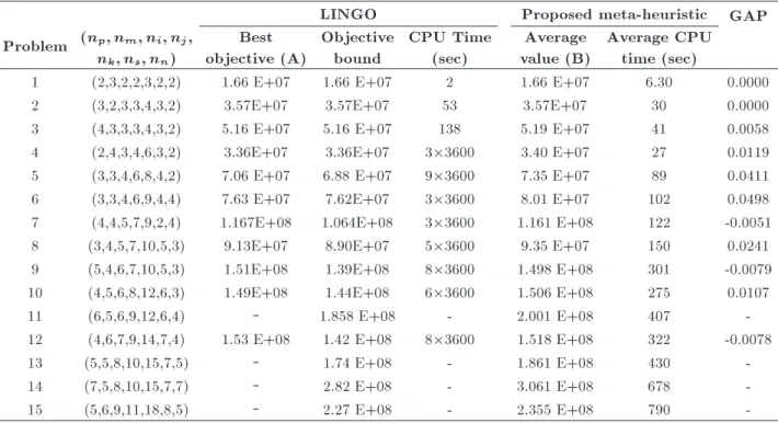
Table 5. Results of LINGO and the proposed algorithm solutions.
LINGO Proposed meta-heuristic GAP
Problem (np; nm; ni; nj;
nk; ns; nn)
Best objective (A)
Objective bound
CPU Time (sec)
Average value (B)
Average CPU time (sec)
1 (2,3,2,2,3,2,2) 1.66 E+07 1.66 E+07 2 1.66 E+07 6.30 0.0000
2 (3,2,3,3,4,3,2) 3.57E+07 3.57E+07 53 3.57E+07 30 0.0000
3 (4,3,3,3,4,3,2) 5.16 E+07 5.16 E+07 138 5.19 E+07 41 0.0058
4 (2,4,3,4,6,3,2) 3.36E+07 3.36E+07 33600 3.40 E+07 27 0.0119
5 (3,3,4,6,8,4,2) 7.06 E+07 6.88 E+07 93600 7.35 E+07 89 0.0411
6 (3,3,4,6,9,4,4) 7.63 E+07 7.62E+07 33600 8.01 E+07 102 0.0498
7 (4,4,5,7,9,2,4) 1.167E+08 1.064E+08 33600 1.161 E+08 122 -0.0051
8 (3,4,5,7,10,5,3) 9.13E+07 8.90E+07 53600 9.35 E+07 150 0.0241
9 (5,4,6,7,10,5,3) 1.51E+08 1.39E+08 83600 1.498 E+08 301 -0.0079 10 (4,5,6,8,12,6,3) 1.49E+08 1.44E+08 63600 1.506 E+08 275 0.0107
11 (6,5,6,9,12,6,4)
1.858 E+08 - 2.001 E+08 407-12 (4,6,7,9,14,7,4) 1.53 E+08 1.42 E+08 83600 1.518 E+08 322 -0.0078
13 (5,5,8,10,15,7,5)
1.74 E+08 - 1.861 E+08 430-14 (7,5,8,10,15,7,7)
2.82 E+08 - 3.061 E+08 678-15 (5,6,9,11,18,8,5)
2.27 E+08 - 2.355 E+08 790-Also in the rst phase, the population size is selected 100. The maximum generation is selected 100 for small instances and 200 for large instances. 4.3. Numerical results
The proposed algorithm is executed ve times for each problem. The average values and LINGO results are shown in Table 5. A quality criterion, GAP, is dened to show the relative dierence between the LINGO and proposed algorithm solutions. Let A and B denote the best objective value, using the LINGO and the average objective values of the proposed meta-heuristic algorithm, respectively. Now dene the GAP as:
GAP =B AR : (30)
The lower the value of this metric, the better the solution quality.
As shown in Table 5, the proposed algorithm nds the near optimal solutions in less computational time. In small size problems, the proposed algorithm has found optimal solution similar to LINGO (problems 1 and 2). But when the problem size increases, LINGO cannot nd proper solution in reasonable time, while the proposed algorithm nds near-the-objective-bound solutions in less computational time. For the problems 5-10 and 12, LINGO cannot nd the optimal solutions within 600 second, and instead of optimal solutions, the best feasible solution is given as comparison. In the large scale problems, LINGO cannot nd any solution in an acceptable time span, but the proposed algorithm nds the solution near the objective bound of the
problem in a reasonable time span (problems 11 and 13-15). The proposed algorithm in comparison with LINGO only nds slightly worse solutions in a few problems. GAP values do not exceed 5% for these problems. In the problems 7, 9 and 12, the proposed algorithm in comparison with LINGO nds better solution in shorter computational time (GAP < 0). In the large size problems, LINGO cannot nd any solution in an acceptable time span, but the proposed algorithm nds the solution near the objective bound of the problem, in a reasonable time span.
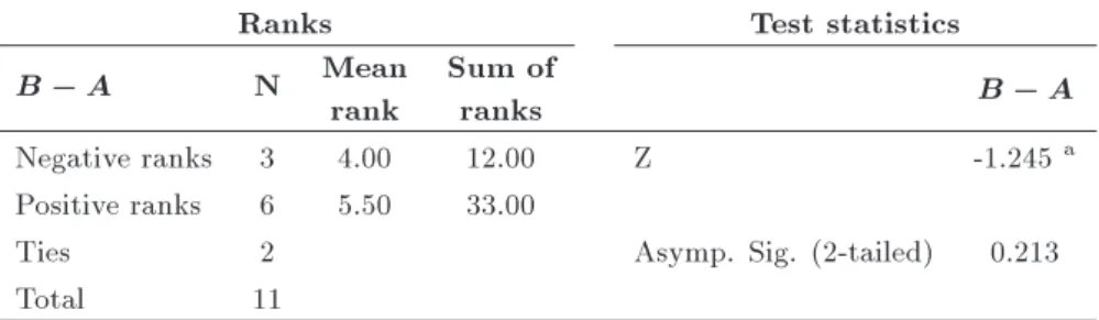
For verication of the algorithm, appropriate statistical tests can be used to test the signicant dierence between two sets A and B, as follows:
(
H0: A= B
H1: A6= B (31)
Nonparametric tests should be used due to the non-parametric characteristics of the data. Wilcoxon signed rank test is one of these tests that is used for paired comparisons. This test is employed using SPSS 16 soft-ware. The result is shown in Table 6. Signicant level, 0.213, shows that there are no reasons for rejecting zero hypotheses with a 95% condence level. So, there is no signicant dierence between the performance of the algorithm and using LINGO for solving the model.
The convergence speed of the rst phase of the proposed algorithm is depicted in Figure 7. It is obvious that tness function value decreases steeply and the proposed algorithm reaches the optimal value of the rst phase after 25 generations.
Table 6. Result of Wilcoxon test on responses.
Ranks Test statistics
B A N Mean
rank
Sum of
ranks B A
Negative ranks 3 4.00 12.00 Z -1.245a
Positive ranks 6 5.50 33.00
Ties 2 Asymp. Sig. (2-tailed) 0.213
Total 11
a: Based on negative ranks.
Figure 7. Convergence curve of the proposed algorithm.
5. Conclusions
In this paper, a designing and transportation planning in a multi-stage multi-product supply chain network is examined. Decision makers need to determine the optimal routes and vehicles when there is a limited bud-get for hiring vehicles. We considered the Integrated Forward/Reverse Logistics Network (IFRLN) problem and formulated it as a Mixed Integer Nonlinear Pro-gramming model (MINLP) to minimize the total costs of purchasing the products, hiring the vehicles and transportation.
The problem is NP-hard, so we developed a hybrid meta-heuristic algorithm based on pb-GA and SA algorithm in two phases to nd optimal solution. The solution is represented by a matrix and a vector. In the matrix, the position of each cell represents the sources and depots, and the value in cells represents the priorities. Each row of the matrix is corresponding to a product type. In the assignment vector, the assigned vehicles are represented to carry products between the sources and depots. The algorithm is composed of two phases. In the rst phase, the amount of products to be carried between the sources and depots are determined. Then, in the second phase, the vehicles for transporting products are determined.
Response Surface Methodology (RSM) was used to set the eective parameters of the algorithms. Sev-eral problems were generated and solved with LINGO
optimization software and the proposed meta-heuristic algorithm. The results showed that the proposed algorithm can nd the solution in less computational time. The results of Wilcoxon test showed that there is no signicant dierence between the objective function values of the algorithm and using LINGO for solving the problem.
For future research, other objectives can be used in this logistic network. Scheduling problems can be considered. Satisfying customers' demands on time will increase service level of the supply chain. The network responsiveness also can be used to satisfy the customers. Holding cost can be added to the objective function, and minimized.
GRASP (Gready Randomized Adaptive Search Procedure) algorithm can be used to generate the initial population, instead of generating it randomly. So, the algorithm will have three phases. Other metaheuristic algorithms can be developed to solve the problem, and then the algorithms can be compared from convergence to the optimal solution. In the second phase, other neighborhood search algorithms like local search and tabu search can be applied.
References
1. Hitchcock, F.L. \The distribution of a product from several sources to numerous localities", Journal of Math. Phys., 20, pp. 224-230 (1941).
2. Tilanus, B. \Introduction to information system in logistics and transportation", In: Tilanus B, Ed., Information Systems in Logistics and Transportation, Elsevier, Amsterdam, pp. 7-16 (1997).
3. Fleischmann, M., Beullens, P., Bloemhof-ruwaard, J.M. and Wassenhove, L. \The impact of product recovery on logistics network design", Production and Operations Management, 10, pp. 156-173 (2001).
4. Lee, D.H. and Dong, M. \Dynamic network design for reverse logistics operations under uncertainty", Transportation Research Part E, 45, pp. 61-71 (2009).
5. Pishvaee, M.S., Farahani, R.Z. and Dulaert, W. \A memetic algorithm for bi-objective integrated forward/ reverse logistics network design", Computer & Opera-tion Research, 37, pp. 1100-1112 (2010).
6. Farahani, R.Z. and Elahipanah, M. \A genetic al-gorithm to optimize the total cost and service level
for JIT distribution in a supply chain", International Journal of Production Economics, 111, pp. 229-243 (2008).
7. Zegordi, S.H. and Beheshti Nia, M.A. \A multi-population genetic algorithm for transportation scheduling", Transportation Research Part E, 45, pp. 946-959 (2009).
8. Michalewicz, Z., Vignaux, G.A. and Hobbs, M. \A non-standard genetic algorithm for the nonlinear transportation problem", ORSA Journal on Comput-ing, 3(4), pp. 307-316 (1991).
9. Li, Y.Z., Gen, M. and Ida, K. \Improved genetic algo-rithm for solving multi-objective solid transportation problem with fuzzy number", International Journal of Fuzzy Theory Systems, 4(3), pp. 220-229 (1998).
10. Gen, M. and Cheng, R.W., Genetic Algorithms and Engineering Optimization, Wiley, New York (2000).
11. Gen, M., Altiparmak, F. and Lin, L. \A genetic algorithm for two-stage transportation problem using priority-based encoding", OR Spectrum, 28, pp. 337-354 (2006).
12. Lee, J.E., Gen, M. and Rhee, K.G. \Network model and optimization of reverse logistics by hybrid genetic algorithm", Computers & Industrial Engineering, 56, pp. 951-964 (2009).
13. Lin, L., Gen, M. and Wang, X. \Integrated multistage logistics network design by using hybrid evolutionary algorithm", Computers & Industrial Engineering, 56, pp. 854-873 (2009).
14. Gunaraj, V. and Murugan, N. \Application of response surface methodology for predicting weld bead quality in submerged arc welding of pipes", Journal of Mate-rials Processing Technology, 88, pp. 266-275 (1999).
Biographies
Esmaeil Mehdizadeh is currently Assistant Pro-fessor at the Department of Industrial Engineering, Islamic Azad University, Qazvin Branch, Iran. He
received his PhD degree in Industrial Engineering from Islamic Azad University, Science and Research Branch, Tehran, in 2009. His research interests are in the areas of operation research such as production planning, scheduling and meta-heuristic methods. He has several papers in journals and conference proceedings.
Fariborz Afrabandpei is currently Production Plan-ner in Ilam Gas Treating Company, National Iranian Gas Company, Ilam, Iran. He received his MSc degree in Industrial Engineering from Industrial Engineering Department, Islamic Azad University, Qazvin Branch, Iran in 2012. His research interests are in the areas of operation researches such as production planning and scheduling. He has studied supply chain management and bi-objective methods.
Somayeh Mohaselafshar received her BS degree in Applied Mathematics from Tabriz University, Tabriz, Iran and her MSc degree in Industrial Engineering from Mazandaran University of Science and Technology, Babol, Iran in 2011. Her research interests are in the areas of operation research such as production planning, scheduling and meta-heuristic methods. She has studied supply chain management, manufacturing cells, job scheduling on machines and bi-objective methods. She is a member of Tabriz municipality. Behrouz Afshar-Nadja is currently Assistant Pro-fessor and Graduate Programs Manager of Indus-trial Engineering at Islamic Azad University, Qazvin Branch, Qazvin, Iran. He received his PhD degree in Industrial Engineering at Sharif University of Tech-nology, in 2008. His research interests are the project scheduling, Inventory and production planning. Cur-rently, he is working on modeling and solution methods including exact procedures, meta-heuristic algorithms and articial intelligence techniques regarding discrete optimization problems in reality.