Sharif University of Technology
Scientia IranicaTransactions E: Industrial Engineering www.scientiairanica.com
Solving the redundancy allocation problem of
k-out-of-n with non-exponential repairable components
using optimization via simulation approach
P. Azimi
, M. Hemmati and A. Chambari
Faculty of Industrial and Mechanical Engineering, Qazvin Branch, Islamic Azad University, Qazvin, Iran. Received 26 May 2015; received in revised form 30 September 2015; accepted 5 September 2016
KEYWORDS Redundancy allocation problem; k-out-of-n systems; Meta-heuristic algorithms;
Simulation methods; Enterprise Dynamic (ED) software.
Abstract.In this article, a new model and a novel solving method are provided to address the non-exponential redundancy allocation problem in series-parallel k-out-of-n systems with repairable components based on Optimization Via Simulation (OVS) technique. Despite the previous studies, in this model, the failure and repair times of each component were considered to have non-negative exponential distributions. This assumption makes the model closer to the reality where the majority of used components have greater chance to face a breakdown in comparison to new ones. The main objective of this research is the optimization of Mean Time to the First Failure (MTTFF) of the system via allocating the best redundant components to each subsystem. Since this objective function of the problem could not be explicitly mentioned, the simulation technique was applied to model the problem, and dierent experimental designs were produced using DOE methods. To solve the problem, some meta-Heuristic Algorithms were integrated with the simulation method. Several experiments were carried out to test the proposed approach; as a result, the proposed approach is much more real than previous models, and the near optimum solutions are also promising.
© 2017 Sharif University of Technology. All rights reserved.
1. Introduction
The increase in system reliability has been one of the most appealing areas for the engineers and designers, and the utilization of redundant components is one of the common approaches in the development of the systems. Each system is formed by putting dierent components together wherein their way of relation with each other depends on their function in the system. Dierent kinds of the system structures could be sys-tems with parallel, series, series-parallel, parallel-series components, and bridge network structures [1]. In this
*. Corresponding author. Tel./Fax: +982833665275 E-mail addresses: [email protected] (P. Azimi); [email protected] (M. Hemmati); [email protected] (A. Chambari)
paper, series-parallel structures are used; consequently, it is one of those system structures designed by allo-cating redundant components in parallel to the compo-nents of a system with series structure [2]. Reliability is the probability of proper function of system in a certain time interval, and the reliability of the whole system is a combination of reliability of its individual compo-nents. Two approaches are proposed for increasing the reliability of system. The rst approach is to increase the reliability of system components; the second is to use the redundant components in addition to the main components in parallel [3]. Due to economic and technological limitations, the best and most ecient method of increasing system reliability is the second approach by using the redundant components with the main components. For this reason, this approach is used in this article as well [4]. Redundancy strategies
are categorized into active and standby strategies. In an active redundancy strategy, it is assumed that all of the redundant components are implemented together from time zero, whereas in the standby strategy, only the components operate. Hence, the redundant components are idle until the active component fails. Thus, whenever a component in operation fails, one of the redundant components should be switched on. In this paper, the active redundancy is considered. After the rst article by Fye et al. [5], in which they studied the redundancy allocation problem in series-parallel systems, a great number of researchers have tried to develop this knowledge. The investigations of Coelho [6], Zou et al. [7], Ramirez-Marquez and Coit [8], Nahas et al. [9], Safaei et al. [10], Liang and Chen [11], Ha and Kuo [12], Soltani et al. [13], Liang et al. [14], Juang et al. [15], Zhang et al. [16], and Chambari et al. [17] are of those investigations into the redundancy allocation problem in series-parallel systems. For more information about the redundancy allocation problems, readers are referred to a work by Soltani [18].
With a glance at the trend of the studies in redundancy allocation problem, it is clearly seen that this problem has not been addressed in the repairable systems. The lack of investigations into the redun-dancy allocation problem in series-parallel systems with repairable components and subsystems by Kuo and Wan [19], Guedenko and Ushakov [20], Elegbede and Adjallah [21], and Ying-Shen et al. [22] is com-pensated after some nished research works in the literature of redundancy allocation problem. Since the structure of the system has a signicant eect on system reliability, the reparability or non-reparability of system components or subsystems is another issue aecting the proper function of a system in its oper-ating duration. The system reparability means that it is possible to restart the system by the required repairs of failures. Whenever a system is repairable, \availability" is used instead of reliability. Availability is the percentage of the time during which a repairable system appropriately does the dened tasks [19]. In this paper, reparability components are considered.
For the multi-objective redundancy allocation problem, Chambari et al. [23], for non-repairable components, considered a large series-parallel system with two objectives: maximization of system reliability and minimization of cost. Garg et al. [24] managed to maximize system reliability and minimize cost by Particle Swarm Optimization (PSO) in a series-parallel system. Zoulfaghari et al. [25] formulated bi-objective redundancy allocation problem with two objectives, including maximization of the system availability and minimization of cost of the system considering repara-bility and non-repararepara-bility components. Furthermore, Li and Lin [26] considered three-objective models,
whose objectives include reliability, total cost, and total weight.
Since a dierent word other than reliability is dened as a functional parameter of the system for repairable systems, the other notions regarding the system function are also dierent in repairable systems. Mean Time To the Failure (MTTF) or survivability in non-repairable systems shows the mean durability of system lifetime, while the components of a repairable system are repairable and the system could restart after repair, and the MTTF is the mean time of system failure for the rst time (MTTFF) [27].
The aim of this manuscript is to represent a bi-objective model developed for the series-parallel system to allocate redundant components in systems to repairable components in order to maximize MTTFF of the system and minimize system cost under the constraints of total cost, weigh of the system, and sum of components within the system. The redun-dancy allocation problem is the non-linear polynomial optimization problem which is of NP-hard class [28]. It has been addressed by dierent methods and with the extension of solution space, the absolute solutions in solving these problems are inecient; the meta-heuristic approaches have been preferred instead in recent years. Then, since the proposed model belongs to an NP-hard class of optimization problems, an eective Multi-Population Genetic Algorithm (MPGA) is implemented to solve the model.
The rest of the paper is organized as follows. Section 2 denes multi-objective optimization more precisely and describes the problem denition and basic assumptions in Section 3. Section 4 develops the pro-posed methods for solving the reliability optimization problem. Section 5 describes computational results and provides analysis of the results for a set of test problems. Finally, Section 6 concludes the paper and all remarks.
2. Multi-objective optimization
Multi-Objective Optimization Problem (MOOP) refers to the problems in which two or more objectives must be optimized simultaneously. Often, such objectives are in conict with each other and are expressed in dif-ferent units. Because of their nature, the nal solution to MOOP is not a single one but a set of solution known as Pareto-solutions [29,30]. When such solutions are represented in the objective function space, the graph produced is called the front or the Pareto-optimal set. A general formulation of a MOOP consists of a number of objectives with a number of inequality and equality constraints. The problem can be mathe-matically written as minff1(x); f2(x); ; fv(x)g
sub-ject to gl(x) 0; l = 1; 2; ; L and hk(x) = 0;
fv(x) is the ith objective function, and gl(x) and hk(x)
are constraints vectors. In the function set, some of the objectives are often in conict with others; some have to be minimized, while others are to be maximized. The constraints limit feasible region X, and any point x 2 X is categorized as feasible solutions. There is rarely a situation in which all fv(x) function values
have an optimum in X at common point x. Therefore, in the absence of preference information, solutions to multi-objective problems are compared using the no-tion of Pareto dominance. In a minimizano-tion problem for all objectives, solution x1 dominates solution x2
(also written as x1 > x2), if and only if the two
following conditions are true:
x1is no worse than x2in all objectives, i.e. fv(x1)
fv(x2); 9v 2 f1; 2; ; V g;
x1is strictly better than x2for at least one objective,
i.e. fv(x1) < fv(x2); 9v 2 f1; 2; ; V g.
Then, a solution is said to be Pareto-optimal if it is not dominated by any other possible solution, as described above. Thus, the Pareto-optimal solutions to a multi-objective optimization problem form the Pareto-front or Pareto-optimal set [31].
3. Problem denition
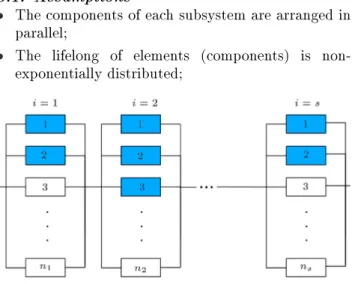
In this article, k-out-of-n system containing S inde-pendent subsystems, as in Figure 1, is considered. Since this structure is more realistic, it is the most important and the most utilized structure in dierent studies [32]. In this structure, a system is arranged with S subsystems beside each other; in each subsystem ni (i = 1; 2; ; S), dierent components are arranged
in parallel. There are dierent types of component choices per subsystem, and the components within the same subsystem are of the same type.
3.1. Assumptions
The components of each subsystem are arranged in parallel;
The lifelong of elements (components) is non-exponentially distributed;
Figure 1. The structure of a k-out-of-n system containing s independent sub-systems.
The components are repairable and the repair rate of elements is also non-exponential;
Mixture of components is allowed within a subsys-tem;
The components allocated to each subsystem are of the same type;
A certain number of components are utilized within each subsystem;
There is one repairman able to repair all the com-ponents.
3.2. Mathematical model of the problem
According to the assumptions, the applied symbols, indices, and mathematical models including objective function and the constraints of the problem are as follows:
3.2.1. Symbols, indices, and variables of the problem i Index of subsystem
j Index of component choice used for subsystems i
xij Number of selected components of type
j for subsystem i
ij Failure rate of component of type j for
subsystem i
ij Repair rate of component of type j for
subsystem i
S Number of subsystems
ni Number of components allocated to
subsystem i
cij Cost of component j available for
subsystem i
wij Weight of component j available for
subsystem i
Ws Weight of the system
Ni Upper bound for ni
Ns Maximum number of components used
in the whole system
yij Binary variable to choose/not choose
one component type for the subsystem i
M A big number 3.2.2. Mathematical model
max Z = minfMTTFSig; (1)
min Cs= S
X
i=1 ni
X
j=1
s.t.
S
X
i=1 ni
X
j=1
wij xij Ws; (3)
ni
X
j=1
yij=1; 0xijNi:yij 8i=1; ; S; (4)
S
X
i=1 ni
X
j=1
xij Ns; (5)
ki ni
X
j=1
xij Ni 8i = 1; ; S; (6)
yij 2 f0; 1gki; xij 0; int; (7)
where:
MTTFSi = f(xij; ij; ij):
Eq. (1) is the main objective function or Mean MTTFF of the system. The second objective function of the problem is based on the minimization of the total cost of the system in Eq. (2); Eq. (3) is the system weight constraint; constraints required to choose only one component type are provided in Eq. (4); Eq. (5) is the constraint of number of components of the whole system; Eq. (6) is the constraint of lower and upper bounds for the number of components allocated to each subsystem; for the proper function of each subsystem, it is required that, at least, ki out of ni components
operates. And nally, the constraint of components' type and their extents is provided in Eq. (7).
The aim of this article is to increase MTTFF of a series-parallel system. In this system, there are components arranged in parallel in each subsystem, and a subsystem operates in spite of failures and repairs until all the components fail. This system with its series subsystems fails for the rst time, i.e. the rst failure occurs whenever one of the subsystems completely fails [8]. Hence, mean time of the rst failure of the system is the mean time within which one of the subsystems completely fails. Therefore, the increase of mean time of the rst failure of the system is the minimum value of the mean failure of each subsystem. The algorithm for the calculation of MTTFF of a subsystem with parallel and reparable components is provided in [33].
4. Methods for reliability optimization
The methods for reliability optimization are classied into three main categories of exact, approximate, heuristic and meta-heuristic. These are explained as follows [4,18]:
Exact methods: In these methods, the optimal solution is calculated for the reliability optimization problems. Rate of the computations of the exact method exponentially increases according to the increase of the problem quantity. Some of the exact methods are dynamic programming, gradient method, linear programming, and integer program-ming;
Approximate method: In these methods, the model of the problem is approximated due to the complexity of the models, and the optimal solution to the approximate model is calculated using the exact methods. Some of the important approximate methods are the geometric programming, Lagrange multiplier method, random search and lexicographic method;
Heuristic and meta-heuristic methods: Con-sidering the long duration of computation, the heuristic and meta-heuristic methods are proposed. These methods provide a near optimal solution in a proper computational time.
4.1. The proposed solving methods 4.1.1. The Multi-Population Genetic Algorithm
(MPGA)
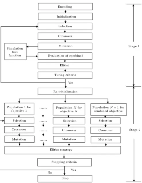
The two-stage approach, which we call MPGA, is illustrated in Figure 2. In the rst stage, the GA evolves based on the combined objective. The solutions at the end of the rst stage are rearranged and divided into subpopulations, then they start to evolve separately. The steps of each stage are described in the following subsection. Essentially, this approach uses a modication of Multi-Objective Genetic Algorithm (MOGA) in stage one and a modication of Vector Evaluated Genetic Algorithm (VEGA) in stage two. The general pseudo-code of the proposed MPGA is described in Figure 2.
Encoding
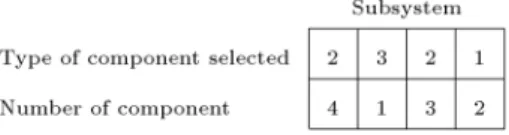
The rst step in running the Genetic Algorithm is to represent the solution or design the chromosome. The chromosomes are so designed to estimate the main limitations of the problem as much as possible. The chromosome designed in this study is a T N matrix where T represents the type and number of selected components, and N is the number of subsystems. Each column represents a subsystem, and the value of each cell in the rst row represents the type; in the second row, the value of each cell represents the number of components in the relevant subsystem.
For example, Figure 3 shows the layout of a sys-tem with four subsyssys-tems, where in the rst subsyssys-tem, there are four components of type two; in the second subsystem, there is one component of type three; in the third subsystem, there are three components of type
Figure 2. The general pseudo-code of the proposed MPGA.
Figure 3. Encoding solution as a chromosome representation.
two; in the fourth subsystem, there are two components of type one.
Initialization
In this article, dierent populations are generated instead of using only the initial population and running the steps of genetic algorithm on it. The chromosome structure is the same as in all of these populations, but each population could have its own steps of selection, generation, and mutation; after some generations, we exchange the chromosomes within them by Elitism Algorithms. Since the eciency of dierent models of Genetic Algorithm heavily depends on data types, the proposed method minimizes the risk of exposure to local minimum due to its possibility to use various methods in each population.
Selection
Selection is an operation to select two parent strings for generating new ospring. Let Xi
t be the ith
solution (I between 1 and population size) in the tth generation, and f(xi
t) be the performance measure of
solution Xi
t. Each solution Xti is selected as a parent
string according to the selection probability P (xi t). The
following method is used: P (xi
t) = [f w
t f(xit)]2
PN
k=1[ftw f(xkt)]2
; (8)
where fw
t is the worst value of objective at generation
t.
Crossover
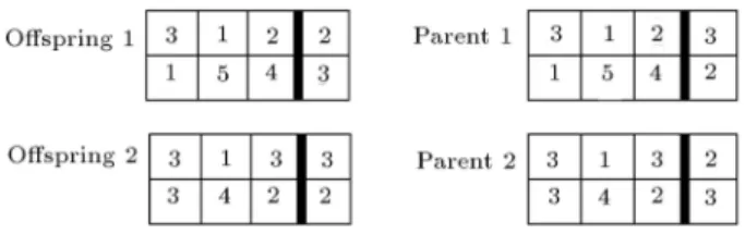
For crossover operation, we follow steps below consid-ering the condition of feasibility of the generated o-springs:
1. The rst chromosome of the population is selected;
2. Generate a random number r between 0 and 1;
3. If r < Pc, then choose that algorithm for the
Figure 4. An example of the crossover process to ne new solutions.
4. Now, pair the selected chromosomes randomly; generate a random number of \cross point" per chromosome in the range of f1; ; Ng, where N is the number of subsystems;
5. Copy the bits of 1 through cross point in the chromosome of the rst parent directly into the genes of the rst o-spring;
6. The bits of cross point+1 through N of the second parent are transited to the rst o-spring according to their arrangement in the second parent;
7. Repeat steps 6 and 7 for the generation of the second o-spring;
8. Repeat the above steps to generate the other o-spring chromosomes.
The crossover process is shown in Figure 4 schemati-cally.
Mutation
The most important function of mutation operator is to avoid the convergence and local optimum and searching in intact spaces of the problem. The task of mutation of a chromosome is to change its genes, and it has dierent methods depending on the type of coding. We follow the steps below concerning the mutation on the chromosomes:
1. The rst chromosome in the population is selected;
2. Generate a random number r between 0 and 1;
3. If r < Pm, then the chromosome is mutated, i.e.
one of the genes of the component type or the number of components is selected and replaced with another value being randomly and feasibly gener-ated. Figure 5 illustrates this operator graphically. Evaluation of the main objective function A series-parallel system fails for the rst time when one of the subsystems fails, i.e. if each subsystem of the system fails rst, it results in the failure of the whole system. Hence, in order to calculate the MTTFF of the
Figure 5. Example of the mutation process to avoid local optimums.
system, it is required to simulate the MTTFF of each subsystem, and the MTTFF value of the subsystem which has the earliest failure time is considered as the MTTFF of the whole system. Since all the relations and equations for calculating the MTTFF of a system are possible by failure probabilities and exponential repair by mathematical and statistical analyses; it is not possible by any kind of repair or analysis other than non-exponential repair, and in this way, the simulation approach is applied to calculate this value. It should be noted that the tness of each chromosome is equal to their mean tness in n times of simulation of that chromosome. Therefore, we are able to calculate the tness rate of each chromosome without any unrealistic assumption.
Evaluation of the combined objective
One of the most famous methods of multi-objective optimization (MOOP) is \weighted aggregation". In this method, a linear combination of objective func-tions with non-negative dierent weights is used to form \aggregated function" as below:
F (x) =Xm
i=1
wifi(x) m
X
i=1
wi= 1; wi 0: (9)
In the above formula, F (x) is aggregated function, and wi is lth non-negative weight related to lth objective
function. There are dierent methods for aggregating objective function and producing aggregated function F (x). The best method to estimate aggregation of functions is \Dynamic Weighted Aggregation" method (DWA), because this method shows better ability to estimate concave Pareto-fronts. This method is dened for two objective functions as below (it can be general-ized easily to more than two-objective functions):
(w1(t); w2(t)) = (j sin(2t=R)j; 1 w1(t)); (10)
where t is tth sub-population (t = 1; 2; ; Ns) and R = 200.
MOOPs are usually solved by scalarization (it means converting the problem with multiple objectives into a single objective or a family of single objec-tive optimization problems). The major trouble of weighting method is the need for scalarizing multiple objectives in sum weighting, and in this regard, we employ one of the most widely used multi-objective methods called Min-Max. In Min-Max approach, we use the idea of minimizing the distance of every solution from the best possible solution f. In other way, if
fi(x) is the ith objective function and fi is the best
available solution for fi(x), then the quantity of f
will be f = (f
1; f1; ; fm)T. So, the following
function is minimized subject to the constraint of the problem:
min " m
X
i=1
fi(x) fi
f i
p#1 p
;
s.t. X 2 S;
1 p 1: (11)
Exponent p shows various ways for measuring the dis-tance. The most widely applied values of p are 1 for the simplest formulation and 2 for the Euclidean distance, Andersson [34]. The major challenge in this approach is to nd the value of p that will maximize the satisfaction of Decision-Makers (DM). Another shortcoming of this method is that there is only one output, and DM has to accept it as a nal solution. Thus, in this phase, through mixing the weighting and Min-Max method, two problems will be solved, one of which is the mono-solution of Min-Max, and the other is the problem of scalarzing in weighting method. Consequently, there would be two-objective functions dened by:
w
f1(x) f1
f 1
p
+(1 w)
f2(x) f2
f 2
p1 p
; (12)
where f1(x) and f2(x) indicate each individual minima
of each respective objective function, and 0 < w < 1. w denotes the weight (or relative importance) of a number of setups and the usage rate. In this paper, p value is determined as 1. Because the scales of the objectives are dierent, the normalization process has been applied to objective values of this method. Note that all the examples solved here have used 10 dierent seeds for every algorithm, and the minimum solution in all runs is f for each objective. These are
substituted in Eq. (13). Elitist
The best solution of each objective and the best one of the combined objective function are preserved in each generation. For each generation, if the best solution is worse than the preserved one, a randomly selected string will be replaced with the preserved.
Turning criterion
After a certain number of generations, the algorithm switches to the next stage. In stage 2, the populations of the solution from stage 1 will be rearranged based on their performance of each objective.
Re-initialization
Assume N objectives to be optimized, as discussed above, the solutions from the rst stage are rear-ranged and N + 1 sub-populations will be created and evolved separately. The rst stage through Nth sub-populations is for N objectives, and (N + 1)th subpopulation is for the combined objective.
Selection, Crossover, and Mutation
The same selection, crossover, and mutation proce-dures used in Stage 1 are applied to each subpopu-lation.
Elitist strategy
Although each sub-population evolves separately, the elitist strategy searches for the best solution to each objective and combined objective across all subpopu-lations. N + 1 solutions will be stored and will replace the worst solution of each objective and the combined objective.
Stopping criteria
A test run indicates that the algorithm does not show signicant improvement after 2,000 generations. However, to consider the error due to the randomness and have more promising results, a larger generation number should be used as the stopping criteria. In addition, most literature reviews have used 3,000 generations to stop the algorithm. Therefore, 3,000 generations are used in this study as stopping criteria. A ow chart of the proposed MPGA is depicted in Figure 6.
4.1.2. Weighted sum Multi-Objective Genetic Algorithm (WMOGA)
One of the most famous methods in multi-objective optimization is \weighted aggregation". The two objectives are usually formulated in a weighted sum approach. The details of the proposed WMOGA are presented in Figure 7.
4.1.3. Non-dominated Sorting Genetic Algorithm II (NSGA-II)
As a well-known Multi-Objective Evolutionary Algo-rithm (MOEA), the NSGA-II has been the most widely used and has been proven to do well on various real-world application problems [35]. The pseudo-code of NSGA-II is presented in Algorithm 1 in Figure 8. We used NSGA-II in our research, since there have been many investigations ensuring that NSGA-II can often converge to Pareto-optimal set, and the obtained solu-tions can often spread well over the Pareto-optimal set. NSGA-II takes the fast non-dominated-sort mechanism to ensure the well convergence, shown in Algorithm 2, Figure 8. For details of NSGA-II, one can refer to [36]. The general pseudo-code of the NSGA-II is described in Figure 8.
5. Computational results
In order to conduct the experiment, we implement the proposed algorithms in Matlab 7.8 software, ED 8.1 to simulate the problem. All computations are on a PC with Intel Pentium 4, 1.67 GHz processor, 4 GByte memories with windows 7 Professional Operating System.
Figure 6. A two-stage Multi-Population Genetic Algorithm (MPGA).
Test problems: The experiments were implemented over 30 test problems. For all experiments, the following assumptions were considered:
Data generation: Also, in this article, a series of experiments are designed where the following values are considered for the variety of distributions:
The component type one has exponential distribu-tion: for the failure (mean value) in the range of (0.06, 0.25) and for the repair value in the range of (0.033, 0.167) are considered, respectively;
The component type two has Erlang distribution: for the failure of the components, the value of in the range of (0.3, 0.9) and = 2; for the repair, the value of in the range of (0.1, 0.6) and = 2 are considered, respectively;
The component type three has Weibull distribution: for the failure of the components, the value of in the range of (0.5, 0.9) and = 0:5 and for the repair, the value of in the range of (0.1, 0.5) and = 0:5 are considered, respectively.
In order to explain the eciency of the proposed algorithms, the illustrative examples are designed with 30 experiments. The number of subsystems in the problem is 5, 15, and 20 subsystems based on which the random problems are produced in small, medium, and large sizes. For each size, 10 sample problems are generated. In these problems, the maximum number of the components in each subsystem is between 5-10, the minimum number of components for each subsystem is between 2-4, the volume and cost of each component are between 200-300 and 100-500, and the maximum volume available for the system is between 9000-13000.
Figure 7. The pseudo-code of the WMOGA.
Figure 8. The pseudo-code of the NSGA-II.
Comparator algorithms: Performance of the de-veloped MPGA was compared with two Meta heuristics developed for the multi-objective redundancy alloca-tion problem, discussed in this paper in a set of problems.
5.1. Parameters settings
This subsection tries to nd the optimal parameter setting in the algorithms. There are several parameters that may inuence the performance of the algorithms. For example, the larger population size may nd better solution quality but cost higher computational expense.
It should be noted that changing these parameters may result in dierent outcomes than those achieved in this research. When the number of populations is larger, it may have better diversity. However, it may also be a trade-o to cut the number of generations. Moreover, the crossover and mutation operator is also considered, because it may oer better solution quality. The parameters' setting of algorithms is indicated in Table 1.
5.2. Performance measures
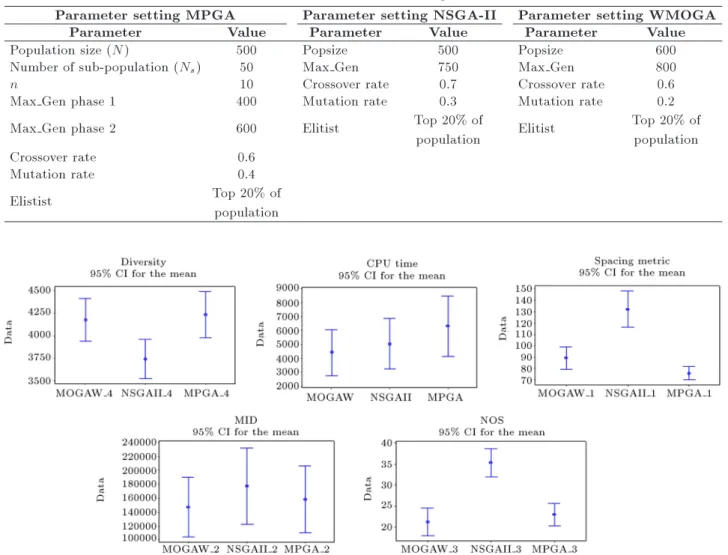
Table 1. Parameter setting.
Parameter setting MPGA Parameter setting NSGA-II Parameter setting WMOGA
Parameter Value Parameter Value Parameter Value
Population size (N) 500 Popsize 500 Popsize 600
Number of sub-population (Ns) 50 Max Gen 750 Max Gen 800
n 10 Crossover rate 0.7 Crossover rate 0.6
Max Gen phase 1 400 Mutation rate 0.3 Mutation rate 0.2
Max Gen phase 2 600 Elitist Top 20% of
population Elitist
Top 20% of population
Crossover rate 0.6
Mutation rate 0.4
Elistist Top 20% of
population
Figure 9. Comparability of MPGA in comparison with NSGA-II and WMOGA on diversity, CPU time, MID, spacing, and NOS metrics.
ve standard metrics of multi-objective algorithms are applied as follows:
Diversity: Measures the extension of the Pareto front in which bigger value is better [23];
Spacing: Measures the standard deviation of the distances among solutions of the Pareto front in which smaller value is better [23];
Mean Ideal Distance (MID): Measures the conver-gence rate of the Pareto front to a certain point (0, 0) in which smaller value is better [23];
Number Of found Solutions (NOS): Counts the number of the Pareto solutions in Pareto optimal front in which bigger value is better;
The computational (CPU) time of running the algorithms to reach near optimum solutions.
The experiments are implemented on 30 test problems. Furthermore, to eliminate uncertainties of the solutions obtained, each problem is used three
times under dierent random environments. Then, the averages of these three runs are treated as the ultimate responses. Then, we compare the proposed MPGA algorithm with WMOGA and NSGA-II as the most applicable Pareto-based MOEAs in the test prob-lem to demonstrate the performance of the proposed algorithm to solve the multi-objective optimization problems.
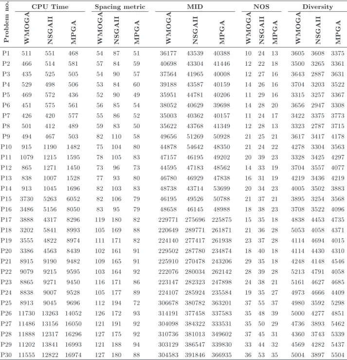
To evaluate the performance of the proposed MPGA, Table 2 reports the multi-objective metrics' amounts on 30 test problems, in which \NAS" shows that the algorithm cannot nd Pareto front in the reported time.
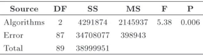
The algorithms are statistically compared based on the properties of their obtained solutions via the analysis of variance (ANOVA) test. These outputs are reported in Tables 3 to 7 in terms of dened metrics. In order to clarify our statistical results, interval-plots are represented in Figure 9.
Based on the statistical outputs in Tables 3 and 6 along with Figure 9, NSGA-II shows better
Table 2. Evaluation of non-dominated solution for algorithms grouped by problem size and index type.
Problem
no. CPU Time Spacing metric MID NOS Diversity
WMOGA NSGAI
I
MPGA WMOGA NSGAI
I
MPGA WMOGA NSGAI
I
MPGA WMOGA NSGAI
I
MPGA WMOGA NSGAI
I
MPGA
P1 511 551 468 54 87 51 36177 43539 40388 10 24 13 3605 3608 3375
P2 466 514 581 57 84 59 40698 43304 41446 12 22 18 3500 3265 3361
P3 435 525 505 54 90 57 37564 41965 40008 12 27 16 3643 2887 3631
P4 529 498 506 53 84 60 39188 43587 40159 14 26 16 3704 3203 3522
P5 469 572 436 52 90 49 35951 44781 40206 11 29 16 3315 3257 3367
P6 451 575 561 56 85 54 38052 40629 39698 14 28 20 3656 2947 3308
P7 426 420 577 55 86 52 35003 40362 40157 11 24 17 3422 3375 3773
P8 501 412 489 59 83 50 35622 43768 41349 12 28 13 3323 2787 3715
P9 494 467 503 82 110 58 49656 51269 50928 21 25 21 3617 3417 4178
P10 915 1190 1482 75 104 80 44878 54642 48350 21 24 22 4278 3304 3563 P11 1079 1215 1595 78 105 83 47157 46195 49202 20 39 23 3328 3425 4297 P12 865 1271 1450 73 96 73 44595 47183 48562 14 33 19 3704 3557 4077 P13 838 1007 1528 77 93 80 46780 46929 47838 16 31 19 4219 3436 4219 P14 913 1045 1696 82 103 83 48738 43714 53699 20 34 23 4005 3502 3883 P15 3730 5263 6052 82 106 79 46195 49526 50788 21 37 21 3895 3254 3568 P16 3486 5156 8050 83 95 79 48658 46145 48988 18 38 23 3708 3522 4096 P17 3888 4317 8296 119 180 82 229771 275696 225875 15 35 18 4838 4453 4735 P18 3202 5841 8993 105 169 88 220649 289771 261871 21 36 28 5053 4058 4371 P19 3555 4822 8974 111 171 82 224140 277417 261938 23 37 28 4114 4694 4015 P20 3386 4563 8439 102 161 91 229502 287780 234874 18 40 18 4114 4430 4310 P21 8915 9190 9482 109 165 91 225910 270478 243206 29 35 18 4248 4148 4546 P22 9079 9215 9595 103 164 92 222076 280034 262142 28 39 28 5213 4791 4058 P23 8865 9271 9450 116 171 86 223147 282323 247898 24 38 21 5161 4627 4685 P24 8838 9007 9528 105 177 89 224107 285924 235584 19 35 27 4973 4666 4409 P25 8913 9045 9696 112 194 72 306678 380782 363201 37 55 37 4980 3592 5298 P26 11730 13263 14052 126 172 93 314191 377458 337583 35 48 39 5000 4277 4851 P27 11486 13156 16050 121 191 92 304098 384322 333531 35 50 29 4736 3893 5462 P28 11888 12317 16296 127 175 92 310736 381013 349602 37 45 31 4360 3743 5339 P29 11202 13841 16993 121 188 94 303129 386547 339830 33 44 32 4569 4282 5437 P30 11555 12822 16974 127 180 88 304583 391846 366935 36 53 35 5004 3897 5504
performances in terms of NOS, while WMOGA has a better performance in terms of CPU time.
Moreover, Tables 4 to 7 along with Figure 9 show the comparability of MPGA in comparison with NSGA-II and WMOGA on MID, spacing, and diver-sity metrics, in which the algorithms have no sig-nicant dierences and statistically work the same. It is required to be mentioned that this conclusion is conrmed at 95% condence level. Based on the outputs in Table 2, there is the increasing of size of problems in test problems 22 and 30; in test problem 30, NSGA-II and WMOGA cannot nd Pareto front,
Table 3. Analysis of variance for the time metric.
Source DF SS MS F P
Algorithms 2 55606000 278030 1.09 0.340 Error 87 221143724 254188
Total 89 226704324
Table 4. Analysis of variance for the spacing metric.
Source DF SS MS F P
Algorithms 2 51401 25701 28.00 0.000
Error 87 79855 918
Table 5. Analysis of variance for the MID metric.
Source DF SS MS F P
Algorithms 2 139856556 699282 0.40 0.669 Error 87 1.508E+12 173386
Total 89 1.525E+12
Table 6. Analysis of variance for the NOS metric.
Source DF SS MS F P
Algorithms 2 3529.9 1764.9 25.98 0.000 Error 87 5910.6 67.9
Total 89 9440.5
Table 7. Analysis of variance for the diversity metric.
Source DF SS MS F P
Algorithms 2 4291874 2145937 5.38 0.006 Error 87 34708077 398943
Total 89 38999951
respectively. However, in these large sizes, MPGA can nd Pareto front. The MPGA algorithm performs better performance in the terms and CPUT metric. These features conclude robustness of the proposed MPGA in large-sized problems in the area of multi-objective optimization problems.
6. Conclusions
In this article, a new method is provided to model and solve the Redundancy Allocation Problem in the k-out-of-n series-parallel systems with non-exponential repairable components based on OVS technique. A bi-objective function was used to model the system. The rst one was optimizing the Mean Time To the First Failure (MTTFF) of the system, and the second one was minimizing the total costs. The components are assumed to have non-exponential breakdowns and repair times, which are the main contributions of this research. A model with non-exponential components is closer to the reality where the memoryless property is rare to be found among the components. In general, the used components have shorter expected life time in comparison to new ones. Also, we have no practical reasons to assume exponential distributions for the components of repair times. When the stochastic events, such as the failures and repair times, are non-exponential, the MTFFF function cannot be written explicitly. This is the simulation technique which enables us to model and solve the model, where all stochastic events with any kind of distribution function could be modeled easily. In order to demonstrate appli-cability of the proposed solving algorithm (MPGA), the multi-objective reliability problems were applied. The proposed algorithm was able to improve the quality of
the obtained solutions by taking the specic advantages of the multi-population Genetic Algorithm and also using the simulation techniques.
The results show the capability of the MPGA algorithm to solve the multi-objective problems. To justify the proposed algorithm, NSGA-II and WMOGA algorithms have been implemented to evaluate the performance of the proposed MPGA. The results show the eciency of MPGA in the large-size problems. For future research, one may compare the proposed MPGA with other multi-objective algorithms (e.g., MOPSO or MOTS) in various optimization problems.
References
1. Kapur, K.C. and Lamberson, L.R., Reliability in Engineering Design, New York, John Wiley & Sons (1987).
2. Tekiner-Mogulkoc, H. and Coit, D.W. \System relia-bility optimization considering uncertainty: minimiza-tion of the coecient of variaminimiza-tion for series-parallel systems", Reliability, IEEE Transactions on, 60(3), pp. 667-674 (2011).
3. Garg, H. \An ecient biogeography based optimiza-tion algorithm for solving reliability optimizaoptimiza-tion prob-lems", Swarm and Evolutionary Computation, 24, pp. 1-10 (2015).
4. Kuo, W. and Prasad, V.R. \An annotated overview of system-reliability optimization", IEEE Transaction on Reliability, 2, pp. 176-187 (2000).
5. Fye, D.E., Hines, W.W. and Lee, N.K. \System reliability allocation and a computational algorithm", IEEE Transaction on Reliability, pp. 64-69 (1968).
6. Coelho, L.D.S. \Reliability-redundancy optimization by means of a chaotic dierential evolution approach", Chaos, Solitons and Fractal, pp. 594-602 (2009).
7. Zou, D., Gao, L., Li, S. and Wu, J. \An eective global harmony search algorithm for reliability problems", Expert Systems with Applications, 38(4), pp. 4642-4648 (2011).
8. Ramirez-Marquez, J.E. and Coit, D.W. \A heuristic for solving the redundancy allocation problem for multi-state series-parallel system", Reliability Engi-neering and System Safety, pp. 314-349 (2004).
9. Nahas, N., Nourelfath, M. and Ait-Kadi, D. \Coupling ant colony and the degraded ceiling algorithm for the redundancy allocation problem of series-parallel systems", Reliability Engineering and System Safety, pp. 211-222 (2007).
10. Safaei, N., Tavakkoli-Moghaddam, R. and Kiassat, C. \Annealing-based particle swarm optimization to solve the redundant reliability problem with multiple component choices", Applied Soft Computing, 12(11), pp. 3462-3471 (2012).
11. Liang, Y.C. and Chen, Y.C. \Redundancy allocation of series parallel systems using a variable neighborhood
search algorithm", Reliability Engineering and System Safety, pp. 323-331 (2007).
12. Ha, C. and Kuo, W. \Reliability redundancy alloca-tion: An improved realization for non-convex nonlinear programming problems", European Journal of Opera-tion Research, pp. 24-38 (2006).
13. Soltani, R., Sadjadi, S.J. and Togh, A.A. \A model to enhance the reliability of the serial parallel systems with component mixing", Applied Mathematical Mod-elling, 38, pp. 1064-1076 (2013).
14. Liang, Y.C., Lo, M.H. and Chen, Y.C. \Variable neigh-borhood search for redundancy allocation problems", IMA Journal of Management Mathematics, pp. 135-155 (2007).
15. Juang, Y.S., Lin, S.S. and Kao, H.P. \A knowledge management system for series-parallel availability opti-mization and design", Expert System and Applications, pp. 181-193 (2008).
16. Zhang, E., Wu, Y. and Chen, Q. \A practical approach for solving multi-objective reliability redundancy al-location problems using extended bare-bones particle swarm optimization", Reliability Engineering & Sys-tem Safety, 127, pp. 65-76 (2014).
17. Chambari, A., Naja, A.A., Rahmati, S.H.A. and Karimi, A. \An ecient simulated annealing algorithm for the redundancy allocation problem with a choice of redundancy strategies", Reliability Engineering & System Safety, 119, pp. 158-164 (2013).
18. Soltani, R. \Reliability optimization of binary state non-repairable systems: A state of the art survey", International Journal of Industrial Engineering Com-putations, 5(3), pp. 339-364 (2014).
19. Kuo, W. and Wan, R. \Recent advances in optimal reliability allocation", IEEE Transaction on System, Man and Cybernetics-Part a: System and Humans, pp. 143-156 (2007).
20. Guedenko, B. and Ushakov, I., Probabilistic Reliability Engineering, A Wiley-Interscience Publication, New York (1995).
21. Elegbede, C. and Adjallah, K. \Availability allocation to repairable systems with genetic algorithms: A multi-objective formulation", Reliability Engineering and System Safety, 82, pp. 319-330 (2003).
22. Ying-Shen, J., Shui-Shun, L. and Hsing-Pei, K. \A knowledge management system for series-parallel avail-ability optimization and design", Expert Systems with Applications, 34, pp. 181-193 (2008).
23. Chambari, A., Rahmati, S.H.A. and Naja, A.A. \A bi-objective model to optimize reliability and cost of system with a choice of redundancy strategies", Computers & Industrial Engineering, 63(1), pp. 109-119 (2012).
24. Garg, H., Rani, M., Sharma, S.P. and Vishwakarma, Y. \Bi-objective optimization of the reliability-redundancy allocation problem for series-parallel sys-tem", Journal of Manufacturing Systems, 33(2), pp. 353-367 (2014).
25. Zoulfaghari, H., Hamadani, A.Z. and AboueiArdakan, M.A. \Bi-objective redundancy allocation problem for a system with mixed repairable and non-repairable components", ISA Transactions, pp. 17-24 (2014).
26. Li, Z., Liao, H. and Coit, D.W. \A two-stage approach for multi-objective decision making with applications to system reliability optimization", Reliability Engi-neering and System Safety, 94, pp. 1585-1592 (2009).
27. Lai, C-D. and Lin, G.D. \Mean time to failure of systems with dependent components", Applied Mathe-matics and Computation, 246(1), pp. 103-111 (2014).
28. Naja, A.A., Karimi, H., Chambari, A. and Azimi, F. \Two metaheuristics for solving the reliability re-dundancy allocation problem to maximize mean time to failure of a series-parallel system", Scientia Iranica, 20(3), pp. 832-838 (2013).
29. Garg, H. and Sharma, S.P. \Multi-objective reliability-redundancy allocation problem using particle swarm optimization", Computers & Industrial Engineering, 64, pp. 247-255 (2013).
30. Khalili-Damghani, K., Abtahi, A.R. and Tavana, M. \A new multi-objective particle swarm optimization method for solving reliability redundancy allocation problems", Reliability Engineering & System Safety, 111, pp. 58-75 (2013).
31. Deb, K., Agrawal, S., Pratap, A. and Meyarivan, T. \A fast elitist non-dominated sorting genetic algorithm for multi-objective optimization: NSGA- II", In Proceed-ings of the Parallel Problem Solving from Nature VI (PPSN-VI) Conference, pp. 849-858 (2000).
32. Coit, D.W. and Liu, J. \System reliability optimization with k-out-of-n subsystems", International Journal of Reliability, Quality and Safety Engineering, 7(2), pp. 129-142 (2000).
33. Amiri, M. and Ghassemi-Tari, F. \A methodology for analyzing the transient availability and survivability of a system with repairable components", Applied Mathematics and computation, pp. 300-307 (2007).
34. Andersson, J. \A survey of multi-objective optimiza-tion in engineering design", In Technical Report LiTH-IKP-R-1097, Department of Mechanical Engineering, Linkoping University, Linkoping, Sweden (2000).
35. CoelloCoello, C.A., Van Veldhuizen, D.A. and Lamont, G.B., Evolutionary Algorithms for Solving Multi Objec-tive Problems, Kluwer Academic Publishers (2002).
36. Srinivas, N. and Deb, K. \Multi objective optimization using non-dominated sorting in genetic algorithms", Evolutionary Computation, MIT Press Journals, 2(3), pp. 221-248 (1994).
Biographies
Parham Azimi was born in 1974 in Tehran. He received his PhD degree in Industrial Engineering in Sharif University of Technology. He has been a university tutor at the Faculty of Industrial and
Mechanical Engineering at Qazvin Islamic University since 2004. His research interests are optimization via simulation, graph labeling problems, and simulation modeling.
Mojtaba Hemmati received his BS and MS degrees in Industrial Engineering from Qazvin Islamic Azad University, Iran, where he is currently a PhD student. His research interests include applications of operations research in redundancy allocation problems, queuing system, and more specically, modeling and solution
methods including exact procedures, simulation meth-ods and articial intelligence techniques.
Amirhossein Chambari received his MS degree in Industrial Engineering from Islamic Azad Univer-sity, Qazvin, Iran, in 2010, where he is currently a PhD student. He currently works as purchase ex-pert of the oil Co., Tehran, Iran. His research inter-ests include reliability engineering, facility location-allocation, simulation methods, and articial intelli-gence techniques.