Vol. 17, No. 1, pp. 71{80 c
Sharif University of Technology, June 2010
Classifying Hypnotizable Groups Using
EEG Weighted Regional Frequency
G. Baghdadi
1and A. Motie Nasrabadi
1;Abstract. Determination of hypnotizability is important, before prescribing any hypnotic treatment. Existing methods for measuring the level of hypnotic susceptibility are subjective, with some problems. In this study, a feature based on EEG weighted regional frequency was introduced, which can characterize the level of the subject's hypnotizability objectively. The ability of this feature for making a signicant dierence between three hypnotizable groups at the end of hypnotic suggestion was shown using statistical analyses. This feature was calculated based on the empirical mode decomposition method and the Hilbert transform. The EEG signals that were used in this study were recorded during hypnotic suggestion from 32 subjects. A K-nearest neighborhood-based classier was designed for classication of the hypnotizable groups. The performance of the classier was validated using the leave-one-out method, which showed the mean error of 3.13% in determination of the subject's hypnotic susceptibility level. This evaluation and obtaining the error were done by comparing the new method's results with the score of hypnotizability that was determined for each subject, using the subjective Waterloo-Stanford criterion. The new method, as opposed to common subjective clinical methods, represents a real time and objective procedure for determining hypnotic susceptibility.
Keywords: Hypnosis; Hypnotizability; Empirical mode decomposition; Hilbert transform; Classication; K-nearest neighborhood.
INTRODUCTION
In recent years, much research has been devoted to processing EEG signals that can be recorded from the brain in dierent situations such as sleep, anesthesia and hypnosis. Hypnosis is a trance-like state of mind. The purpose of hypnosis is to help the subject gain more control over his behavior, emotions or physical well-being. Hypnotherapists say that hypnosis creates a state of deep relaxation and quiets the mind. When a person is hypnotized, he can concentrate intensely on a specic thought, memory, feeling or sensation, while blocking out distractions, and this can be used to change his behavior and, thereby, improve his health and well-being. However, these changes can only be done when the subject is more open than usual to suggestion. In other words, the best eect of hypnotherapy is on subjects who are more hypnoti-zable. Hypnotizability is the ability to experience a
1. Department of Biomedical Engineering, Shahed University, Tehran, P.O. Box 3319118651, Iran.
*. Corresponding author. E-mail: [email protected] Received 29 May 2009; received in revised form 7 October 2009; accepted 8 December 2009
hypnotic trance. People vary in their ability to go into a trance at will and on purpose. Nowadays, the current method for determination of hypnotizability is the use of dierent standard tests that measure how well a subject conforms to the behavior of a classically hypnotized person [1-7]. Using the results of these tests, some people are found to be markedly more hypnotizable. There are dierent international tests, such as the Stanford Hypnotic Susceptibility Scale (SHSS) [8,9], the Hypnotic Induction Prole (HIP) [6] and the Waterloo-Stanford Group Scale of hypnotic susceptibility (WSGS) [2-5], which were designed in order to characterize the hypnotic susceptibility of a subject based on dierent questions and activities that a hypnotizer wants a subject to answer and perform. These standard clinical tests are subjective, so, they have some problems. As an example, clinical and subjective evaluations take time and are boring, which sometimes makes the subject tired and reduces the level of hypnotic trance. Also, sometimes the subjects try to cheat the hypnotherapist, so he has to investigate the reactions of the subject to the tests in order to obtain a real hypnotizability level. Because of these problems, researchers try to nd an
objective method for determining the hypnotizability level. In this way, they try to investigate the eect of hypnosis on dierent biological signals [10-18]. In this study, we focus on hypnosis and its eects on the EEG signal, in order to determine the level of hypnotizability.
Several studies have been directed to the iden-tication of the hypnosis eect on EEG signals. Ini-tial studies [19-21] suggested that highly hypnotiz-able people produced more EEG alpha under resting conditions than low-hypnotizable people. However, Evans [22] did not show this dierence and sug-gested that previous results were biased by demand characteristics, and Dumas [23] suggested that the alpha-hypnotizability relationship resulted from biased subject selection [23]. Perlini and Spanos [24], in their critical review of alpha and hypnotizability, concluded that there is little support for an alpha-hypnotizability relationship. Gran et al. [25] showed that following a standardized hypnotic induction, low susceptible participants displayed an increase in theta activity, whereas high-susceptible participants displayed a de-crease.
Ray [26], using fractal dimensionality measures, reported that highly hypnotizable individuals display underlying brain patterns associated with imagery, whereas low hypnotizable individuals show patterns consistent with cognitive activity.
Abootalebi et al. [27] investigated and found the relation between hypnotizability and higher order spectra of EEG signals. The ndings of these studies have not been consistently replicated either. One explanation is that perhaps the subject's personal pref-erences, and the hypnotic techniques used in dierent studies vary widely; by the fact that brain activity diers in hypnosis depending on the nature of the suggestions. Nasrabadi [28] represents a method for estimating the hypnotizability score based on EEG feature extraction.
Horton et al. [29] performed the rst MRI study to report dierences in brain structure size between low and highly hypnotizable, healthy, right-handed young adults. They imported that highly hypnotizable subjects had a signicantly larger rostrum (a corpus callosum area involved in the allocation of attention and transfer of information between prefrontal cortices) than low hypnotizable subjects.
Lee et al. [30] investigated the correlation between HIP-induction scores and the scaling exponent of DFA, but he found no relation between this feature and hypnotizability.
Baghdadi & Nasrabadi [31] showed that some EEG fractal features have a signicant relationship with the nal depth of the hypnosis or hypnotizability level.
Behbahani and Nasrabadi [32] propose a method
for classifying hypnotizable groups, based on the fuzzy similarity index of hypnosis EEG signals. Behbahani reported that based on a fuzzy similarity index feature we can classify the highly hypnotizable subjects from other subjects with high accuracy.
The mentioned studies, except [26,31], tried to nd the eect of hypnosis on dierent brain wave features, not to classify the subjects into dierent hypnotizable groups. In this way, the studies are con-tinued in order to nd an objective general method for classifying subjects into more hypnotic susceptibility levels, such as very low, low, medium, high and very high.
This paper oers a promising method for clas-sifying three hypnotizable groups (Low, medium and high) using calculation of the weighted regional fre-quencies based on an Empirical Mode Decomposition method (EMD) and Hilbert Transformation (HT). A combination of these two algorithms, which is called the Hilbert Huang Transform (HHT), was used for analyz-ing EEG signals duranalyz-ing dierent brain activities [33-37]. Empirical mode decomposition is a new method for analyzing nonlinear and non-stationary data. By this method, any complicated data set can be decomposed into a nite and often small number of intrinsic mode functions that admit well-behaved Hilbert transforms. This decomposition method is adaptive and, therefore, highly ecient. Since the decomposition is based on the local characteristic time scale of the data, it is applicable to nonlinear and non-stationary processes. The EMD method was initially proposed for the study of ocean waves [38], and found immediate applications in biomedical engineering [39,40]. In this study, the EMD method was implemented in a study of the hypnotizability of dierent subjects and an eort was made to nd out if there is a signicant dierence between three hypnotizable groups (low, medium and high) using a weighted regional frequency instead of common and earlier subjective clinical methods, such as WSGS.
MATERIALS AND METHODS Data and Subjects
The data includes EEG signals that were recorded from 32 right-handed men during hypnosis. EEG data were recorded from 19 channels and were sampled with 256 Hz based on a 10-20 system of electrode placement. Hypnosis induction was done by playing a recorded sound on a tape, so, the method and time of the hypnosis induction were the same for all subjects. This tape was based on the Waterloo-Stanford criterion [2-5]. An EEG was recorded for 15 minutes during the hypnosis induction. In order to evaluate and compare the new method's results with a subjective
Table 1. Demographic and clinical characteristics of subjects.
Gender Male
Number of hypnosis sessions 3-6 times
Physical features of subjects before recording
No high physical activity Enough relaxation Right handed Duration of hypnosis 15 mins
Time of recording Afternoon (about 4 to 8 o'clock) Score of hypnotizability in Waterloo-Stanford criterion 12 to 52
Number of low hypnotizable subjects 4 Number of medium hypnotizable subjects 18 Number of high hypnotizable subjects 10
method, a score of hypnotizability was determined for each subject based on the subjective Waterloo-Stanford criterion. The WSGS scores are between 12-60. Based on these scores, the subjects divided into three groups, low (WSGS scores are between 12 and 22), medium (WSGS scores are between 23 and 41) and high (WSGS scores are between 42 and 60). Table 1 shows the demographic and clinical characteristics of subjects.
Empirical Mode Decomposition (EMD)
Huang et al. [38] have introduced the EMD method for nonlinear and nonstationary signal analysis. The general idea of this method is the sifting process to decompose any given signal into its intrinsic oscilla-tions. With the EMD approach, the basic functions themselves are nonlinear, which can be derived directly from the data. Hence, the analysis is adaptive. The adaptive basis is called the Intrinsic Mode Function (IMF) and this method decomposes a time series into a nite and often small number of IMFs each of which must satisfy the following denition:
1. Number of extreme and number of zero-crossings must dier at most by one.
2. At any point, the mean value of the upper and lower envelope is zero.
The IMFs, xi(t), of a signal y(t), is found by the
following loop:
1. Compute the mean of upper and lower envelopes of signal, m(t),
2. Subtract from the signal to obtain zi(t) = y(t)
m(t).
3. Check if zi(t) is an IMF, then, zi(t) is the rst IMF
of y(t). If it is not an IMF, zi(t) is treated as the
original signal and steps 1 to 3 are repeated;
4. Separating zi(t) from y(t), we get yi(t) = y(t)
zi(t). yi(t) is treated as the original data and, by
repeating the above processes, the second IMF of y(t) could be obtained [41-43].
The second step is applying the Hilbert transform to each IMF, in order to compute the instantaneous frequency and amplitude at each time [38,44]. X(t) in the following equation is the Hilbert transform of Y (t).
X(t) = Hilbert TranformfY (t)g = 1
1
Z
1
Y (t) t t0dt0:
(1) Using Equation 1, instantaneous frequency, If(t), and instantaneous amplitude, a(t), are dened as [38,44,45]:
a(t) =pY2(t) + X2(t); (2)
(
If(t) = d(t)2dt
(t) = arctanhX(T )Y (T )i: (3)
Weighted Instantaneous and Regional Frequency
Equations 2 and 3 give the frequencies and their ampli-tudes that make a signal in each time. Investigating the time-frequency-amplitude spectrum of a signal shows that a number of frequencies have larger amplitude, and this subject oers that these frequencies are more dominant in each time. However, a simple average of all obtained frequencies in each time does not consider the larger eect of the dominant frequencies. This problem can be solved by considering a larger weight for the dominant frequencies in calculating the average frequency in each time. In this study, the weight of each instantaneous frequency, Ifj(t), is
the instantaneous amplitude of this frequency, aj(t),
divided by the summation of all instantaneous fre-quency amplitudes (see Equation 4). Therefore, the weight of the instantaneous frequencies that have the larger amplitude is greater than of those with lower amplitudes.
W IF (t) =Xn
j=1
aj(t)Ifj(t)= n
X
j=1
aj(t); (4)
where n is the number of the IMFs of a signal that is recorded from one of the brain channels. Ifj(t) and aj(t) is the series of the estimated
in-stantaneous frequency and amplitude for each IMF [44]. W IF (t) is a series of weighted instantaneous frequencies. In this study, we used the average of W IF (t) in dierent time windows of the hypnosis EEG, so we have used a weighted regional frequency instead of an instantaneous frequency (see Equa-tion 5).
RF =t
0+T
X
t=t0
W IF (t): (5)
Therefore, RF is the average of W IF s in a time window whose duration is T . In this paper, the ability of this feature in dierent brain channels is investigated in order to classify the hypnotizable groups.
Statistical Analysis and Area Under ROC Curve
Before designing and using any classier, it was tested whether or not a feature based on a weighted regional frequency can make a signicant dierence between three hypnotizable groups. This investigation was performed using some statistical analyses, such as ANOVA [46] and MANOVA [47,48]. The normality of the data was investigated before performing the analyses. ANOVA was used when one feature was employed for making a dierence between three hypno-tizable groups and MANOVA was used in a situation where the ability of the simultaneous usage of dierent features was investigated. The MANOVA can also give a linear combination of the dierent features that make the largest separation between groups. Calculation of the coecients of this linear combination was done by maximizing the F ratio:
F = W~ T P
bW~
~
WTP ~W : (6)
This ratio represents the between groups variability, b, with respect to within the groups variability, .
This means that when ~W is an eigenvector of 1 b,
the separation will be equal to the corresponding eigenvalue. Therefore, the coecients of the linear combination maximize the ratio of between-groups to within-groups variance.
For more condence about the results of the statistical analyses, we calculated the area under the ROC curve, abbreviated as AUC. The ROC curve is a two-dimensional depiction of the classier performance. The two axes of this graph represent tradeos between errors (false positives) and benets (true positives) that a classier makes between two classes [49]. In this project, we have used an ROC analysis before implementing the data into a classier, so, false positive and true positive rates are obtained from the data distribution of each class. The other point is that a ROC analysis is commonly employed in problems with two classes. For calculating AUC in a problem with more than two classes, the following equation is introduced [46]:
AUCtotal= jCj(jCj 1)2
X
(ci;cj)2C
AUC(ci; cj); (7)
where jCj is the number of classes, (in this investiga-tion, we have three hypnotizable groups) and AUC (ci,
cj) is the area under the two-class ROC curve involving
classes ci and cj.
KNN Algorithm and Cross Validation Method The K-Nearest Neighbors (K-NN) algorithm is a method which does not need to calculate any parameter for making a classier, in which, like the neural network based classier, we are not required to estimate classier parameters, for example the weight of the neurons. We just select an appropriate K and start the classication. In this method, the proximity of neighboring input (x) observations in the training data set and their corresponding output values (y) are used to predict (score) the output values of cases in the validation data set. The measuring of the adjacency of the neighboring input (x) is done using some distance function. In this project, the Euclidean distance function was used. For evaluating the performance of the KNN-based classier, we have used the leave-one-out (LOO) cross validation method. When using the leave-one-out method, the learning algorithm is trained multiple times using all but one of the training set data points. Then, the removed data point is tested and the error is calculated. This procedure is repeated R times where R is the number of training set points. Then, the mean error is calculated over all R data points. Leave-one-out cross validation is useful, because it uses all data in the test and training stages. Therefore, its result is essentially the same as using all data points in the training stage. This method
is very appropriate when the size of the data set is small.
RESULTS
As mentioned before, our goal is determination of hypnotizability at the end of hypnotic suggestion; using calculations of the weighted regional frequency from hypnosis EEG, instead of using dierent standard subjective clinical tests, such as WSGS. So, the RF in Equation 5 was calculated in the last three minute time window of the EEG signals that were recorded from dierent brain channels during hypnosis induc-tion. Then, it was investigated if whether or not the calculated RF in the last time window of the hypnosis induction in dierent brain channels can separate three hypnotizable groups. This investigation was performed using statistical analyses and AUC.
The ANOVA showed that the calculated RF in the last time window of a single channel could not make a signicant dierence between three groups. The MANOVA also showed that the simultaneous use of the calculated RF of all brain channels (19 channels) could not separate three hypnotizable groups signicantly. However, a linear combination of the RF s of all channels was found that could make a signicant dierence between three hypnotizable groups in the last time window of the hypnosis EEG. So, the new feature can be obtained as follows:
The feature in one channel = RF =t
0+T
X
t=t0
W IF (t); Linear combination of RF in all channel =
19
X
i=1
Mi RFi: (8)
In this relation [t0; t0+ T ] is the last time window of
the hypnosis EEG. So, T is equal to three minutes and is considered the same for all channels, and Mis
are the coecients of making this linear combination. These coecients are obtained from MANOVA by the procedure introduced in previous sections. In this study, calculated coecients (Mi) are validated using
the LOO cross validation method.
The ANOVA results of investigating the ability of this linear combination for making a signicant dif-ference between three hypnotizable groups were shown in Table 2. The null hypothesis is that there is no signicant dierence between groups. The statistical signicance for rejecting the null hypothesis was deter-mat 0.05.
According to the recorded p-value in Table 2, the null hypothesis is rejected and we can report that
Table 2. The ANOVA results of investigating the ability of the linear combination of the RF s of all brain channels (19 channels) for making a signicant dierence between three hypnotizable groups.
ANOVA Table
Source SS df MS F Prob >F Groups 136.198 2 68.099 68.1 1.10586e-011
Error 29 29 1 Total 165.198 31
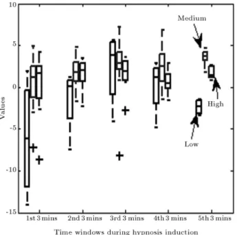
this linear combination can separate three hypnotizable groups signicantly (p-value 1.1e-011 << 0.05) during the last time window (last 3 minutes) of the hypnosis EEG. The distributions of this feature, in dierent three minute time windows during hypnosis suggestion, were represented in Figure 1 using a box plot [50]. This gure allows us to visually follow the changes of the obtained feature in three groups during hypnosis induction. It should be noted that the last 3 minutes of hypnosis EEG were considered for calculating the mentioned linear combination, but the obtained coecients (Mi) have been used for the
other time windows.
According to Figure 1, it is obvious that the distributions of the obtained feature in three groups have an overlap in dierent time windows during hypnosis induction. However, in the last time windows of the hypnosis, the distributions of the three groups are nearly separated from each other. Therefore,
Figure 1. The box plots of the distributions of the linear combination of the RF s of all brain channels in three hypnotizable groups in dierent three minute time windows during hypnosis suggestion.
we can state that the obtained feature, based on weighted regional frequency, can be used as a feature for classifying three hypnotizable groups at the end of hypnosis induction.
This claim was proved by implementing the fea-ture in a KNN-based classier. In this study, we deal with a problem with three classes: low, medium and high hypnotizable. The obtained feature values in three hypnotizable groups were entered to the classier as inputs. The desired output of the classier that was the level of each subject's hypnotizability, was determined by WSGS. The number of low hypnotizable subjects in our data was four, and we have used the LOO cross validation method for evaluating the results. Thus, we have set K = 3, because at least 3 numbers of the values of this group exist in the training data set. Also, by a trial and error technique, K = 3 had the best result. Using the LOO cross validation method, the average classication error is obtained as 3.13%. It should be mentioned that this error is the mean error of the classication error of all three groups.
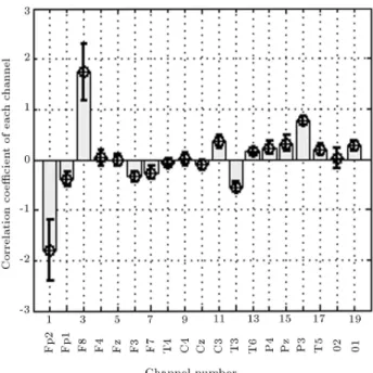
Then, it is investigated if whether or not a lower number of channels can make such a dierence between groups. This investigation was done by looking for channels that were more eective than those of others in the linear combination. The level of each channel's ecacy could be shown by its coecient (Mi) in
the obtained linear combination. The values of the obtained Mi were shown in Figure 2; these values are
validated by the LOO method. The low tolerance of the channel coecients shows that we can use the
Figure 2. The coecient values of each channel in order to make the linear combination of the RF values of all channels using LOO cross validation method.
obtained coecients for making the mentioned linear combination condently.
These coecients can show the eectiveness of each channel in the mentioned linear combination. According to these coecients, we can report that channels (FP2) and (F8) have the most eect in this linear combination. The coecient values of the channels (O2, C4, Fz, F4) and (T4), respectively, are between 0.0027 and 0.0606, so, we have considered them unimportant. Then, the linear combination was made without them, and the previous analysis was done in order to investigate the new linear combination. It was observed that the results do not have any considerable dierence from when we considered all channels in the linear combination (see the rst and second rows of Table 3).
Channels (Cz, T6, T5) and (P4) are the next channels whose coecients are less than the remaining channels. In the next stage, these channels were, respectively, removed from the linear combination, and the result of the ability of the newly produced linear combination in separating three hypnotizable groups was investigated by dierent analyses whose results were recorded in Table 3.
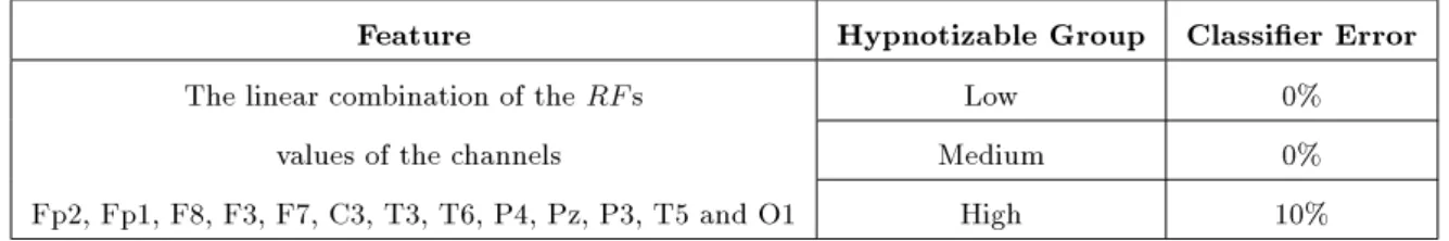
According to the recorded results in Table 3, it is seen that elimination of channel (Cz) does not have any signicant eect on the result, too. However, removing channels (T6) and (T5) makes a considerable increase in classication error. Therefore, it is resulted that the 13 channels highlighted in Table 3 are the most eective channels in the linear combination. In other words, these are the channels whose RF linear combination can determine the level of hypnotizability with the lowest error. Thus, the linear combination of these 13 channels can be replaced with the linear combination of all 19 channels. Therefore, the number of electrodes will reduce. Table 4 shows the classi-cation error of each hypnotizable group separately using the LOO cross validation method. Figure 3 shows the scatter plot of the values of the newly obtained linear combination in three hypnotizable groups.
According to the classication errors in Table 4, it is resulted that the error comes from a miss-classication in high hypnotizable groups and in ac-cordance with Figure 3, this mistake is because of the proximity of two data in high and medium hypnotizable groups (two data that are located in a circle). These data belong to two subjects whose WSGS score is 41 and 42. So, this closeness may be because of the nearness of their hypnotizability.
CONCLUSION
In this study, we introduced a feature based on weighted regional frequency, which allows
determina-Table 3. The results of investigating the ability of the linear combination of the RF s in dierent brain channels for making signicant dierence between three hypnotizable groups.
The Channels Which Contributed
in the Linear Combination p-value
1 AUC2 Classier Error3
All channels (19 channels) 1.1059e-011 0.9944 3.13% Fp1,Fp2,F8,F3,F7,Cz,C3,T3,T6,P4,Pz,P3,T5,O1 2.0230e-011 0.9944 3.13% Fp1,Fp2,F8,F3,F7,C3,T3,T6,P4,Pz,P3,T5,O1 9.6434e-011 0.9907 3.13% Fp1,Fp2,F8,F3,F7,C3,T3,P4,Pz,P3,T5,O1 3.4886e-010 0.9852 18.75% Fp1,Fp2,F8,F3,F7,C3,T3,P4,Pz,P3,O1 6.1038e-008 0.9602 37.5% Fp1,Fp2,F8,F3,F7,C3,T3,Pz,P3,O1 5.004e-006 0.9102 40.63% 1-The p-values are obtained from the ANOVA, and the null hypothesis said that there is no signicant dierence between groups.
2-The values of the AUC are obtained before performing the KNN classication.
3-The classier is based on KNN algorithm, the average error is the result of LOO validating method, and this error is the mean error of the classication error of all three groups.
Table 4. The resulting errors of the KNN based classier in each hypnotizable group using LOO cross validation. Feature Hypnotizable Group Classier Error The linear combination of the RF s Low 0%
values of the channels Medium 0% Fp2, Fp1, F8, F3, F7, C3, T3, T6, P4, Pz, P3, T5 and O1 High 10%
Figure 3. The scatter plot of the linear combination of the RF s values of the channels Fp2, Fp1, F8, F3, F7, C3, T3, T6, P4, Pz, P3, T5 and O1 in three hypnotizable groups.
tion of the level of hypnotic susceptibility of a subject by an average error of 3.13%. The separation of groups was possible only during the nal 3 minutes of hypnotic induction. Before obtaining this result, we also expected that the best separation would be done at around the end of the hypnosis induction, because from the beginning of the hypnosis induction to the end, the hypnosis depth of the subjects would increase and at about the end of the hypnosis induction the subjects would be in the nal level of hypnotizability. In other words, during the rst time windows of hypnosis induction, the hypnosis depth of the subjects are near each other and, at about the end of hypnosis induction (nal 3 minutes), the dierent hypnotizable groups stay at a dierent hypnotic depth. Thus, the separation can be done during the last time window of the hypnotic induction.
Instead of the study of Ray [26] and Behba-hani [31], who used classier algorithms for hypno-tizability level determination, the other previously EEG based studies only paid attention to nding the relation between some features and hypnotizability using statistical analyses. Therefore, we can com-pare our results only to the study results of Ray
and Behbahani. Ray found an average precision of 94% (without any cross validation) in separating the low hypnotizable groups from the high hypnotizable subjects. Behbahani reports an average precision of 93% (LOO cross validation method) in separating high hypnotizable subjects from medium and low ones. In classifying low hypnotizability, she reported high error. But, in the current study, using the obtained procedure, three hypnotizable groups can separate from each other signicantly, by an aver-age precision of 96.9% (using LOO cross validation method). Moreover, the error is not because of the low hypnotizable subject's classication, it is related to a high hypnotizable subject whose hypnotizability score is close to medium hypnotizable subjects. In other words, the RF values of high hypnotizable subjects that have medium behavior are close to medium RF values.
Calculation of the introduced feature in the cur-rent study takes about 90 seconds (using a Pentium4 with 3.2 GHz CPU). So, just after hypnosis suggestion, we can say that the subject has low, 2medium or high hypnotizability. Common clinical methods based on behavioral assessment take time to determine the level of hypnotizability and are usually boring. Also, sometimes these assessments bring the subject out from hypnosis. Therefore, in comparison with common clinical methods such as (WSGS), the introduced pro-cedure is a real time method for measuring hypnotic susceptibility. Another problem in clinical methods is that they are subjective and the subject's answers need to be trusted. But, the new method oers an objective procedure for determination of the hypno-tizability level by measuring EEG weighted regional frequencies.
REFERENCES
1. Heap, M. et al., The Highly Hypnotizable Person: The-oretical, Experimental and Clinical Issues, Routledge Pub. (2004).
2. Bowers, K.S. \Waterloo-stanford group scale of hyp-notic susceptibility, form C: Manual and response booklet", International Journal of Clinical Hypnosis, 46(3), pp. 250-268 (1998).
3. Kirsch, I. et al. \Experimental scoring for the Waterloo-Stanford group scale", International Journal of Clinical Hypnosis, 46(3), pp. 269-279 (1998). 4. Hilgard, E.R., A Stage of Hypnosis: Two Decades of
the Stanford Laboratory Hypnosis Research 1957-1979, Department of Psychology Stanford University Pub. (1979).
5. Cardea, E. and Terhune, D.B. \A note of caution on the Waterloo-Stanford group scale of hypnotic suscep-tibility: A brief communication", International Jour-nal of Clinical Hypnosis, 57(2), pp. 222-226 (2009).
6. Kaplan, H.I. and Sadock, B.J. \Comprehensive text-book of psychiatry", Lippincott Williams, Chapter 30, 3, Hypnosis (2000).
7. Temes, R., Medical Hypnosis: An Introduction and Clinical Guide, Churchill Livingstone, Pub. 1st edition (1999).
8. Stevens, L. et al. \Binaural beat induced theta EEG activity and hypnotic susceptibility: Contradictory re-sults and technical considerations", American Journal of Clinical Hypnosis, 45(4), pp. 295-309 (2003). 9. Agargun, M.Y. et al. \The Stanford hypnotic clinical
scale for adults (SHCS): Validity and reliability of the Turkish version", Sleep and Hypnosis, 9(2), pp. 102-116 (2007).
10. Gruzelier, J.H. \A working model of the neurophys-iology of hypnotic relaxation", 5th Internet Worid Congress for Biomedical Sciences, McMaster Univer-sity, Canada (1998).
11. Williams, J.D. and Gruzelier, J. \Dierentiation of hypnosis and relaxation by analysis of narrow band theta and alpha frequencies", Int J. Clin Exp. Hypn., 49(3), pp. 185-206 (2001).
12. Ray, W.J. \Understanding hypnosis and hypnotic susceptibility from a psychophysiological perspective", 5th Internet Word Congress for Biomedical Sciences, McMaster University, Canada (1998).
13. Pascalisa, V. et al. \EEG activity and heart rate during recall of emotional events in hypnosis: Relationships with hypnotizability and suggestibility", International Journal of Psychophysiology, 29, pp. 255-275 (1998). 14. Pascalis, V. et al. \Somatosensory event-related
poten-tial and autonomic activity to varying pain reduction cognitive strategies in hypnosis", Clinical Neurophysi-ology, 112, pp. 1475-1485 (2001).
15. Pascalis, V. et al. \EEG asymmetry and heart rate during experience of hypnotic analgesia in high and low hypnotizables", International Journal of Psychophysi-ology, 21, pp. 163-175 (1996).
16. Gemignani, A. et al. "Changes in autonomic and EEG patterns induced by hypnotic imagination of aversive stimuli in man", Brain Research Bulletin, 53(1), pp. 105-111 (2000).
17. Lamas, J.R. and Valle, F. \Eects of a negative visual hypnotic hallucination on ERPs and reaction times", International Journal of Psychophysiology, 29, pp. 77-82 (1998).
18. Kropotov, J.D. et al. \Somatosensory event-related potential changes to painful stimuli during hypnotic analgesia", International Journal of Psychophysiology, 27, pp. 1-8 (1997).
19. London, P. et al. \EEG alpha rhythms and suscepti-bility to hypnosis", Nature, 219, pp. 1-72 (1968). 20. Nowlis, D.P. and Rhead, J.C. \Relation of eyes-closed
resting EEG alpha activity to hypnotic susceptibility", Perceptual and Motor Skills, 27, pp. 1047-1050 (1968).
21. Morgan, A.H. et al. \EEG alpha: Lateral asymmetry related to task and hypnotizability", Psychophysiology, 11, pp. 275-282 (1974).
22. Evans, F.J. \Hypnosis and sleep: Techniques for exploring cognitive activity during sleep", Hypnosis: Research Developments and Perspectives, E. Fromm & R.E. Shor, Eds., pp. 43-83, London: Paul Elek Scientic Books (1972).
23. Dumas, R.A. \EEG alpha-hypnotizability correlations: A review", Psychophysiology, 14, pp. 431-438 (1977). 24. Perlini, A. and Spanos, N. \EEG alpha methodologies
and hypnotizability: A critical review", Psychophysi-ology, 28, pp. 511-530 (1991).
25. Gran, N.F. et al. \EEG concomitants of hypnosis and hypnotic susceptibility", Journal of Abnormal Psychology, 104(1), pp. 123-131 (1995).
26. Ray, W.J. \EEG concomitants of hypnotic susceptibil-ity", International Journal of Clinical and Experimen-tal Hypnosis, 45, pp. 301-313 (1997).
27. Abootalebi, V. et al. \Investigation of hypnosis on EEG higher order spectra", 9th Iranian Medical En-gineering Conference (2000).
28. Motie Nasrabadi, A. \Quantitative and qualitative evaluation of consciousness variation and depth of hypnosis through intelligent processing of EEG sig-nals", Bioelectric PhD Thesis, Biomedical Engineering Department, Amirkabir University of Iran (2002). 29. Horton, J.E. et al. \Increased anterior corpus callosum
size associated positively with hypnotizability and the ability to control pain", Brain, 127, pp. 1741-1747 (2004).
30. Lee, J.S. et al. \Fractal analysis of EEG in hypnosis and its relationship with hypnotizability", Interna-tional Journal of Clinical and Experimental Hypnosis, 55(1), pp. 14-31 (2007).
31. Baghdadi, G. and Motie Nasrabasi, A. \Estimation nal depth of hypnosis using extracted fractal features by EMD algorithm", 17th Iranian Conference on Elec-trical Engineering at Iran University of Science and Technology, Tehran, Iran (2009).
32. Behbahani, S., Nasrabadi, A.M. \Applications of fuzzy similarity index method in processing of hypnosis", J. Biomedical Science and Engineering, 2, pp. 359-362 (2009).
33. Escalante, T.S. et al. \Single trial P300 detection based on the empirical mode decomposition", Proceedings of the 28th IEEE EMBS Annual International Confer-ence, New York City USA, pp. 1157-1160 (2006). 34. Rutkowski, T.M. et al. \Auditory feedback for brain
computer interface management - an EEG data soni-cation approach", Springer-Verlag Berlin Heidelberg, Part III, LNAI 4253, pp. 1232-1239 (2006).
35. Sharabaty, H. et al. \Alpha and theta wave localisation using Hilbert-Huang transform: Empirical study of the accuracy", IEEE International Conference on Infor-mation and Communication Technologies, ICTTA '06, 1, pp. 1159-1164 (2006).
36. Xanthopoulos, P. et al. \Comparative analysis of time-frequency methods estimating the time-varying microstructure of sleep EEG spindles", IEEE In-ternational Special Topic Conference on Information Technology in Biomedicine (2006).
37. Cui, S. et al. \Detection of epileptic spikes with empirical mode decomposition and nonlinear energy operator", Springer-Verlag Berlin Heidelberg, LNCS 3498, pp. 445-450 (2005).
38. Huang, N.E. et al. \The empirical mode decomposition and the Hilbert spectrum for nonlinear and non-stationary time series analysis", Proc. R. Soc. Lond. A, 454, pp. 903-995 (1998).
39. Huang, W. et al. \Engineering analysis of biological variables: An example of blood pressure over 1 day", Proc. Nat. Acad. Sci. USA, 95, pp. 4816-4821 (1998). 40. Liang, H. et al. \Artifact reduction in electrogastro-gram based on the empirical model decomposition method", Medical & Biological Engineering & Com-puting, 38, pp. 35-41 (2000).
41. Wu, Z. and Huang, N.E. \A study of the characteristics of white noise using the empirical mode decomposition method", Proc. R. Soc. Lond. A, 460, pp. 1597-1611 (2004).
42. Rilling, G. and Flandrin, P. \On the inuence of sampling on the empirical mode decomposition", IEEE International Conference on Acoustics, Speech and Signal Processing, ICASSP 06, pp. 444-447 (2006). 43. Balocchi, R. et al. \Empirical mode decomposition
to approach the problem of detecting sources from a reduced number of mixtures", Proceedings of the 25th Annual International Conference of the IEEE EMBS, pp. 2443-2446 (2003).
44. Sun, L. et al. \Instantaneous frequency estimate of nonstationary phonocardiograph signals using Hilbert spectrum", Proceedings of the 2005 IEEE Engineering in Medicine and Biology, pp. 7285-7288 (2005). 45. Yang, Z. et al. \Detection of splindles in sleep EEGs
using a novel algorithm based on the Hilbert-Hung transform", Springer, Applied and Numeric Harmonic Analysis, pp. 543-559 (2006).
46. Hogg, R.V. and Ledolter, J., Engineering Statistics, MacMillan Publishing Company (1987).
47. Krzanowski, W.J., Principles of Multivariate Analysis, Oxford University Press (1988).
48. McLachlan, G.J., Discriminant Analysis and Sta-tistical Pattern Recognition, Wiley Interscience. MR1190469. ISBN 0471691151 (2004).
49. Fawcett, T. \An introduction to ROC analysis", El-sevier, Pattern Recognition Letters, 27, pp. 861-874 (2006).
50. Massart, D.L. et al. \Visual presentation of data by means of box plots", LCGC Europe, 18(4), pp. 215-218 (2005).
BIOGRAPHIES
Golnaz Baghdadi received her BS and MS degrees in Biomedical Engineering in 2006 and 2008, respectively, from Shahed University, in Tehran, Iran. Her current research interests are in the elds of Nonlinear Time Series Analysis, Blood Glucose Level Prediction and Controlling Systems, and EEG Signal Processing in Mental Task Activities.
Ali Motie Nasrabadi received a BS degree in
Elec-tronic Engineering in 1994 and his MS and PhD degrees in Biomedical Engineering in 1999 and 2004, respectively, from Amirkabir University of Technology, Tehran, Iran. Since 2005, he has been Assistant Professor in the Biomedical Engineering Department at Shahed University, in Tehran, Iran. His current research interests are in the elds of Biomedical Signal Processing, Nonlinear Time Series Analysis and Evo-lutionary Algorithms. Particular applications include: EEG Signal Processing in Mental Task Activities, Hypnosis, BCI and Epileptic Seizure Prediction.