5.6 Binary rare earth alloys

5.6 Binary rare earth alloys

The great similarity in the chemical properties of the different rare earth metals allows almost complete mutual solubility. It is therefore possible to fabricate rare earth alloys with nearly uniform electronic properties, but containing ions with disparate magnetic properties, distributed ran-domly on a single lattice. By a judicious choice of the constituents, the macroscopic magnetic properties, such as the ordering temperatures and the anisotropy parameters, may be continuously adjusted as desired. From a macroscopic viewpoint, such an alloy resembles a uniform and homogeneous crystal, with magnetic properties reflecting the character-istics and concentrations of the constituents. The spectrum of magnetic excitations also displays such average behaviour (Larsen et al. 1986), but in addition, there are effects which depend explicitly on the dispar-ity between the different sites.

We restrict ourselves to binary alloys, which are described by the Hamiltonian, H= i {c_iH1(J1i) + (1−ci)H2(J2i)} −1 2 i=j J(ij){c_iJ_1i+γ(ij)(1−c_i)J_2i} · {(c_jJ_1j+γ(ij)(1−c_j)J_2j}, (5.6.1) where c_i is a variable which is 1 if the ion on site i is of type 1, and 0 if the ith ion is of type 2. The configurational average of c_i is the atomic concentration of the type-1 ions, c_icf = c. In addition to the simplifications made earlier in the Hamiltonian, we shall assume that

γ(ij) is a constant γ, independent of i and j. This approximation is consistent with a model in which the indirect exchange is assumed to dominate the two-ion coupling, in which case

γ(ij) =γ= (g₂−1)/(g₁−1), (5.6.2) where the indices 1 and 2 refer to the two types of ions with angular momentaJ₁ andJ₂.

In order to derive the excitation spectrum of the alloy system, we first make the assumption that the surroundings of each ion are

so close to the average that individual variations can be neglected. Thus we replace the actual MF Hamiltonian of the ith ion with the configurationally-averaged MF Hamiltonian and, considering a type 1 ion (c_i= 1), obtain

H_MF(i) H_MF(i)_cf = H1(J_1i)−(J_1i−1₂J_1i)·

j

J(ij){cJ_1j+ (1−c)γJ_2j}. (5.6.3) From this equation, and the similar one for c_i = 0, we may determine the MF values of the two momentsJ₁andJ₂, and the corresponding susceptibilitiesχ₁o(ω) andχ₂o(ω). For a paramagnetic or ferromagnetic system these quantities are all site-independent, in the present approx-imation. We note that (5.6.3) is correct in the case of a paramagnet, as possible environmental variations on the individual ions are already neglected in the starting Hamiltonian. The next step is the introduction of a 2×2 matrix of susceptibility tensorsχ_rs(ij, ω), where the elements withr= 1 or 2 are defined in terms ofc_iJ_1i or (1−c_i)J_2i respectively, and s = 1 or 2 similarly specifies the other component. We may then write the RPA equation (3.5.7):

χ_rs(ij, ω) =χ_r(i, ω) δ_rsδ_ij+ j s γ_rsJ(ij)χ_ss(jj, ω) , (5.6.4a) where χ₁(i, ω) =c_iχ₁o(ω) ; χ₂(i, ω) = (1−c_i)χ₂o(ω), (5.6.4b) recalling thatc2_i =c_i (= 0 or 1), and definingJ_rs(ij) =γ_rsJ(ij), with

γ₁₁= 1 ; γ₁₂=γ₂₁=γ ; γ₂₂=γ2. (5.6.4c) In spite of the great simplification introduced through the random-phase approximation, the RPA equation for the alloy is still very complicated, because χ_r(i, ω) depends on the randomness, and it cannot be solved without making quite drastic approximations. The simplest result is obtained by neglecting completely the site-dependence of χ_r(i, ω), and consequently replacing c_i in (5.6.4b) by its average value c. This pro-cedure corresponds to the replacement of each individual angular mo-mentum J_ri by the average cJ_1i+ (1−c)J_2i, and it is known as the

virtual crystal approximation(VCA). In this approximation, (5.6.4) may be solved straightforwardly after a Fourier transformation, and defining theT-matricesaccording to

where

χ₁(ω) =cχ₁o(ω) and χ₂(ω) = (1−c)χ₂o(ω), (5.6.5b) we find that these T-matrices are given by

T_rs(q, ω) =γ_rsJ(q)D(q, ω)−1, (5.6.6a) with

D(q, ω) = 1−cχ₁o(ω) + (1−c)γ2χ₂o(ω)J(q). (5.6.6b) This result is simplified by the assumption, (5.6.2) or (5.6.4c), that J12(q) is the geometric mean of J11(q) and J22(q). In this and in

more complex cases, the introduction of the T-matrices in (5.6.5) makes it somewhat easier to handle the RPA equations. The configurationally-averaged susceptibility isχ(q, ω) =_rsχ_rs(q, ω), but this does not di-rectly determine the inelastic neutron-scattering cross-section. We must take into account the difference in the form factor{1₂gF(κ)}for the two kinds of ions, in the differential cross-section (4.2.1). At small scattering vectors,F(κ) is generally close to one and the most important variation is due to theg-factor. In this case, the inelastic scattering is proportional to the susceptibility: g2_{χ(q, ω)≡} rs g_rg_sχ_rs(q, ω) =g2₁c χ₁o(ω) +g2₂(1−c)χ₂o(ω) +χ₃(ω)J(q)D(q, ω)−1χ₃(ω), (5.6.7a) with χ₃(ω) =g₁c χ₁o(ω) +g₂(1−c)γ χ₂o(ω). (5.6.7b) If χ_r(i, ω) only depends on c_i, as assumed in (5.6.4b), the RPA equation (5.6.4a) is equivalent to that describing the phonons in a crys-tal withdiagonal disorder, in the harmonic approximation. The possible variation of the molecular field (or other external fields) from site to site, which is neglected in (5.6.3), introduces off-diagonal disorder. If such off-diagonal disorder is neglected, the main effects of the randomness, in 3-dimensional systems, are very well described in thecoherent potential approximation(CPA) (Taylor 1967; Soven 1967; Elliottet al.1974; Lage and Stinchcombe 1977; Whitelaw 1981). In the CPA, the different types of ion are treated separately, but they are assumed to interact with a common surrounding medium. This configurationally-averaged medium, i.e. theeffective medium, is established in a self-consistent fashion. The method may be described in a relatively simple manner, following the

approach of Jensen (1984). We first consider the case where χ₂o(ω) vanishes identically, corresponding to the presence of non-magnetic im-purities with a concentration 1−c. The RPA equation (5.6.4a) may then be solved formally by iteration:

χ(ij, ω) =c_iχo(ω)δ_ij+c_iχo(ω)J(ij)c_jχo(ω)

+

j

c_iχo(ω)J(ij)c_jχo(ω)J(jj)c_jχo(ω) +· · · . (5.6.8) The VCA result is obtained by assumingcn_jcf =cn, which is incorrect sincecn_jcf=c_jcf =c. Consequently, the VCA leads to errors already in the fourth term in this expansion, or in the third term ifi=j, even thoughJ(ii) is zero. In order to ameliorate these deficiencies, we first consider the series forχ(ii, ω), wherei=j. The different terms in this series may be collected in groups according to how many times theith site appears, which allows us to write

χ(ii, ω) =c_i χo(ω) +χo(ω)K(i, ω)χo(ω) +χo(ω)K(i, ω)χo(ω)K(i, ω)χo(ω) +· · · =c_i1−χo(ω)K(i, ω)−1χo(ω), (5.6.9) where K(i, ω) is the infinite sum of all the ‘interaction chains’ involv-ing the ith site only at the ends, but nowhere in between. A similar rearrangement of the terms in the general RPA series leads to

χ(ij, ω) =χ(ii, ω)δ_ij+χ(ii, ω)T(ij, ω)χ(jj, ω), (5.6.10) where T(ij, ω) is only non-zero if i =j and, by exclusion, is the sum of all the interaction chains in which the ith site appears only at the beginning, and the jth site only at the end of the chains. Introducing this expression in the RPA equation (5.6.4), we may write it

χ(ij, ω) =

c_iχo(ω) δ_ij+J(ij)χ(jj, ω) +

j

J(ij)χ(jj, ω)T(jj, ω)χ(jj, ω). From (5.6.9), we haveχo(ω)−1χ(ii, ω) =c_i{1 +K(i, ω)χ(ii, ω)}, and a comparison of this equation forχ(ij, ω) with (5.6.10), leads to the result:

δ_ij+J(ij)χ(jj, ω) +

j

J(ij)χ(jj, ω)T(jj, ω)χ(jj, ω)

leaving out the common factor c_i. Although this means that K(i, ω) and T(ij, ω) may be non-zero even when c_i is zero, this has no conse-quences in eqn (5.6.10). In order to derive the configurational average of this equation, we make the assumption that each site is surrounded by the same effective medium. Hence K(i, ω)K(ω) is considered to be independent of the site considered, and therefore we have, from (5.6.9),

χ(ii, ω) =c_iχ(ω) ; χ(ω) =1−χo(ω)K(ω)−1χo(ω). (5.6.12) With this replacement, the configurational average of eqn (5.6.11) may be derived straightforwardly, as we can take advantage of the condition that, for instance,c_jonly occurs once in the sum overj. It is important here that the common factorc_iwas cancelled, becauseT(jj, ω) involves the sitei, making the averaging ofc_iT(jj, ω) more complicated. Intro-ducing the notationT_E(ij, ω) =T(ij, ω)

cf, we get from (5.6.11) the

CPA equation δ_ij+cJ(ij)χ(ω) + j c2_J(ij)χ(ω)T E(jj, ω)χ(ω) ={1 +c K(ω)χ(ω)}{δ_ij+c T_E(ij, ω)χ(ω)} (5.6.13) for the effective medium, which may be diagonalized by a Fourier trans-formation. Introducing the effective coupling parameter

J_E(q) =J(q)−K(ω), (5.6.14) where the scalar appearing in a matrix equation is, as usual, multiplied by the unit matrix, we get

T_E(q, ω) =J_E(q)D_E(q, ω)−1 ; D_E(q, ω) = 1−c χ(ω)J_E(q) (5.6.15) and, from (5.6.10),

χ(q, ω) =c χ(ω) +c2χ(ω)T_E(q, ω)χ(ω) =D_E(q, ω)−1c χ(ω). (5.6.16) Hence the result is similar to that obtained in the VCA, except that the parameters are replaced by the effective quantities introduced by eqns (5.6.12) and (5.6.14). These effective values are determined from the ‘bare’ parameters in terms ofK(ω). It is easily seen that we retain the VCA result, i.e.K(ω) cancels out of (5.6.15), if (5.6.12) is replaced by the corresponding VCA equationχ(ω)1−c χo(ω)K(ω)−1χo(ω).

In the casec= 1, both the VCA and the CPA results coincide with the usual RPA result. K(ω) is itself determined by the effective parameters, and (5.6.13), withi=j, leads to the following self-consistent equation

K(ω) = 1

N

q

cJ(q)χ(ω)T_E(q, ω). (5.6.17a) This result may be written

K(ω) = 1 N q J(q)D_E(q, ω)−1= q J(q)χ(q, ω) q χ(q, ω), (5.6.17b) corresponding to the condition that theeffectiveT-matrix vanishes when summed over q,_qT_E(q, ω) = 0, in accordance with our starting as-sumption, (5.6.10).

In order to derive the effective medium result (5.6.13), χ(jj, ω) in (5.6.11) was replaced byc_jχ(ω), which is an approximation, as this response depends on the actual surroundings, including the sitesi and

j. The CPA incorporates the same type of mistake as in the VCA, but it is clear that the frequency of such errors is substantially reduced. The dependence ofχ(jj, ω) onc_iandc_j, corresponding to a site dependence ofK(j, ω), becomes relatively unimportant if the configuration number

Z is large, sinceior j may only be one of theZ neighbours of the site

j_.

The effective medium procedure is straightforwardly generalized to the case whereχ₂(i, ω) is non-zero (Jensen 1984). Again the CPA result may be expressed in the same way as the VCA result, (5.6.5–6), except that all the quantities are replaced by their effective CPA counterparts; J(q) becomesJ_E(q), given by (5.6.14), andχ_ro(ω) in (5.6.6) is replaced by χ_r(ω) = 1−γ_rrχ_ro(ω)K(ω) ₋₁ χ_ro(ω), (5.6.18) where the effective-medium parameterK(ω) is determined by the same self-consistent equation (5.6.17) as above. To a first approximation,

D_E(q, ω)−1 in this equation may be replaced by the simpler virtual-crystal result. Because of the poles in D(q, ω)−1, both the real and imaginary parts of K(ω) are usually non-zero, and the imaginary con-tribution then predicts a finite lifetime for the excitations, due to the static disorder. This leading-order result may serve as the starting point in an iterative calculation of K(ω), and thus of a more accurate CPA result.

It is much more complicated to include the effects of off-diagonal disorder. They have been considered in the papers referred to above, but

only in relatively simple models like the dilute Heisenberg ferromagnet with nearest-neighbour interactions. This model may be considered as the extreme example of off-diagonal disorder, and the CPA concept of an effective medium loses its meaning completely below thepercolation

concentration, where all clusters of interacting spins are of finite size, precluding any long-range order. If the molecular field is independent of the site considered, i.e. H_MF(i) =H_MF(i)_cf in (5.6.3), as happens in the paramagnetic case or ifJ₁=γJ₂, then the CPA result above should apply. However, except in a pure boson or fermion system, the ‘dynamical’ disorder due to thermal fluctuations introduces corrections to the RPA equation (5.6.4), with consequences of the same order of magnitude as K(ω) in (5.6.16), at least at elevated temperatures. In most magnetic systems, the two kinds of disorder may lead to damping effects of the same magnitude, and furthermore the use of the CPA result (5.6.16), without taking into account the dynamic renormalization of the RPA, occasionally leads to misleading results, as discussed for instance by Jensen (1984).

The excitations of binary heavy-rare-earth alloys have been studied much less extensively than their magnetic structures. However, the effect of 10% of Y, Dy, Ho, and Tm on the spin-wave spectrum of Tb has been examined, and the characteristic influence of the different solutes observed. The results of Larsen et al. (1986) for the Y and Dy alloys could be interpreted in terms of a simple average-crystal model, in which all sites are considered as equivalent, and the effect of the solute atoms is to modify the average exchange and the effective single-ion anisotropy. Thus Dy reduces the effective hexagonal anisotropy, and the spin-wave energy gap therefore decreases. On the other hand, Y dilutes the two-ion coupling, and therefore decreases T_N and the spin-wave energies, although the relative magnitude of the peak inJ(q) increases, extending the temperature range over which the helical structure is stable. The first excited state of the Ho ion in the Tb host lies in the spin-wave energy band, and the dispersion relation is consequently strongly perturbed (Mackintosh and Bjerrum Møller 1972).

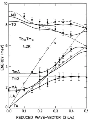
However, the most pronounced effects were observed by Larsen et al. (1988) in Tb₉₀Tm₁₀, where the Tm ions, with a spin S = 1, are relatively weakly coupled to the surrounding Tb moments, withS = 3. Furthermore, the axial anisotropy of the Tm ions is large and of opposite sign to that of Tb. As a result, well-defined quasi-localized states may be excited on the Tm sites, as shown in Fig. 5.11. These rather complex results were interpreted by means of a VCA calculation, in which the crystal-field parameters for the Tm ions were deduced from the dilute-alloy experiments of Touborg (1977), while the single-ion anisotropy and the two-ion coupling between the Tb ions were taken from the analysis

Fig. 5.11. Excitations in the c-direction of Tb₉₀Tm₁₀ at 4 K. The Tb magnon modes, the crystal-field excitations on the Tm ions, and the transverse phonons polarized parallel to the magnetization mutu-ally interfere to produce the calculated dispersion relations shown by the thick lines. The dashed lines indicate the unperturbed Tb magnons, and the short and long dashes the phonons. A and O signify acoustic and

optical respectively.

of Jensenet al.(1975) of the magnon dispersion relations. The magnon– phonon interaction, which plays an important role in determining the dispersion relations, was incorporated in the calculations by the method which will be presented in Section 7.3.1, which leads to results consis-tent with those derived in Section 5.4.2. The effective exchange between the moments on the different ions was scaled as in eqn (5.6.1–2), but

γ was given the value 0.24, instead of the 0.33 which (5.6.2) yields, in order to fix correctly the energy of the first excited state on the Tm ions. Such a departure from the simple de Gennes scaling is not partic-ularly surprising for ions with very different orbital angular momenta. In the system Pr₉₅Er₅, for example, Rainfordet al. (1988b) found that

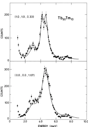
Fig. 5.12. Experimental and calculated neutron-scattering spectra in Tb90Tm10for the indicated scattering vectors, which correspond to a reduced wave-vector of 0.33 in Fig. 5.11. In the lower curve, the scattering vector is in thec-direction, while it is close to the hexagonal plane in the upper, where an unperturbed transverse phonon is observed. The ratio of the impurity intensity to the magnon peak is roughly doubled when the scattering vector moves from the c-direction to the plane, showing that the magnetic fluctuations in the impurity mode are predominantly

along thec-axis.

the Er ions modify the two-ion coupling of the host substantially. The theoretical results give a good account both of the excitation energies and of the observed neutron-scattering spectra, as illustrated in Fig. 5.12. They reveal that the difference between the interactions of the Tb and Tm ions in this alloy has a profound influence on the magnetic behaviour at the two types of site. The exchange forces the Tm moment to lie in the plane at low concentrations but, according to the calculations, the crystal fields reduce it from the saturation value of

7µ_Bto about 5.9µ_B, whereas the Tb moment is very close to saturation. Furthermore, the first excited-state on the Tm ions is at a relatively low energy, and the associated magnetic fluctuations are predominantly in thec-direction, reflecting an incipient realignment of the moments, which actually occurs at higher concentrations (Hansen and Lebech 1976). The Tb fluctuations, on the other hand, are largely confined to the plane, with the result that the neutron-scattering intensity stemming from the

c-axis fluctuations is comparable for the two types of site, even though only 10% of the ions are Tm.

The CPA theory has not yet been applied to heavy rare earth-alloys. The extra linewidth-effects due to the randomness are not expected to be very pronounced in the 10% alloys. At low temperatures, they are of the order of the contribution of the scattering against the electron-hole pair excitations of the conduction electrons, and they become decreas-ingly important compared with intrinsic effects at higher temperatures. The CPA theory has been applied to the light rare earth-alloy Pr₉₅Nd₅ (Jensen 1979a) in the paramagnetic phase, where the linewidth effects predicted by the CPA at 9 K are found to be of the same order as the intrinsic effects due to thermal disorder.