5499.pdf

(1)

CAUSAL INFERENCE IN OCCUPATIONAL

EPIDEMIOLOGY: ASBESTOS, LUNG CANCER

MORTALITY, AND THE HEALTHY WORKER SURVIVOR

EFFECT

Ashley Isaac Naimi

A dissertation submitted to the faculty of the University of North Carolina at Chapel Hill in partial fulfillment of the requirements for the degree of Doctor of Philosophy in the Department of Epidemiology.

Chapel Hill 2012

Approved by:

Stephen R. Cole

David B. Richardson

Steven B. Wing

Michael G. Hudgens

(2)

(3)

Abstract

ASHLEY ISAAC NAIMI: Causal Inference in Occupational Epidemiology: Asbestos, Lung Cancer Mortality, and the Healthy Worker Survivor Effect

(Under the direction of Stephen R. Cole)

The healthy worker survivor effect is well recognized as a potential source of bias in occupational epidemiology. Three component associations are necessary for this bias to occur: (i) prior exposure and employment status; (ii) employment status and subsequent exposure; and (iii) employment status and mortality. Together, these associations result in time-varying confounding affected by prior exposure. Previous estimates of the effect of occupational asbestos on lung cancer mortality have been obtained using methods that do not account for such confounding. Recent advances in causal inference provide key tools to examine the severity of the healthy worker survivor effect in a given cohort, and estimate an exposure-outcome relation accounting for this bias. The former relies on the use of causal diagrams developed by Pearl (2000a), allowing researchers to assess the magnitude of the component pathways in an assumed causal structure. The latter relies on the work of Robins (1989a), who introduced g-estimation of a structural nested failure time model to estimate causal effects using observational data subject to biases such as the healthy worker survivor effect.

The research for this dissertation was conducted using data from 3,072 asbestos textile factory workers hired between January 1940 and December 1965 and followed through December 2001. First, we illustrate how the component associations can be assessed using standard regression methods. For a 100 fiber-year/mL increase in cumulative asbestos, the covariate-adjusted hazard of leaving work decreased by 52% (95% confidence interval: 46, 58). The association between employment

(4)

(5)

For Adlai, my source of courage For Arielle, my little lioness For Alea, my constant support

For Mom, who sacrificed hard For Dad, who fought hard

(6)

Acknowledgments

There are too many people to thank:

Dr. Steve Cole was a fantastic mentor, and stoked in me an interest in epidemi-ology I could not have anticipated.

Drs. Lloyd Edwards and Amy Herring were central in helping me better grasp mathematical statistics.

Dr. Marshall M Joffe provided expert advice on the technical aspects of artificial censoring.

It was a pleasure to work with and learn from Alex Keil, Jess Edwards, Qianlai Luo, and Tom Stewart throughout the last four years.

Thank you Daria, Farzin, Ann, Colby, Ayla, Brad, Liz, and Naman for helping us up when we were down.

Thank you Sherlock, Ray, and Naman. It was nice to find brothers in spirit while so far away from home.

(7)

List of Tables

4.1 Uniform Job Categories & Description, reproduced from Dement (1980) 17

7.1 Potential Exposure Response Types for a Time-to-Event Outcome . . 43

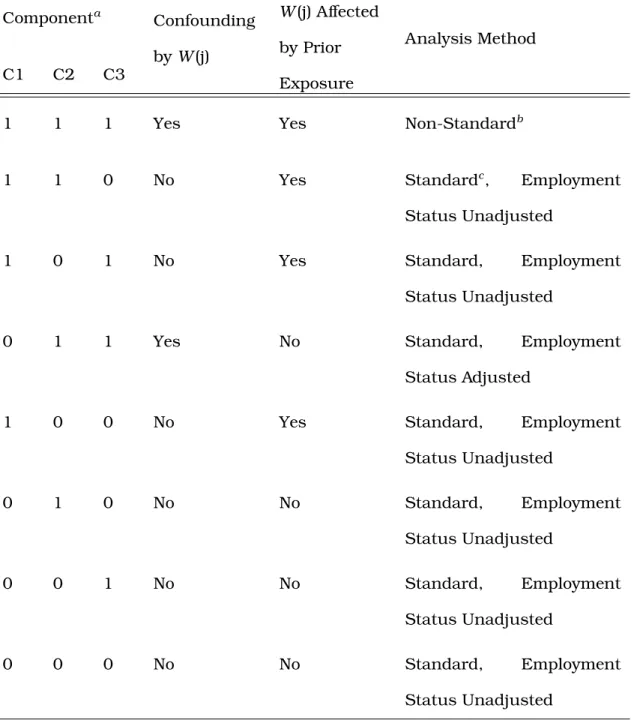
8.1 Possible scenarios and their methodological implications for the causal diagram representing the healthy worker survivor bias . . . 62

8.2 Characteristics of 2,975 individuals in the South Carolina Chrysotile Asbestos cohort . . . 66

8.3 Association between prior asbestos exposure and employment status, 2,975 individuals . . . 69

8.4 Association between employment status and subsequent asbestos ex-posure, 2,975 individuals . . . 71

8.5 Association between employment status and lung cancer mortality, 2,975 individuals . . . 74

9.1 Characteristics of 2,564 individuals in the South Carolina Chrysotile Asbestos cohort . . . 87

9.2 Survival Time Ratios (95% CIs) for the Association Between Cumulative Asbestos Exposure and Lung Cancer Mortality . . . 90

A.1 Mean estimates forψfrom 500 simulated trials each with 1,000 obser-vations. . . 108

(12)

List of Figures

2.1 Causal diagram representing the healthy worker survivor effect. . . . 10

5.1 Cumulative distribution function for lung-cancer mortality (LCM) in the South Carolina Cohort . . . 23

5.2 Log negative log of survival by log of lung cancer survival time for N =

3,072 individuals in the South Carolina Cohort . . . 24

5.3 Distribution of 120,130 person-years at risk (above y-axis break) and 198 lung cancer cases (below y-axis break) . . . 25

5.4 Mosaic plot of all 120,130 person-years on study cross-classified by race and gender . . . 26

5.5 Ambient asbestos concentrations in the facility under study from 1940 to 1977 . . . 27

6.1 Confounding triangle for the association between stork population and birth rate . . . 30

7.1 Illustration of the relation between exposure and potential outcomes defined using structural nested models . . . 54

8.1 Unadjusted Kaplan-Meier curves for the association between asbestos exposure cumulated up to the prior year and employment status . . . 68

8.2 Unadjusted dose-response trend for the association between cumula-tive exposure and employment status . . . 70

(13)

A.1 Plot of three OLS model projections and the true model from a simu-lated dataset of N =10,000 . . . 113

(14)

List of Symbols and Abbreviations

∀ Universal quantifier, read as “for all.” Used to denote that a condition must be true over the domain of the predicate.

A`

B Denotes thatA is statistically independent of B.

A `

d-sep

B Denotes thatA is topologically (or graphically) independent ofB.

¯

at For a time-varying a process, a¯t is the set of variables {a0,· · · , at}

doc-umenting the entire history of that process from its beginning at time 0 to timet.

E

{x} Expectation operator defined as R x f(x)dx taken over the support of

f(x).

f(t) The probability density function fort.

f-y/mL Fiber-years of asbestos per milliliter of air. Defined as the average num-ber of finum-bers greater than 5µm per milliliter of air to which an individual was exposed per day in a given year, times the number of years exposed.

Pa(x) The “parents” ofx, or the set of adjacent nodes on a given diagram with arrows proceeding directly into x.

Q(p) The quantile function, defined as the inverse of the cumulative distribu-tion funcdistribu-tion,F−1₍_p₎_{, with}_p_∈_[₀_,₁_]_.

Tx The potential survival time under some well defined point exposure x. Generally, superscripted variables denote potential outcomes.

X ∈Y Denotes thatX is an element in the setY.

(15)

EPA Environmental Protection Agency DAG Directed Acyclic Graph

NDI National Death Index

OSHA Occupational Safety and Health Administration UJC Uniform Job Category

(16)

Chapter 1 Introduction

1.1 Asbestos

(17)

(Camus, Siemiatycki & Meek 1998).

1.2 Asbestos and Human Health

Asbestos has long been known to have deleterious health effects, dating back even to the 1stcentury (Hunter 1969; SRI International 1978; Skinner, Ross & Fron-del 1988). The earliest known modern link between asbestos dust and death from respiratory failure was due to a report for Her Majesty’s Stationery Office in 1898 (Her Majesty’s Factory Inspectorate 1899). The authors of the report noted that the “sharp, glass-like, jagged nature of the [asbestos] particles, when allowed to rise and remain suspended in the air of a room” could explain the lung-related diseases observed in individuals working in unventilated areas (Her Majesty’s Factory Inspec-torate 1899, p172). In the early decades of the 20th century, evidence of the relation between fibrous lung diseases and asbestos exposure began to appear in the medical and scientific literature (Mehlman 1991), becoming well established by the 1930s (Castleman 2005). Around the same time, medical researchers began to suspect that asbestos had carcinogenic properties as well. A classic 1942 text on occupa-tional tumors noted reports from England, Germany, and the U.S. of “an appreciable number of cases of asbestosis [a non-cancerous fibrous lung disease] associated with carcinoma of the lung ...” (Hueper 1942, p403). By the early 1940s, European governments considered lung cancer associated with any degree of asbestosis to be an occupational disease attributable to asbestos exposure (Enterline 1991, p691). However, there was considerable debate in the American scientific community on the validity of the evidence used to classify asbestos as a carcinogen.

Prior to the 1950s, much of the evidence on the relationship between asbestos exposure and lung cancer involved case reports and clinical anecdotes, with ques-tionable and inconclusive results. It was only in the mid-1950s that more reliable

(18)

population-based epidemiologic studies began to emerge. By the early 1960s, a con-sensus was reached that asbestos did indeed have carcinogenic properties. By the latter half of the 1960s, studies began to investigate the relationship in more detail, including dose-response trends, latent periods, differential effects by asbestos type, and interactions with other known carcinogens (Castleman 2005; Michaels 2008; Weill & Hughes 1986; Enterline 1976). It was during this period of research that a more nuanced understanding of the healthy worker effect began to emerge. Realizing the scope of the problems encountered when trying to quantify the effect of an oc-cupational exposure on a health related outcome, researchers began to propose ad hoc resolutions thought to mitigate the healthy worker effect, including regression adjustment and restriction-based strategies. The research done during this period also set the stage for the governmental regulation of asbestos.

(19)

design pose substantial challenges to the consistent estimation of the causal effect an exposure on an outcome of interest: the absence of random exposure assignment, and possible complications that arise due to the presence of time-varying exposures and other covariates. The healthy worker survivor effect is a partly a consequence of these two characteristics. Unfortunately, despite their commonplace use in oc-cupational epidemiology, none of the proposed ad hoc methods could satisfactorily address either.

1.2.1 Observational versus Randomized Data

Although studies in which exposure is randomly assigned offer a protection (in expectation) against bias that is not guaranteed in an observational study, such tri-als are often infeasible in occupational epidemiology. Occupational exposures are usually suspected to be detrimental to human health, making random exposure as-signment unethical. Furthermore, compared to randomized trials, observational co-hort studies can be implemented in a more timely manner, allow for longer follow-up periods, and are usually less expensive to conduct. Because of these benefits, there has been a large body of research devoted to formalizing the conditions and assump-tions required to render exposure effect estimates obtained from observational cohort studies as comparable possible to those obtained from randomized trials (see, e.g. Hernán, Alonso, Logan, Grodstein, Michels, Willett, Manson & Robins 2008; Pren-tice, Pettinger & Anderson 2005; Benson & Hartz 2000; Concato, Shah & Horwitz 2000). Such formalization allows researchers to gain a more precise understanding of how reasonable the assumptions required in a given context are in order to in-fer causal relationships, as is done in a randomized trial, from observational data. Although this approach to causal inference using observational data finds its roots in occupational epidemiology (Robins 1986, 1987b,a), it was formalized further in

(20)

the context of HIV epidemiology (Robins 1989a, 1993; Robins, Hernán & Brumback 2000; Robins & Finkelstein 2000; Robins, Blevins, Ritter & Wulfsohn 1992; Hernán, Brumback & Robins 2001). This approach has also garnered some attention in car-diovascular epidemiology, particularly with regards to the discrepancies observed between observational studies and randomized trials on the cardiovascular effects of hormone replacement therapy (Hernán et al. 2008; Hernán, Robins & García Ro-dríguez 2005). However, a few notable exceptions aside (Robins 1986, 1987b,a; Arrighi & Hertz-Picciotto 1994; Chevrier, Picciotto & Eisen 2012), this approach has not been implemented in occupational epidemiology.

1.2.2 Time-Varying Data

(21)

OSHA, as well as the projections made by the EPA, may not be adequate. This dis-sertation is geared towards addressing certain issues involving consistent exposure effect estimation under the conditions encountered in the healthy worker survivor effect. After providing some context and describing the problem, a general framework geared towards empirically assessing the severity of the healthy worker survivor effect in a given cohort will be outlined (Part 1). For this goal, we will highlight issues in-volved in estimating associations versus causal relations, formally introduce causal diagrams, outline the logic used to assess the component associations of the healthy worker survivor effect, and carry out an empirical assessment in the cohort under study. Part 2 will be geared towards estimating the causal effect of asbestos exposure on lung cancer mortality using observational cohort data. To do this, we will define our causal estimand of interest, highlight the identifiability assumptions needed to estimate such an effect, and implement novel methods with which such assumptions can be explored and more validly justified relative to standard approaches used in occupational epidemiology.

(22)

Chapter 2 Problem Statement and Literature Review

2.1 Historical Context of the Healthy Worker Survivor

Effect

(23)

Crawford-posed particular problems for estimating the effect of an occupational exposure on a given outcome.

2.2 Methodological Approaches Aimed at Resolving the

Healthy Worker Survivor Effect

The healthy worker survivor effect has been recognized for more than 40 years (Gilbert 1982). A small number of strategies are available which attempt to overcome the bias. Two of these methods (exposure lagging and work status adjustment) have been promoted since the early 1980s, and are commonly encountered as ostensible solutions to the healthy worker survivor effect (Arrighi and Hertz-Picciotto 1993, 1994, 1996). However, these methods, though common, inadequately resolve the bias induced by the healthy worker survivor effect.

The first method used to address the healthy worker survivor effect was published in 1976 in the context of a study of the relationship between vinyl chloride monomer and angiosarcoma. In this study, Fox and Collier (1976) proposed a restriction-based method that sought to account for the selective component of the healthy worker effect. They argued that by combining their restriction-based method with an analysis stratified by work status, the selection effect would be minimized and the survivor effect significantly reduced (Fox and Collier 1976, p228). A similar method was proposed by Gilbert & Marks (1979). Using regression adjustment, these authors argued, would allow for an assessment of the effect of exposure on the outcome within subgroups of individuals with identical work status, and thus remedy the bias that results from comparing (possibly sick) individuals who left work directly to (possibly healthy) individuals who remain at work.

A year later, an alternative method was informally proposed that involved using an exposure lag (Gilbert 1982). With this method, recent exposures are ignored because

(24)

exposures nearest to the event could only have been acquired by the “survivors” that are at the root of the healthy worker survivor effect (Arrighi and Hertz-Picciotto 1996). Exposure lagging is thus a restriction-based tactic that discards information from the survivors in an attempt to put those who survive longer on an equal exposure footing with those who don’t. It attempts to overcome the bias induced by the healthy worker survivor effect by restricting the analysis to exposures that have not been acquired within a pre-specified duration prior to the event. The assumptions behind each of these methods makes it such that they are not easily substantiated as reasonable tactics. As will be explained, the issue is primarily due to the fact that individuals who leave the workplace are removed prematurely from the exposure pool due to their exposure status. Under such conditions, there is a mixing or confounding of the effect of exposure status with the effect of work status on the outcome under investigation. However, because the time at which an individual leaves work is likely influenced by their exposure history (i.e., work status is an intermediate on the path from the exposure to the outcome), the healthy worker survivor effect is not amenable to solutions involving regression adjustment, stratification, or restriction (Robins 1989b).

2.3 Limitations of Past Approaches

(25)

W

_t

X

_(t

₋

₁

₎

_X

_t

_T

U

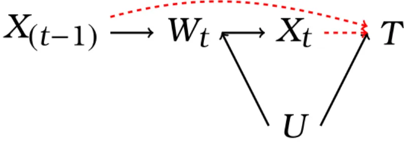
Figure 2.1: Causal diagram representing the healthy worker survivor effect.

Figure 2.1 is a causal diagram representing the healthy worker survivor effect. In this figure, we let t index time on study, X represent continuous asbestos expo-sure, W index employment status, U represent a common cause of W and T, and

T index survival time. We refer the reader to Section 6.3 for a formal description of causal diagrams and relevant terminology. Here, we simply note that the path separation criterion known as “d-separation” (Pearl 1995, 2000b, Chapter 6) dic-tates that any method that involves conditioning (e.g., regression adjustment, strat-ification) on work status Wt in order to estimate the magnitude of the dashed red

arrows in Figure 2.1 may induce collider-stratification bias by creating an artifi-cial association between prior exposure X₍t−1) and the outcome T through the path

X(t−1)→ Wt ← U →T (Hernán et al. 2004; Greenland 2003; Cole, Platt, Schisterman,

Chu, Westreich, Richardson & Poole 2010). However, not adjusting for work status results in a “d-connected” path between subsequent exposure Xt and the outcome T through the path Xt ← Wt ← U → T, and thus a confounded exposure-effect

estimate.

(26)

These issues are readily dealt with by modeling the marginal distribution of the potential outcomes using inverse probability of exposure weights to account for time varying confounders affected by prior exposure. This technique, known as the marginal structural modeling (MSM), is often an appropriate alternative to estimat-ing the effect of a time-varyestimat-ing exposure in the context of time-varyestimat-ing confoundestimat-ing (Hernán, Brumback & Robins 2000; Robins et al. 2000). However, a third complexity encountered in the healthy worker survivor effect precludes the use of MSMs as a vi-able alternative. This complication arises because workers who leave the workplace have no chance of incurring subsequent work-based exposures. This results in a violation of the positivity assumption, which is required to make inferences that are not based on interpolation or extrapolation (Hernán & Robins 2006a; Cole & Hernán 2008; Westreich & Cole 2010). Indeed, in an initial project using simulated data we have shown that the finite-sample bias of marginal structural models is similar to that of standard regression methods under conditions of time-varying confounding with positivity violations (Naimi, Cole, Westreich & Richardson 2011).

(27)

G-estimation, on the other hand, allows one to estimate such dose-response func-tions. However, implementing this method is difficult because specialized knowledge and tailored computer code is needed. Only one prior study used structural nested models to account for the healthy worker survivor effect, in which an occupational ex-posure metric that was originally measured on a continuous scale was dichotomized (Chevrier et al. 2012). One (separate) study has implemented structural nested mod-els to estimate the effect of erythropoietin dose (on a continuous scale) on mortality in patients with end stage renal disease (Joffe, Yang & Feldman 2012). No studies have used structural nested models to account for the healthy worker survivor effect in the relation between a continuous occupational exposure and mortality. The present dissertation will serve to fill this gap.

(28)

Chapter 3 Specific Aims

3.1 Rationale

Asbestos is an extremely useful, highly hazardous, and thus tightly regulated commodity in the United States. Indeed, since the mid-1950s, exposure to asbestos has been linked to a number of non-malignant and malignant disorders, the most lethal of which are lung cancer and mesothelioma. According to the Surveillance Epidemiology and End Results program, in 2004 the 5-year survival rate of mesothe-lioma (5.4%) was only about 1/3 of that of lung cancer survival (16.4%) (Surveillance Epidemiology and End Results 2004). Nevertheless, the absolute number of new lung cancer cases in the U.S. each year dwarfs the number of mesothelioma cases, and the EPA has estimated that more individuals die every year because of asbestos induced lung-cancer than mesothelioma.

(29)

tech-implement than standard methods.

3.2 Aims

In light of these issues, this dissertation seeks to address the following research questions:

1. How can researchers determine whether standard methods will suffice to es-timate the association between asbestos exposure and lung cancer mortality, or whether more complicated statistical methods such as g-estimation must be used?

2. In a dataset with an operative healthy worker survivor effect, how do the esti-mates of the effect of asbestos exposure on lung cancer mortality differ using standard methods compared to g-estimation?

3. How does g-estimation of a structural nested model perform, relative to stan-dard methods, in simulated data with a continuous exposure and time to event outcome?

3.3 Significance

This research is significant in that it will: provide researchers with an heuristic that will allow researchers to explore the severity of the healthy worker survivor ef-fect in a given cohort; provide a more accurate evidence base upon which workplace asbestos exposure can be regulated; provide a more informed understanding of the potential risks of asbestos exposure in the general population; and provide prelimi-nary evidence on the finite-sample properties of structural nested accelerated failure time models estimated using g-estimation with a continuous exposure.

(30)

Chapter 4 Study Design and Measurements

4.1 The Cohort

The South Carolina Chrysotile Asbestos study is an occupational cohort study of the relationship between workplace asbestos exposure and lung cancer mortality over a 60-year period. The cohort consisted of 3,072 individuals who worked in the plant for six months or more with at least one month of employment between 1 January 1940 and 31 December 1965 (Dement 1980). Follow-up started on 1 January 1940. Workers were followed for vital status and cause of death until loss to follow-up or administrative censoring on 31 December 2001. Date of birth, sex, and race (Caucasian versus non-Caucasian) were ascertained from company personnel records. This study was conducted on de-identified existing records and therefore deemed not human subjects research.

4.2 Mortality Ascertainment

(31)

status. Workers that were confirmed alive on 1 January 1979, and not shown to be deceased by the NDI between 1979 and 2001 were considered to be alive as of 2001. Workers lost to follow-up before 1 January 1979 were censored at the date they were last known to be alive. Prior to 1979 death certificates were obtained from the state vital records offices and the underlying cause of death was coded by a qualified nosologist. After 1979, the NDI provided underlying causes of death. All deaths were coded according to the revision of the International Classification of Diseases (ICD) in effect at the time of death. Lung cancer mortality was defined as ICD-8 and ICD-9 codes 162-163, and ICD-10 codes C33-C34.

4.3 Asbestos Exposure Assessment

Ambient asbestos concentrations were estimated for the years 1940 to 1977 (in-clusive; no individuals were employed at the facility under study after 1977) using 5,952 sampling measurements taken between 1930 and 1975 analyzed using phase contrast microscopy. As detailed in Dement, Harris, Symons & Shy (1983a), to create a job exposure matrix, the factory was divided into 9 exposure zones, each corresponding to the following physically well-defined area:

•Preparation/Waste Recovery •Draper Weaving

•Carding •Twisting

•Ring and Gang Spinning •Universal Winding

•Mule Spinning •Heavy Weaving

•Spooling (Foster Winding)

Jobs within each exposure zone were assigned to one of four uniform job cate-gories (UJC) based on the tasks associated with that job (Table 4.1).

(32)

Table 4.1: Uniform Job Categories & Description, reproduced from Dement (1980)

Category Description

A. General Area Personnel Generally in a given area, but not assigned to a specific task. Jobs include service personnel, fixers, helpers, oilers, elevator operators, doffers, clerks, supervisory personnel, etc.

B. Machine Operation Persons who normally operate textile production ma-chinery. Jobs include operators of opener machines, screens, cards, spinning frames, looms, winders, etc. C. Clean Up Persons involved in cleaning production areas. Jobs

include sweeping, cleaning of machines, etc.

D. Raw Fiber Handling Persons handling or transporting raw unspun fiber or fiber waste. Jobs include stockrollers, fly handlers, card grinders, etc.

(33)

plus an increment that was due to their association with a particular task. Using this information, Dement et al. (1983a) defined a mathematical expression for the average concentration of asbestos to which a given individual i in year on study t

was exposed. To simplify the notation, we omit the subscript i. This expression is (Dement et al. 1983a):

˜

Xtk =

X

j

˜

Cjtfjt+

X

j

∆_C˜_jtk _(4.1)

where

˜

Xtk = average number of fibers/mL air to which an individual was exposed per

day for UJCk during yeart

˜

Cjt = the baseline dust concentration, in units of chrysotile fibers longer than

5µm per mL air, for exposure zone jduring yeart

fjt = fraction of the working day spent in exposure zonejduring yeart

∆_C˜_jtk ₌ _{increment in the average concentration, in units of chrysotile fibers}

longer than 5µm per mL air, in exposure zonejdue to UJCk during yeart

The first term in Equation (4.1) provides a baseline asbestos concentration asso-ciated with being in exposure zone j. Because of the nature of the tasks associated with uniform job category A, this term corresponds to an estimate of the average exposure for job categoryA in exposure zonej. In the second term in Equation (4.1),

∆_C˜_jtk ₌ _C˜_jtk−C˜jtis the increment in the average concentration of asbestos in exposure

zonejdue to job categoryk. Note that we deviate from convention and useA˜ andY˜

to denote the average ofX and Y because in Chapters 6 and 7, we use the standard overbar notation to denote a variable’s history.

(34)

Equation (4.1) represents the mathematical model used to assign ambient as-bestos concentrations for a particular job in the factory under study. For example, suppose individual l employed in job category A in their third year on study spent half their time in exposure zone 2 and their remaining time in exposure zone 7. This individual’s estimated exposure value for their third year on study will be

˜

Xl3=C˜23×0.5+C˜73×0.5

where C˜23 is the ambient asbestos concentration in exposure zone 2 corresponding to individual i’s 3rd _{year on study (similarly for}_C_˜₇₃₎_{. As a second example, suppose}

individualm employed in job category B in their third year on study spent all their time in exposure zone 6. This individual’s estimated exposure value for their third year on study will be

˜

X63 = C˜63+ ∆C˜63B

In the right hand side of Equation 4.1, C˜jt and C˜jtk were estimated by Dement

and colleagues using a log-normal regression model with the 5,952 sampling mea-surements taken between 1930 and 1975 as the regressand (Dement et al. 1983a). This regression equation included indicators for calendar time and the time at which changes in manufacturing processes and engineering control methods occurred. The parameters for this model were estimated by Dement et al. (1983a) using ordinary least squares.

(35)

quality controlled in 1978 (Dement 1980). These records contained individual-level information onj,t,k, and fjt to use in Equation (4.1), as well as information used to

create demographic covariates. Each day during the years in which the individual was not employed was assigned a zero asbestos exposure. Each day during the years in which the individual was employed was assigned a job and calendar period specific ambient asbestos concentration in units of chrysotile fibers longer than 5µm per mL air. Following previous research (Dement et al. 1983b,a; Dement & Brown 1994; Dement, Brown & Okun 1994; Stayner, Smith, Bailer, Gilbert, Steenland, Dement, Brown & Lemen 1997; Hein et al. 2007; Richardson, Cole, Chu & Langholz 2011; Cole et al. 2012), annual exposure levels, in units of 100 fiber-years/mL, were calculated as the product of the number of days exposed in a given year and the average daily exposure values in that same year, divided by 100×365.25. We refer the reader to Section 10 for details on the interpretation of this exposure metric.

4.4 Covariate Information

Information on demographic and work history characteristics were obtained for each individual on study using detailed personnel records collected by the textile fac-tory beginning in 1930, compiled and microfilmed by the US Public Health Service in 1968, and updated, digitized, and quality controlled in 1978. These records were used to obtain information on gender, race, birth year, hire dates, termination dates, and job titles. This is information was used to create a vector of covariates to adjust for confounding of the relation between occupational asbestos exposure and lung cancer mortality. These covariates were: binary indicators for female (male referent) and non-Caucasian (Caucasian referent) individuals; a binary time-varying indica-tor of whether the individual was at work for a given year on study; and variables representing integer age and date of birth (in years).

(36)

(37)

Chapter 5 Exploratory Data Analysis

(38)

5.1 Lung Cancer Survival Time

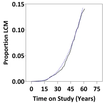
Figure 5.1: Cumulative distribution function for lung-cancer mortality (LCM) in the South Carolina Cohort.

(39)

Figure 5.2: Log negative log of survival by log of lung cancer survival time for N =

3,072 individuals in the South Carolina Cohort.

Using Figure 5.2, one can obtain an estimate of the shape parameter κ

for the Weibull distribution using the slope of the linear regression through the plotted points, which, in our case was κˆ = 2.76. Finally, Figure ?? sug-gests that some lung cancer deaths oc-curred within 10 years of being on study. This will have implications for the anal-ysis in Chapter 9, where we employ a 10-year exposure lag to examine the re-lation between cumulative asbestos ex-posure and lung cancer mortality.

Figure 5.3 demonstrates how these lung cancer cases were spread across

age, with a majority of lung cancer events occurring between ages 60 and 75, and no lung cancer deaths occurring prior to age 45. These numbers coincide roughly with figures obtained using SEER data for the years 2005-2009, which indicate that the median age at death was 72 years, and that only 1.3% of deaths due to lung cancer occurred prior to 45 years of age. In our cohort, the median age at death due to lung cancer was 67 years, with an interquartile range of (63, 74). Figure 5.3 also illustrates the distribution of person-time, with a majority of person-years falling between ages 30 and 75.

(40)

Figure 5.3: Distribution of 120,130 person-years at risk (above y-axis break) and 198 lung cancer cases (below y-axis break).

5.2 Person-Time on Study

(41)

was 46 years (interquartile range: 35, 58) and 46 years (interquartile range: 34, 57), respectively.

Figure 5.4: Mosaic plot of all 120,130 person-years on study cross-classified by race and gender.

The opposite situation occurred with ex-posure, which was similar across gen-der categories, but differential across racial categories: the median annual exposure values among female non-Caucasians and non-Caucasians was 5.9 fiber-years/mL (interquartile range: 3.0, 7.0) and 3.5 fiber-years/mL (interquar-tile range: 1.5, 4.1), respectively; the median annual concentration among male non-Caucasians and Caucasians was 5.9 fiber-years/mL (interquartile range: 2.8, 8.1) and 3.0 fiber-years/mL (interquartile range: 1.0, 4.6), respec-tively.

5.3 Annual Asbestos Exposure Values

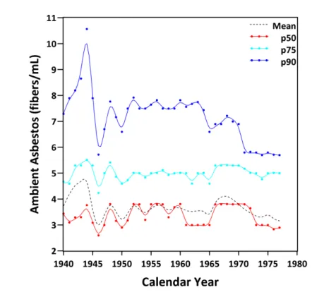
Figure 5.5 illustrates the exposure concentrations in fibers/mL in the facility under study across time. This figure represents the average, 50th percentile, 75th percentile, and 90th percentile of the individual asbestos exposures in the facility under study through time. This figure suggests that little change occurred in the exposure values over the duration of the study. Indeed, only in the highest exposure jobs did individuals in this study experience a drop in exposure values after 1944 when new exposure control mechanisms were put in place (Dement et al. 1983a).

(42)

The effects of this drop can be seen in the mean exposure values (more sensitive to outliers than the median), which are much higher pre-1944 than post-1944. Indeed, the highest exposure value over all years on study was 54.4 fibers/mL in 1942, which is an elevated but reasonable exposure value, particularly for jobs involving fiber preparation, during the period prior to 1945 when engineering controls (e.g., venting) were in place (Dement et al. 1983b). Finally, this figure illustrates that a majority of the individuals in this study experienced exposure values well within the range of permissible exposure levels issued by the Occupational Health and Safety Administration between 1971 (12 fibers/mL) and 1994 (0.1 fibers/mL).

(43)

Chapter 6 Causal Diagrams and Confounding Bias

6.1 Causation and Association in Observational

Studies

A central axiom of the present work is that epidemiologists are primarily con-cerned with estimating the causal effect of a specific exposure on a well defined health-related outcome in order to improve population health. Such effects are often estimated using observational data with tools formalized by the logic and theory of mathematical statistics. Ideally, the estimated causal effect will reflect the expected magnitude of the improvement in the health-related outcome that would be brought about by some action that would alter the level of the exposure in the target pop-ulation. In other words, the estimated effect would reflect the causal impact of the exposure on the outcome.

(44)

philosopher of science, Bertrand Russell, claimed in 1912 that “causality . . . is a relic of a bygone age, surviving . . . only because it is erroneously supposed to do no harm” (Russell 1912). Although traces of this disregard for causal inference are clearly visible in today’s statistical literature (Speed 1990; Cox 1996; Lindley & Novick 1981), the field is quickly changing.

In the early 1980s, researchers began to develop a formal theories of causal in-ference, linking them to the existing body of knowledge in mathematical statistics. These theories generally fall into two categories: the potential outcomes framework pioneered by Rubin (1974, 1978, 2005), Robins (1986, 1987b), Rosenbaum (1984, 1995), and others (Heckman & Robb 1985; Imbens & Angrist 1994; Angrist, Imbens & Rubin 1996; Imbens & Rubin 1997); and the theory of causal diagrams devel-oped by Pearl (1988, 1993, 1994, 1995), and others (Spirtes 1993; Lauritzen 1996, 2001). In the sections to follow, we will outline the main ideas behind the theory of causal diagrams, and demonstrate how they may be used to explore the component associations of the healthy worker survivor effect.

6.2 Statistical Models and Background Knowledge

(45)

area (95% confidence interval: 0.9, 4.9; p-value: 0.008). Thus, as Matthews points out, judging by statistical criteria alone, one can make the “causally nonsensical” conclusion that every 100 storks caged will serve to reduce the annual number of births by about 3 (p 38).

Storks

Area

Births

Figure 6.1: Confounding triangle for the association between stork population and birth rate.

This situation comes to a resolution once we realize that the association be-tween the stork population and birth rate is confounded by the land area of a given country. This can be conveniently demonstrated using “confounding trian-gle,” well known to epidemiologists for decades (Figure 6.1). Such figures have served as crude complements to a given

statistical analysis in an attempt to more proficiently estimate causal effects. How-ever, until the mid-1980s, the bridge between such graphical representations of confounding and an actual statistical analysis was only informal. The recent the-ory behind causal diagrams provides a convenient and logically rigorous means of formally incorporating background causal knowledge into a statistical analysis. In subsequent sections, we provide an introduction to the theory of causal diagrams, and illustrate how they may be used to explore the bias due to the healthy worker survivor effect.

6.3 Causal Diagrams, Models, and Data Generating

Mechanisms

As a scientific enterprise, epidemiology is concerned with establishing a body of knowledge on patterns that exist between exposures and health related outcomes. Bypattern, we mean a recurring set of events that repeat in a predictable manner.

(46)

For example, individuals exposed to greater amounts of occupational asbestos have shorter lung-cancer survival times. We assume that this pattern is due to certain fundamental causal processes that exist between specific components of the world. We can use graph theory to represent these fundamental causal processes in a succinct and elegant manner, and link them to the methods used in mathematical statistics.

We letGV denote the graph (or causal structure) representing the causal processes

that exist between these relevant components of the world. Following the usual graph theoretic definition, we defineGV as the ordered pair hV, Ei, where V denotes a set

of “vertices” or “nodes,” and E a set of directed “edges” or “arrows” between two nodes. The nodes inG_V represent all the relevant components of the world that take part in the causal processes linking occupational asbestos exposure to lung cancer mortality. Similarly, the edges inGV represent direct functional relationships among

the set of corresponding nodes.

For convenience we defineG ⊂ GV to be the graph containing a subset of nodes

in our data. For example, Figure 2.1 is a graphGwith nodes representing exposure

X, work status W, lung cancer survival time T, and unmeasured variables U, but without nodes representing race (denoted R), gender (denoted M), age (denoted A), and birth year (denotedB). We simply note that these latter nodes are “exogenous” in that they are not subject to any other causes relevant to our causal structure. In other words, there are no causes relevant to our interests in the relationship between occupational asbestos exposure and lung cancer mortality that influence{R, M, A, B}. Thus, for our study, we define G = h{Xt−1, Wt, Xt, U, T},{[Xt−1, Wt],[Xt−1, T],[Wt, Xt],

[Xt, T],[U, Wt],[U, T]}. Each element of E in G in the square brackets denotes an

(47)

contain additional nodes {R, M, A, B}and additional edges from each of these nodes to each of{Xt−1, Wt, Xt, U, T}. We exclude these from our graph to simplify notation,

but they are considered in all analyses.

The graph Gin Figure 2.1 is “directed” in that each edge in the graph is marked by a single arrowhead reflecting the causal order between the two nodes it connects, such as

X →W

as opposed to

X ↔W orX − W.

Furthermore, the graphGis “acyclic” in that it contains no cyclical paths starting and ending at the same node, such as

X W

Rather, in an acyclic graph, feedback loops are accommodated by subscripting nodes with their temporal ordering

Xt−δ →Wt →Xt+κ

where, for our study (due to fact that data on exposure and work status were collected annually), δ = 1, and where, for convenience, we omit the subscript κ. Our causal diagram in Figure 2.1 is a directed acyclic graph (DAG) that we denoteG. We define a “path” on DAG Gas a sequence of edges where each pair of adjacent edges in the sequence shares a node, and each such shared node can only occur once in the path. A “directed path” is a path in which the sequence edges all go in the same direction. Otherwise, the path is undirected. A “back-door” path is one in which the leading edge is directed towards the first node in the path, such as

(48)

W ←U →T.

We use kinship terminology (e.g., parents, children, descendants, ancestors) to denote the possible relationships that exist inG. For example, in Figure 2.1,Xt is a

descendant of U while U is an ancestor of Xt. Similarly, Wt is a parent of Xt while

Xt is a child of Wt. In particular, the parents of, say, W are the set of nodes from

which there is a direct arrow intoW, and are denoted Pa(W)= {Xt−1, A, R, B, M}. We restrict Pa(vj) to be only the measured parents ofvj. Finally, a node on a path with

two incoming arrows (i.e., inverted fork) is said to be a “collider” on that path. For example, on the pathXt−1 →Wt ← U → T, we callWt a collider on that path.

For a given DAG G, we say that two nodes Wt and T are unconditionally

d-separated if and only if all paths fromXt toT are blocked. A path is blocked if there

is a collider on the path, and we denote this unconditional d-separation{T ` d-sep

Wt}G

where, generally, `

is defined as “independent of.” In addition, we say that two nodesWt andT inGare conditionally d-separated if, given a set of nodesZ, all paths

between Wt and T are blocked. For conditional d-separation, a path is blocked if

there is an element in the set of nodesZ that is not a collider, or if there is a collider on the path such that neither the collider nor its descendants are in Z. We denote such conditional d-separation{T `

d-sep

Wt|Z}G.

(49)

path transmits the relevant causal information we seek to understand. The latter path transmits irrelevant information due to confounding that we seek to account for in an analysis.

Although causal diagrams (such as directed acyclic graphs) are a convenient way of encoding background knowledge about the causal processes of interest, they are of no practical use unless we make certain assumptions that link them to the statistical data we obtain for an epidemiologic study (Robins & Hernán 2009). One central assumption is known as the Causal Markov Assumption (CMA). For a given causal structure G we define a probabilistic causal model as the pair M = hG,Θi, where Θ is a set of parameters compatible with G (Pearl 2000a), and where the probability density function forMis denoted fv|Θ(v). The CMA is met when the joint

density fv|Θ(v) of the variables representing the nodes in the graph G satisfies the

Markov factorization

fv|Θ(v)= M

Y

j=1

f{vj|Pa(vj)}. (6.1)

If, for graph G, (6.1) holds, then for the statistical model M we can deduce, for instance, that

{Ta

d-sep

Wt|Z}G =⇒ {T

a

Wt|Z}M. (6.2a)

whereZ is a set of variables that block all paths fromWt toT. Note that the symbol

` d-sep

denotes a topological independence property of graphical models formally defined in Pearl (1988, 2000a), whereas the symbol `

denotes a statistical independence property defined in Dawid (1979). Pearl (1988) discusses how several authors have used Dawid’s axioms to prove graphical independence properties. Here, we simply note that under (6.1), the graphical (or topological) independence property known

(50)

as d-separation implies statistical independence for a model M consistent with G. Similarly, under (6.1),

{T

a

d-sep

Wt|Z}G =⇒ {T

a

Wt|Z}M. (6.2b)

Therefore, under certain assumptions, one can use the topological properties of a diagramGand the statistical properties of modelMto empirically assess whether the evidence in a given dataset supports the existence of certain paths on the diagram. This assessment takes on the form of a modus tollens argument:

P →Q,¬Q

∴¬P (6.2)

where

• P is the statement “the nodesWt andT on DAGGare d-connected conditional

on Pa(Wt)”, and

• Qis the statement “the variablesWt and T in modelM are statistically

depen-dent conditional on Pa(Wt)”

For this approach to work, we need only assume “compatibility,” which states that (provided our graph is correct) if two variables are d-separated, then they must be statistically independent (Rothman 2008). The compatibility assumption follows directly from the causal Markov assumption: if (6.1) holds then compatibility follows. We note that the statements in the material implication of 6.2 (i.e., the numerator

P →Q) can be switched using the transposition rule (Hurley 2011) as

¬Q→ ¬P, P

(51)

• ¬Qis the statement “the variables Wt andT in model Mare statistically

inde-pendent conditional on Pa(Wt)”, and

• ¬P is the statement “the nodesWt andT on DAGGare d-separated conditional

on Pa(Wt)”

This logic allows us to test the component associations of the healthy worker survivor effect, and obtain evidence on whether the bias due to the healthy worker survivor effect may be present in a given cohort. For this approach to work, we assume “faithfulness,” which is the logical converse of compatibility (and thus also follows directly from the causal Markov assumption). Faithfulness says that if two variables are statistically independent, they must be d-separated. This assumption is not without controversy in epidemiology (Rothman 2008, p191). The controversy stems from the fact that statistical independence between two variables may be due to either the absence of a causal relation between two variables, or the “cancellation” of the association due to some common cause (Pearl 2000b, p49). Nevertheless, due to the practical impossibility that the latter event can explain statistical independen-cies with any regularity, we follow Rothman (2008) and make the “weak faithfulness” assumption: provided our graph is correct, if two variables are statistically indepen-dent, they are most likely d-separated.

The Markov factorization 6.1 allows for a simple decomposition of the joint dis-tribution of variables represented by the nodes in G. Suppose we wish to explore whether there is empirical evidence to support the arrow in the pathX₍t−1) → Wt in G (Figure 2.1). In Chapter 8, we denote this path “component association 1.” In the Markov factorization 6.1, this would mean that our interest lies in the term of the product f(wt|Pa(wt)) = f(wt|x(t−1), a, r, b, m). We can explore this component by

specifying a statistical model for the relation such as outlined in Chapter 8, using the logic of (6.2) and (6.3).

(52)

(53)

Chapter 7 Estimating Causal Effects

7.1 Defining Causal Effects

Occupational epidemiologists are often interested in trying to understand whether the effect of an intervention on a specific occupational exposure will delay or prevent the occurrence of an undesirable health-related outcome. In the present case, as-bestos is a well-known human carcinogen (International Agency for Research on Cancer 1987). It is also, however, an extremely versatile mineral with desirable physical properties and many potential applications in commerce, industry, and re-search (Alleman and Mossman 1997). Thus, ideally, epidemiologic rere-search on the detrimental health effects of asbestos exposure would be geared towards determining optimal permissible exposure levels in an occupational setting.

(54)

this individual’s exposure history from their first year at work to their year of death as x¯t ≡ {x0,· · · , xt}, where the overbar on the x denotes the entire exposure history

(thex process) up to timet. That is,x¯t is the set of exposure values documenting the

individual’s entire exposure history since they began work until they died at timet. We refer to this set of variables denoting an exposure history as aregime. We define

T_ix¯ as the time at which individual i would have died had she been exposed to the regime defined by x¯t ≡ {x0,· · · , xt}. Similarly, we define Tx¯

0

i as the time at which this

individual would have died had she been exposed to adifferent exposure regime de-fined byx¯_t0. We define the “intervention” as the act of changing the exposure regime fromx¯t to x¯t0.

For example, let xj be the exposure value at time j just before the individual’s

cumulative history will surpass some desired cutpoint, denoted a. Then we can define the intervention “limit the cumulative amount of asbestos to which an indi-vidual is exposed to some level a” as settingx¯t ≡ {x0, x1,· · · , xt}to x¯t0 ≡ {x

0

0= x0, x10 =

x1,· · · , xj0 = xj, xj0+1 = 0,· · · , x

0

t = 0}, where

P

k≤tx 0

k ≤ a. Using the resulting variables T_ix¯ and T_ix¯0, we can assess whether capping the cumulative asbestos exposure to a

will lengthen the time to lung cancer mortality by an appreciable amount. Following Rubin (2005), for a given populationSwe define a causal effect as any comparison of the ordered sets{Tx¯

i , i ∈ S}and {T¯

x0

i , i ∈ S}. Note that this definition is not the same

as comparing the ordered sets{Tx¯

i , i ∈ S0}and{Tx¯

0

i , i ∈ S1}, S0 ,S1. The importance of this last clarification will become clear in the following paragraphs.

The variablesT_ix¯ andT_ix¯0 are potential outcomes: outcomes that would have been observed under a potential exposure regime (possibly counter to the fact) x¯t and x¯t0,

respectively. Potential outcomes such as Tx¯

i and T

¯

x0

i can be thought of as baseline

(55)

which determines which of the (possibly many) potential outcomes is observed. For example, if individual i’s observed exposure history is X¯t = x¯t, then (provided x¯t is

well-defined) the observed time to lung cancer mortality isTi = Tix¯. Consequently, all

other potential outcomes for individualiare missing: we cannot observe what would have happened to the same individual under different exposure regimes. This is a problem because our aim is to compare the ordered sets of potential outcomes (or some function thereof) for every unit i in the set of individuals defined by S under two different exposures.

This problem is known as the fundamental problem of causal inference (Holland 1986). Each potential outcome is observable, but we can never actually observe more than one potential outcome for a given individual. Thus, for a given set of individuals defined byS, we can never estimate the causal effect defined as a comparison of the ordered sets{Tx¯

i , i ∈ S}and{T¯

x0

i , i ∈ S}. Rather, we must make certain assumptions

that will give us the desired information on both T_ix¯ and T_ix¯0 for i ∈ S. Put another way, because epidemiologic data can only provide information on the ordered sets

{Tx¯

i , i ∈ S0} and {Tx¯

0

i , i ∈ S1} for S0 ⊂ S, S1 ⊂ S,S0∩ S1 = ∅, we require certain assumptions to make the information obtained from {Tx¯

i , i ∈ S0}comparable to the information obtained in{Tx¯

i , i ∈ S}(similarly forT

¯

x0

i andS1).

Finally, although defining our causal effect as any comparison of the ordered sets

{Tx¯

i , i ∈ S} and {T¯

x0

i , i ∈ S} helps acquire a general understanding of what we mean

by “causal effect,” it is too general to be of relevance to practicing epidemiologists. To make our definition more specific, we define Ti as the vector of potential outcomes {Tx¯

i , T¯ x0

i }and denote the joint density of Tgiven observed covariatesZi and observed

exposure Xi as f(t|Zi, Xi). For a given population S, this joint density defines any

causal comparison of interest. For example, one may be interested in the proportion of individuals who would not have lived past a certain age under exposure regimex¯t

(56)

andx¯_t0(doomed) compared to the proportion who would not have lived past that same age in the absence of the intervention (i.e., under exposure regime x¯t).

Epidemiol-ogists typically forego such contrasts because the required information of the joint distributionf(t|Z_i, Xi)is not identifiable with epidemiologic data (Greenland & Robins

1986; Imbens and Rubin 1997). Consequently, as will be done in the present study, it is usually sufficient to define and compare the marginal densities of Tx¯ and Tx¯0, denotedfTx¯(t|Z_i, X_i)andf_Tx¯0(t|Zi, Xi), respectively. One can then define a causal effect

as any contrast between the marginals fTx¯(t|Z_i, X_i) andf_Tx¯0(t|Zi, Xi). In particular, for

the present study, we define our causal estimand of interest as

ψ= QTx¯

0(p)

QTx¯(p)

, (7.1)

where Q_Tx¯0(·) ≡ F−1

Tx¯0(·) andQTx¯(·) ≡ F

−1

Tx¯(·)denote the quantile (or inverse cumulative

distribution) functions for argument(·), taken over the marginal distributions of Tx¯0

and Tx¯, respectively. This estimand is a measure of the relative survival time (i.e., the survival time ratio) comparingTx¯0 andTx¯. It is a summary of the horizontal dis-tance between two survival curves at any given quantile (such as, e.g., the median) denoted by p. Defining our estimand as a survival time ratio, rather than a hazard ratio (which compares attributes of the vertical space between two survival curves) is preferable because: (i) the survival time ratio has a direct physical interpretation that is more intuitive (Reid 1994); and (ii) the hazard ratio has a built-in selection bias (Hernán 2010).

7.2 Identifying Causal Effects

(57)

with epidemiologic data alone (Greenland and Robins 1986). The last three decades has seen a wide range of theoretical work devoted to formalizing conditions required to estimate causal effects. Helpful reviews include: Gutman & Rubin (2012); Pearl (2010a, 2009); Greenland & Robins (2009); Morgan & Winship (2007); Hernán and Robins (2006a); Rubin (2005); Pearl (2003); Robins (2003); Pearl (2000b,a); and Sobel (2000). Here, we give an overview of what it means for a causal effect such as defined in (7.1) to be “identifiable.” We then outline the necessary assumptions required for such identifiability to hold.

7.2.1 Identifiability

Formally, a parameter ψfor a family of distributions {f(t|ψ) :ψ∈Ψ}is said to be identifiable if distinct values ofψcorrespond to distinct probability density functions

f(t|ψ)(Casella & Berger 2002, p. 523). If a single parameter of interestψcorresponds to two or more different data generating mechanisms defined by {f(x|ψ₍_j₎) : ψ(j) ∈

Ψ} j = 1,2, . . ., we say ψ is not identifiable. We illustrate this notion using

a modified example from Greenland and Robins (1986). Consider the situation in which we wish to study the effect of the intervention defined as setting x¯t to x¯t0 (as

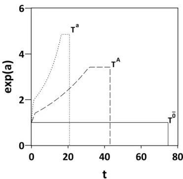
defined above) on survival time. Imagine two individuals, Person A and Person B, drawn from a target population of interest. Let T_Ag and T_Bg denote the maximum possible survival times for person A and B, respectively, under any given exposure regimeg∈[ ¯xt,x¯t0]. That is, if it has any effect at all, the intervention of changing the

regime fromg = x¯ to g = x¯0 (or vice versa) can only subtract time away fromT_Ag and

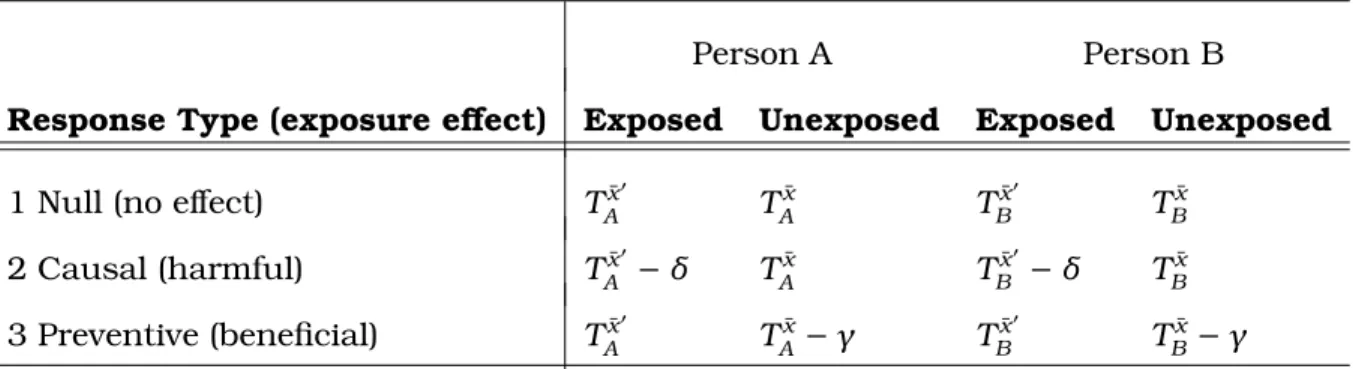
T_Bg. For each person, there are three possible response types, as displayed in Table 7.1. Letting{δ ∈_R, γ ∈_R:δ >0, γ > 0}, these response types are:

(58)

Table 7.1: Potential Exposure Response Types for a Time-to-Event Outcome

Person A Person B

Response Type (exposure effect) Exposed Unexposed Exposed Unexposed

1 Null (no effect) Tx¯0

A T ¯ x A T ¯ x0 B T ¯ x B

2 Causal (harmful) T_Ax¯0 −δ T_Ax¯ T_Bx¯0 −δ T_Bx¯

3 Preventive (beneficial) T_Ax¯0 T_Ax¯ −γ T_Bx¯0 T_Bx¯ −γ

Here, T_Ax¯0 is the potential survival time for Person A we would have observed under exposure regime x¯_t0. Without loss of generality, we refer to this regime as the “exposure,” and treat x¯t as the absence of exposure. In response type 1, the

exposure has no effect because the potential survival time for Person A we would have observed under exposure is the same that we would have observed under no exposure. In response type 2, exposure is harmful because the potential survival time for Person A we would have observed under exposure is lower (by an amount

δ > 0) than what we would have observed under no exposure. Finally, in response

type 3, exposure is beneficial because the potential survival time for Person A we would have observed under exposure is higher (by an amountγ > 0) than what we would have observed under no exposure.

Suppose we observe the exposed survival timeTx_¯0for Person A, and the unexposed

survival time Tx¯ for Person B (because exposure status is no longer potential, it

reflects group status and is indexed as a subscript). Suppose further that we contrast these observed survival times to obtain a unit-level estimate of (7.1). Our observed

Tx¯0 can only be a realization of either Tx¯ 0

A or T

¯

x0

A −δ. Similarly, our observed Tx¯ can

only be a realization of eitherT_Bx¯ orT_Bx¯−γ. Given these potential response times, our

(59)

ˆ

ψ(1) =Tx¯

0

A/T

¯

x

B: exposure has no effect

ˆ

ψ₍2) =(Tx¯

0

A −δ)/T

¯

x

B: exposure is harmful

ˆ

ψ(3) =Tx¯

0

A/(T

¯

x

B−γ): exposure is beneficial

ˆ

ψ(4) = (Tx¯

0

A − δ)/(T

¯

x

B −γ): exposure is harmful to Person A and beneficial to

Person B

A contrast of ψˆ = Tx¯0/T_x_¯0 > 1 would, unfortunately, give us no information as

to whether or not exposure to our intervention of choice was actually beneficial. A value ofψ >ˆ 1 is consistent with a number of different causal contrasts above. For example, consider three possible scenarios:

S1a. Exposure has no effect, butT_Ax¯0 > T_Bx¯: Tx¯0/T_x_¯ =ψˆ₍₁₎ >1

S2a. Tx¯0 A > T

¯

x

B and exposure decreases survival time for Person A by a factor δ > 0,

but not enough to makeTx¯0

A −δ ≤ T

¯

x

B: Tx¯0/T_x_¯ =ψˆ₍₂₎ >1

S3a. T_Ax¯0 < T_Bx¯, but the absence of exposure in Person B decreases survival by a factor

γ >0 such thatT_Ax¯0 > T_Bx¯ −γ: Tx¯0/T_x_¯ =ψˆ₍₃₎ >1

All three scenarios coincide withψ >ˆ 1. Yet, in scenario 1 exposure has no effect, in scenario 2 exposure is harmful, and in scenario 3 the absence of exposure is harmful (i.e., exposure is beneficial). Thus, a single value ofψ >ˆ 1 corresponds to a number of different possible data generating mechanisms. Hence, our causal effect is not identifiable.

Although this example is restricted to unit-level comparisons, it easily generalizes to group comparisons. For example, suppose we compared the observed survival timesTx¯0in the “exposed” groupS_A(i.e., those exposed to regimex¯0

t), and the observed

survival timesTx¯ in the “unexposed” group SB (i.e., those exposed to regimex¯t). An

5499.pdf

CAUSAL INFERENCE IN OCCUPATIONAL

EPIDEMIOLOGY: ASBESTOS, LUNG CANCER

MORTALITY, AND THE HEALTHY WORKER SURVIVOR

EFFECT

Abstract

Acknowledgments

Table of Contents

List of Tables

List of Figures

List of Symbols and Abbreviations

E

Chapter 1

Introduction

1.1

Asbestos

1.2

Asbestos and Human Health

1.2.1

Observational versus Randomized Data

1.2.2

Time-Varying Data

Chapter 2

Problem Statement and Literature Review

2.1

Historical Context of the Healthy Worker Survivor

Effect

2.2

Methodological Approaches Aimed at Resolving the

Healthy Worker Survivor Effect

2.3

Limitations of Past Approaches

W

t

X

(t

−

1

)

X

t

T

U

Chapter 3

Specific Aims

3.1

Rationale

3.2

Aims

3.3

Significance

Chapter 4

Study Design and Measurements

4.1

The Cohort

4.2

Mortality Ascertainment

4.3

Asbestos Exposure Assessment

4.4

Covariate Information

Chapter 5

Exploratory Data Analysis

5.1

Lung Cancer Survival Time

5.2

Person-Time on Study

5.3

Annual Asbestos Exposure Values

Chapter 6

Causal Diagrams and Confounding Bias

6.1

Causation and Association in Observational

Studies

6.2

Statistical Models and Background Knowledge

Storks

Area

Births

6.3

_t

_(t

₋

₁

₎

_X

_t

_T