EVALUATION OF LAVA TUBE FORMATION MECHANISMS USING THREE-DIMENSIONAL MAPPING AND VISCOSITY MODELING: LAVA BEDS
NATIONAL MONUMENT, CALIFORNIA
John DeDecker
A thesis submitted to the faculty at the University of North Carolina at Chapel Hill in partial fulfillment of the requirements for the degree of Master of Science in the
Department of Geological Sciences
Chapel Hill 2014
Approved by: Allen Glazner:
Jonathan Lees:
ABSTRACT
John DeDecker: Evaluation of lava tube formation mechanisms using three-dimensional mapping, and viscosity modeling: Lava Beds National Monument, California
(Under the direction of Allen Glazner)
I explore the relationships between lava tube morphology, estimates of lava viscosity and effusion rates, and the mechanism of lava tube formation. I calculated
effusion rates for extinct lava tubes using three-dimensional lava tube maps, and viscosity modeling utilizing data from collected samples. Lava tube lengths, effusion rate
estimates, and thermal modeling were used to evaluate the mechanisms of lava tube
formation. Lava tube lengths vs. cross-sectional radii show a positive correlation. This reflects the positive correlation observed between lava flow lengths and effusion rates in
active Hawaiian channel-fed flows. Lava tube length vs. effusion rate estimates were compared with data for Hawaiian channel-fed flows. The two data sets overlap and have parallel trends. This suggests that the lava tubes studied formed by the roofing-over of
channel-fed flows or had segments of channel-fed flow. Estimates of the lengths and mean cross-sectional radii of lava tubes can be used to evaluate whether or not extinct
lava tubes formed by the roofing-over of channel-fed flows. Length and radius estimates of extraterrestrial lava tubes could provide insight on their formation mechanism
ACKNOWLEDGEMENTS
I would like to thank the Cave Research Foundation and the University of North
Carolina Martin Fund for financing my research. I want to thank my advisor Dr. Allen
Glazner and my committee Dr. Jonathan Lees, and Dr. Kevin Stewart for their advice and
support during my research. I want to thank my field assistant Michael Gant for his
excellent work assisting me in lava tube mapping, rock sampling, and crawling through
packrat midden-filled lava tubes. I would like to thank Dr. Alan Whittington and Tony
Bollasina for their insight on viscosity modeling. I extend a special thanks to the staff of
Lava Beds National Monument for their assistance with selecting lava tubes to map, and
for their hospitality during our four-week residence at Lava Beds. Last but not least I
TABLE OF CONTENTS !
LIST OF FIGURES ... viii!
LIST OF TABLES ... xi!
1. Introduction ... 1!
2. Regional Setting ... 3!
2.1 Lava Beds National Monument ... 3!
2.1.1 The basalt of Mammoth Crater (MC basalt) ... 5!
2.1.2 Comparison with the basalt of Giant Crater ... 6!
2.2 Lava Tube Systems in the MC Basalt ... 7!
2.2.1 Headquarters Lava Tube System ... 10!
2.2.2 Bearpaw-Skull Lava Tube System ... 11!
3. Methods ... 12!
3.1 Lava Tube Mapping ... 12!
3.2 Sample collection ... 15!
3.3 X-Ray Fluorescence ... 16!
3.4 Scanning Electron Microscope ... 16!
3.5 Petrography ... 17!
3.6 Viscosity Modeling ... 18!
3.8 Thermal modeling ... 18!
3.8.1 Thermal budget for master tubes ... 19!
3.8.2 Thermal budgets for near-surface tubes ... 20!
4. Results ... 21!
4.1 Lava Tube Morphology ... 21!
4.2 Rock Compositions ... 25!
4.3 Petrography ... 28!
4.4 Viscosity modeling ... 30!
4.5 Thermal modeling ... 34!
5. Discussion ... 39!
5.1 Compositional Zonation of MC Basalt ... 39!
5.2 Lava viscosity ... 40!
5.3 Lava tube morphology ... 41!
5.4 Thermal Modeling ... 47!
5.5 Significance for evaluating extra-terrestrial lava tube caves ... 48!
6. Conclusions ... 49!
APPENDIX 1: MAP DATA FOR HERCULES LEG - JUNIPER CAVE ... 50!
APPENDIX 2: MAP DATA FOR SUNSHINE CAVE ... 67!
APPENDIX 3: MAP DATA FOR VALENTINE CAVE ... 71!
APPENDIX 4: MAP DATA FOR C-TUBE, PISGAH CRATER ... 78!
APPENDIX 5: COMPOSITIONAL ANALYSIS OF NON-MC BASALT SAMPLES ... 82!
APPENDIX 7: PARAMETERS USED IN THERMAL BUDGET
CALCULATIONS ... 84
LIST OF FIGURES
Figure 1 - The region surrounding Lava Beds National Monument. ... 4
Figure 2 -A view from Captain Jack's Stronghold looking
southwest towards Medicine Lake shield volcano. ... 5
Figure 3 - (a) SRTM 10m digital shaded relief map of the region near Lava Beds National Monument. (b) A geologic map of the same area as (a), from
Donnelly-Nolan and Champion (1987) and
Donnelly-Nolan (2010).. ... 9
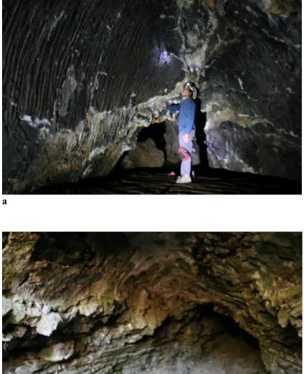
Figure 4 - a) The well-preserved melt lining in Hercules Leg-Juniper Cave. b) A section of the Bearpaw
Butte tube where the melt lining has been removed. ... 11
Figure 5 - The rendering of maps consists of: (a) plotting the line between stations, (b) translating rotated cross-section points to their corresponding station, and (c) plotting cross-sectional polygons and lines between corresponding cross-sectional points at
successive stations.. ... 14
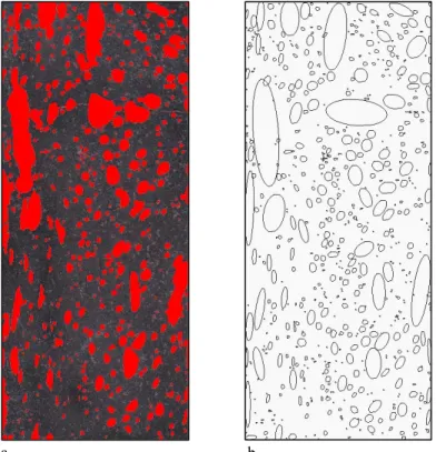
Figure 6 - The method for determination of vesicle dimensions, (a) scanned and color thresholded image of sample HL-2 with dyed gypsum-filled vesicles in red, and (b) drawing of best fit ellipses determined by ImageJ that were used to calculate
mean major and minor axes of vesicles. ... 17
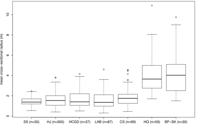
Figure 7 - Boxplots of the mean cross-sectional radii for survey stations in lava tubes mapped by the author
and Waters et al. 1990 in the MC basalt.. ... 22
Monument, Mount St. Helens, and Pisgah Crater. ... 23
Figure 9 - Aspect ratios for lava tube caves in the MC basalt, and for tubes within other flows at Lava Beds National
Monument, Mount St. Helens, and Pisgah Crater. ... 24!
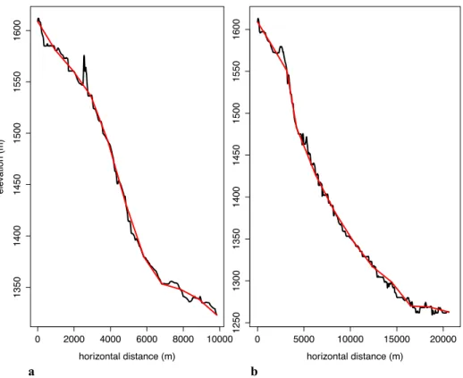
Figure 10 - Elevation profiles for the Headquarters (a) and
Bearpaw-Skull (b) master tubes.. ... 24
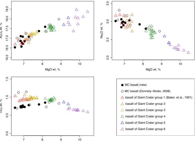
Figure 11 - Magnesium variation plots of MC basalt and
basalt of Giant Crater samples. ... 28
Figure 12 - Reversely zoned plagioclase xenocrysts in sample J-LS. ... 28
Figure 13 - Backscattered electron image of a reversely zoned plagioclase xenocryst in sample J-N6 from
Hercules Leg-Juniper Cave. ... 30
Figure 14 - (a) Calculated melt and effective viscosities for anhydrous MC basalt samples, and (b) calculated melt and effective viscosities for MC basalt samples
containing 1 wt.% H2O, plotted as a function of SiO2 wt.%. ... 33
Figure 15 - Measured lava tube length vs. estimated tube-full effusion rates compared with channel and tube-fed flow observations (circles and asterisks) from Fig. 1 of
Pinkerton and Wilson (1994).. ... 45
Figure 16 - A skylight in Sunshine Cave showing the tube lining and re-melt features on the interior of the
tube, and layering between the tube ceiling and the surface. ... 46
Figure A1 - Map view of Hercules Leg-Juniper Cave ... 64
Figure A3 - Oblique view of Hercules Leg-Juniper cave looking southwest ... 66
Figure A4 - Map view of Sunshine Cave ... 70!
LIST OF TABLES
Table 1 - Summary statistics for lava tube map data ... 21
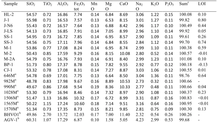
Table 2 - Whole rock major element analysis of Basalt of Mammoth Crater ... 26
Table 3 - Modal mineralogy, volume fraction of crystals, vesicles, and groundmass ... 29
Table 4 - Size comparison between plagioclase phenocrysts and vesicles ... 29
Table 5 - Calculated melt and effective viscosities of MC basalt samples ... 31
Table 6 - Calculated cooling for Headquarters and Bearpaw-Skull master tubes ... 35
Table 7 - Calculated cooling for near-surface tubes ... 38!
Table A1 - Line-plot data for Hercules Leg-Juniper Cave ... 50!
Table A2 - Hercules Leg – Juniper Cave cross-section data ... 55!
Table A3 - Line-plot data for Sunshine Cave ... 67!
Table A4 - Sunshine Cave cross-section data ... 68!
Table A5 - Line-plot data for Valentine Cave ... 71
Table A6 - Valentine Cave cross-section data ... 73
Table A7 - Line plot data for C-tube, Pisgah Crater ... 78
Table A9 - Whole rock compositions for samples from Ape Cave, Valentine Cave, Caldwell Ice Cave,
and Pisgah Crater ... 82!
Table A10 - Modal mineralogy, volume fraction of crystals, vesicles, and groundmass for samples from Ape Cave, Valentine Cave, Caldwell Ice Cave,
and Pisgah Crater used in volumetric flow rate calculations ... 83!
1. Introduction
Lava tubes are thermally insulated subsurface conduits capable of transporting lava several kilometers from the source vent (Swanson, 1973). They form by the roofing-over of channel-fed flows (Dragoni et al., 1995), or the formation of shear surfaces within the interior of a pahoehoe flow (Greeley and Hyde, 1971). Lava tube caves form if the tube has sufficient topographic gradient and a down-tube exit allowing lava to drain from the tube. Lava tube cave skylights and collapse trenches are found in basalt and basaltic andesite flows on Earth, Mars, and the Moon (Greeley and Hyde, 1971; Greeley and Guest, 1977; Cushing, 2012). NASA is considering using lava tube caves as natural radiation shelters for future human missions to Mars (Wynne et al., 2008).
The majority of work on terrestrial lava tubes has focused on observations and modeling of actively forming lava tubes and channels at Kilauea on the island of Hawaii. Pinkerton and Wilson (1994) established that Hawaiian tube-fed lava flows and channel-fed lava flows exhibit different length-effusion rate relationships. The final length of a channel-fed flow is positively correlated with lava effusion rate, whereas exclusively tube-fed flows show no correlation between length and effusion rate (Pinkerton and Wilson, 1994; Harris and Rowland, 2009). Channel-fed flows cool primarily by thermal radiation and convection of air from the flow surface. As lava cools the viscosity
relationship because the thermal insulation provided by lava tubes substantially reduces the rate of cooling with distance. Calculated cooling-limited lengths for terrestrial lava tubes can exceed 100 km (Keszthelyi, 1995). Terrestrial tube-fed flows rarely exceed tens of kilometers; consequently most tube-fed flows are considered volume-limited in length. Volume-limited tube-fed flows reach their terminal lengths when the lava supply feeding them is exhausted (Harris and Rowland, 2009).
Relatively little work has focused on inactive lava tube caves, besides two-dimensional mapping, general descriptions, and interpretation of small-scale flow features (Greeley and Hyde, 1971; Waters et al., 1990). The primary objectives of this study are to integrate three-dimensional mapping of lava tube caves with numerical models relating tube shape, estimated lava viscosity, lava effusion rate, and the thermal behavior of lava tubes in an effort to evaluate lava tube formation mechanisms. If there is a relationship between lava tube cave length, slope, cross-sectional radius, and the
mechanism of lava tube formation, then it may be possible to use remote sensing to evaluate lava tube formation mechanisms on the Moon and Mars.
I present the results of three-dimensional mapping, and compositional and
petrographic analysis of collected samples. Using these primary data I modeled effective viscosities of the samples between 1080-1160 °C and 0-1 wt.% H2O, estimated effusion
2. Regional Setting
2.1 Lava Beds National Monument
Lava Beds National Monument, California is on the north flank of Medicine Lake volcano, a shield volcano 50 km east of Mt. Shasta at the junction of the Cascade
volcanic arc and the Basin and Range province in northern California (Figs. 1,2). Eruptions at Medicine Lake volcano began ca. 500 ka; erupted products vary
compositionally from primitive basalt to rhyolite (Donnelly-Nolan, 2010). I chose Lava Beds National Monument as the field area for this study because of the over 400 lava tube caves present, the well-preserved nature of many of the caves, and the compositional variation observed within the dominantly tube-fed basalt of Mammoth Crater (Waters et al., 1990; Donnelly-Nolan et al., 1991; Larson, 1991), called MC basalt herein.
Figure 1 The region surrounding Lava Beds National Monument.
Medicine Lake Volcano Lava Beds National Monument Casacade
Volcanic Arc
Cascade Volcanic Arc
Basin and Range Province
Sources: Esri, HERE, DeLorme, USGS, Intermap, increment P Corp., NRCAN, Esri Japan, METI, Esri China (Hong Kong), Esri (Thailand), TomTom, MapmyIndia, © OpenStreetMap contributors, and the GIS User Community, Sources: Esri, DeLorme, USGS, NPS, Sources: Esri, USGS, NOAA
120°0'0"W 120°0'0"W
120°30'0"W 120°30'0"W
121°0'0"W 121°0'0"W
121°30'0"W 121°30'0"W
122°0'0"W 122°0'0"W
122°30'0"W 122°30'0"W
123°0'0"W 123°0'0"W
43°0'0"N 43°0'0"N
42°30'0"N 42°30'0"N
42°0'0"N 42°0'0"N
41°30'0"N 41°30'0"N
41°0'0"N 41°0'0"N
40°30'0"N 40°30'0"N
0 20 40 80 120
Kilometers
Mt. Shasta
$
Figure 2 A view from Captain Jack's Stronghold looking southwest towards Medicine Lake shield volcano and it's parasitic cinder cones. Mount Shasta is visible to the extreme right.
2.1.1 The basalt of Mammoth Crater (MC basalt)
The MC basalt is compositionally zoned from basaltic andesite to high-alumina basalt (Donnelly-Nolan et al., 1991). The duration of the eruption of the MC basalt is estimated to be ~10-30 years based on paleomagnetic data (Donnelly-Nolan and Champion, 1987; Waters et al., 1990). The volume of the Mammoth Crater eruption is estimated at ~4.2 km3 and the flow covers an area of ~250 km2.
2.1.2 Comparison with the basalt of Giant Crater
The basalt of Giant Crater was emplaced in 6 eruptive phases that progressed from basaltic andesite to high-alumina basalt (Baker et al., 1991; Donnelly-Nolan et al., 1991). The total erupted volume of the basalt of Giant Crater is estimated to be ~4.4 km3.
Baker et al. (1991) proposed a magma model for the basalt of Giant Crater involving repeated intrusions of high-alumina basalt into granitic crust beneath Medicine Lake Volcano. The initial intrusion of basalt differentiated to a ferrobasalt by the
formation of a Mg-rich cumulate, and partially melted and assimilated granitic country rock. The presence of resorbed, reversely zoned plagioclase and quartz xenocrysts supports the conclusion that crustal assimilation played a role in producing this compositional variation (Baker et al., 1991). Subsequent basalt intrusions initiated convective mixing and generated a density-stratified basaltic magma body capped by basaltic andesite. The basaltic andesite erupted first and was followed by progressively more mafic basalts as the proportion of crustal assimilant to high-alumina basalt decreased as lower levels in the magma body were tapped. The compositional gap
between 49.7 and 50.4 wt. % SiO2 coincides with a pause in eruptive activity indicated by
paleomagnetic evidence (Champion and Donnelly-Nolan, 1994).
2.2 Lava Tube Systems in the MC Basalt
The MC basalt was predominantly transported by five master tube systems. Master tubes are typically the most mature lava tubes in a flow, have relatively large cross-sectional radii and aspect ratios, and transport the largest volume of lava in a tube-fed flow system. Distributary tubes are typically near the surface, have relatively small cross-sectional radii and aspect ratios, and do not transport as much lava as master tubes.
a
121°28'0"W 121°28'0"W
121°30'0"W 121°30'0"W
121°32'0"W 121°32'0"W
121°34'0"W 41°48'0"N
41°48'0"N
41°46'0"N
41°46'0"N
41°44'0"N
41°44'0"N
41°42'0"N
41°42'0"N
0 2Kilometers
Former lava lake
$
Bearpaw-Skull Master Tube
Headquarters Master Tube
Near-surface tubes Bearpaw-Skull
Master Tube Bearpaw Butte
tube
Bertha's Cupboard and Valentine Caves
Caldwell Ice Caves
Elevation (m)
Image
Value
High : 2000
Low : 1200
Craig Cave Captain Jack's Stronghold
b
Figure 3 (a) SRTM 10m digital shaded relief map of the region near Lava Beds National Monument. Positions for the former lava lake and the Headquarters distributary system are from Waters (1990) and Donnelly-Nolan and Champion (1987). A segment of the Headquarters system is inferred to lie under the younger basaltic andesite of Valentine Cave and resurface at an entrance to Craig Cave immediately east of the basaltic andesite of Valentine Cave (Waters, 1990). (b) A geologic map of the same area as (a), from Donnelly-Nolan and Champion (1987) and Donnelly-Nolan (2010). Flow units and tube systems that were studied are noted with bold black labels.
MC basalt 121°28'0"W 121°28'0"W 121°30'0"W 121°30'0"W 121°32'0"W 121°32'0"W 121°34'0"W 41°48'0"N 41°48'0"N 41°46'0"N 41°46'0"N 41°44'0"N 41°44'0"N 41°42'0"N 41°42'0"N
0 2 Kilometers
Former lava lake
$
MC basalt
basaltic andesite of Valentine Cave Bearpaw-Skull Master Tube Headquarters Master Tube Near-surface tubes Bearpaw-Skull Master Tube Bearpaw Butte tube
Bertha's Cupboard and Valentine Caves
Caldwell Ice Caves
Craig Cave Captain Jack's Stronghold
2.2.1 Headquarters Lava Tube System
The Headquarters system consists of a master tube that begins in a former lava lake near the vent at Mammoth Crater and trends downslope to the northeast at least as far as Craig Cave, ~11 km down-tube from the vent (Fig. 3). Some segments of the master tube have collapsed forming collapse trenches between intact tube segments. Near the Natural Bridge segment of the master tube the lava tube morphology changes as several overflow lobes hosting near-surface distributary lava tubes emerge from and surround the master tube and continue downslope ~2 km (Waters et al., 1990; Larson and Larson, 1990).
Caves comprising the distributary segment of the Headquarters system are: Hercules Leg-Juniper, Sunshine, Catacombs, Labyrinth, and Hopkins Chocolate-Golden Dome. The distributary tubes occur within lava overflow lobes that formed when
a
b
Figure 4 a) The well-preservedmelt lining in Hercules Leg-Juniper Cave obscuring lava stratigraphy. b) A section of the Bearpaw Butte tube where the melt lining has been removed exposing a layered structure in the walls.
2.2.2 Bearpaw-Skull Lava Tube System
The Bearpaw-Skull lava tube systemconsists of a chain of master tube segments and collapse trenches ~20 km in length within the MC basalt. It begins at the intersection with the Headquarters master tube in the former lava lake and terminates in the northern part of the monument south of Captain Jack’s Stronghold (Fig. 3).
3. Methods
3.1 Lava Tube Mapping
Hercules-Leg Juniper and Sunshine caves were mapped in three dimensions using methods developed by Ruby et al. (2011) and herein. We set up survey stations by
placing flagging at locations where the tube noticeably bent, changed cross-sectional shape, changed slope, bifurcated, or intersected another survey line. Distance (D),
azimuth (A), and inclination (I) from one station to the next define a spherical coordinate system. These data provide a means of rendering a line plot of a lava tube in three
dimensions.
Measuring front- and back-azimuths between survey stations minimized compass error due to magnetic minerals. If these azimuths differed by <5 degrees then the mean value was taken as the azimuth. In the event of discrepancies between the front- and back-azimuth >5 degrees, we measured the angle between the vector from the previous station and the vector to the next station using the accelerometer-based 3D Protractor app on an iPad. We took all azimuth measurements from each survey station to an illuminated station of known height located at the next survey station.
azimuth to the next station. Each cross-section consists of 12 (r, θ) measurements taken in 30° increments of θ.
Cross-sectional data were converted from polar to Cartesian coordinates. Each set of cross-sectional plane points was rotated from an initial azimuth of 0° to the measured azimuth (A) using a three-dimensional rotation matrix with an angle of rotation about the y-axis of 2π – A. Line plots were constructed using D, A, and I to!define a spherical coordinate for the position vector to the next station. Each rotated cross-section was translated to its corresponding position vector, generating a point cloud of the lava tubes mapped (Fig. 5).
! !!
!
! !!!!!!!a! ! ! ! ! !b!
Z
X Y
Z
!
! ! c!
Figure 5 The rendering of maps consists of: (a) plotting the line between stations, (b) translating rotated cross-section points to their corresponding station, and (c) plotting cross-sectional polygonsand lines between corresponding cross-sectional points at successive stations. The example shown here is the middle segment of the Hercules Leg-Juniper cave. The axes scale is 50 m along each axis.
!
I determined the length of the main- and side-passages by summing the distances between each station along the line plot. The overall slope of the tubes mapped was determined in three independent ways to check for accumulation of error due to the large number of stations in the caves mapped. The first method calculated slope using the total elevation drop (y-axis) and dividing it by the total length of the main passage. The second method utilized a TruPulse 360 laser rangefinder to measure D, A, and I on the surface between survey stations located on skylight rims. The final method used 10 m resolution SRTM digital elevation maps with overlain orthoimagery to construct an elevation profile in ArcMap 10.1.
I used this last method to determine the lengths and slopes of the master tubes, as well as the slopes for lava tube caves not mapped in this study but with previously existing 2-D cave map data with width and height measurements noted (Waters et al., 1990). All lengths for lava tubes include the total length of the main cave passage
Y
X
mapped as well as the distances between collapse pits and trenches near to and along-trend with the main-passage observed in orthoimagery.
Cross-sectional data for the Headquarters and Bearpaw-Skull master tubes consist of height and width measurements taken with a laser rangefinder. I used height and width measurements from mapping done by Waters et al. (1990) to supplement cross-sectional radius data for both master tubes, as well as Catacombs, Labyrinth, and Hopkins
Chocolate–Golden Dome Caves. Aspect ratios were calculated for each cross-section by dividing the height by the width, and then the arithmetic mean of all aspect ratios in each tube was calculated.
3.2 Sample collection
I collected samples from Hercules Leg-Juniper and Sunshine caves, members of the Headquarters distributary system, at several locations along the Bearpaw-Skull master tube, and from Captain Jack’s Stronghold (Fig. 3). Samples were collected in
inconspicuous locations without damaging a cave’s appearance or structural integrity. Samples collected from Hercules Leg-Juniper and Sunshine caves are: loosened ceiling rocks at skylights (HL-2, SS-3), a piece of ceiling-collapse slab found below its pre-collapse position (J-1), a collapsed ceiling block with attached lavacicle (J-N6), a piece of aa (J-LS) from an unusually steep-sloped lava spring, and a loosened piece of floor pahoehoe (SS-1).
blocking the entrance to a cave in the wilderness area of Lava Beds National Monument (locations for samples collected in the wilderness area are undisclosed as per monument regulations). A sample (CJ-1) was collected from a tumulus south of Captain Jack’s Stronghold northwest of the terminus of the Bearpaw-Skull system.
3.3 X-Ray Fluorescence
Samples were crushed in a jaw crusher and pulverized in a pre-contaminated alumina-ceramic shatter box. Loss on ignition was performed on all samples in a muffle furnace at 950°C for 1 hr. Fused glass disks were prepared with a Katanax K-1 fluxer using 0.9000 ±0.0005 g of sample and 8.1000±0.0005 g of Li metaborate-tetraborate flux. Major-element XRF analyses were performed on a Rigaku Supermini XRF spectrometer, using calibration standards AGV-1, BHVO-1, MAG-1, QLO-1, GSP-1, DNC-1, and BIR-1. All results were normalized to 100 wt.% volatile-free.
Eleven new whole-rock analyses for the basalt of Mammoth Crater are supplemented with previous analyses reported by Donnelly-Nolan (2008). Iron was measured as Fe2O3, converted to FeO total by multiplying Fe2O3 by 0.8998, and
compositions were normalized to 100 wt.% before input into the viscosity calculation.
3.4 Scanning Electron Microscope
Sample J-N6, a lavacicle roof-collapse block from Juniper Cave, was examined using backscattered electron imaging in a Tescan Vega 5130 scanning electron
3.5 Petrography
Standard 27x46 mm thin sections were made of each sample analyzed by XRF except SS-1 and J-N6. The volume fraction of phenocrysts, vesicles, and groundmass was determined by point counting (n=1,000), using a mechanical stage at a magnification of 10x. The sizes of phenocrysts were measured using calibrated digital photomicrographs.
I determined vesicle sizes by cutting samples into billets, polishing a side, filling the vesicles with a gypsum-water paste dyed blue, allowing the gypsum filler to dry, sanding the surface of the billets clean with 1000-grit sandpaper, and scanning the billets with a digital scanner (Fig. 6). ImageJ (http://rsb.info.nih.gov/ij/) was used to scale and analyze dimensions of the best-fit ellipses for filled vesicles > 1 mm2 in area. !
a b
3.6 Viscosity Modeling
I calculated melt viscosities using the model developed by Giordano et al. (2008). Giordano’s model estimates silicate-melt viscosity using a calibration against empirical viscometry experiments on a wide range of magma compositions (see
http://www.eos.ubc.ca/~krussell/VISCOSITY/grdViscosity.html for details about this model). The effect of crystals and vesicles on lava viscosity was accounted for using a three-phase (melt, crystals, and vesicles) effective viscosity model developed by Harris and Allen (2008).
3.7 Effusion rates
The Hagen-Poiseuille equation was used to estimate tube-confined gravity-driven effusion rates (Sakimoto et al., 1997) using measured mean radius and slope data,
estimated effective viscosity values, and densities of 1560 and 2600 kg/m3 for 0.4 vesicle fraction and vesicle free basaltic lavas respectively (Keszthelyi, 1995; Kerr, 2001). The Hagen-Poiseuille equation is:
! =!!!
8! !"sin!
where ! is the effusion rate, ! is the cross-sectional radius of the tube, ! is the effective viscosity of the lava, ! is the density of the lava, ! is gravitational acceleration, and ! is the slope of the lava tube.
3.8 Thermal modeling
was used to estimate thermal erosion rates. I used an initial temperature of 1150 °C for all thermal models. This value agrees with observations of Hawaiian tube-fed flows
(Pinkerton et al., 2002). Constant parameters used in thermal modeling are given in Appendix A7.
3.8.1 Thermal budget for master tubes
I calculated thermal budgets for both master tubes by dividing the elevation profile data for each tube into ten segments consisting of approximately the same number of data points per segment. I used the mean radius of the lava tube modeled for all
segments but divided the second segment of the Bearpaw-Skull tube into two segments consisting of the same number of data points. This was done to better approximate the change in slope occurring ~5000 m from the beginning of the tube. The elevation profiles for the Headquarters and Bearpaw-Skull master tubes and the segments used in the thermal budget models are illustrated in Figure 8. The number of skylights in the master tubes is unknown due to significant collapse of several sections of both master tubes, so I assumed two skylights per kilometer for !!"#calculations. This assumption is based on the approximate number of skylights per kilometer for intact segments of the Bearpaw-Skull tube as mapped by Waters et al. (1990).
Calculated effective viscosities at 1150 °C of sample CJ-1 (anhydrous, 0.1 and 1.0 wt.% H2O) were used as the initial viscosity input into thermal budget models for both
3.8.2 Thermal budgets for near-surface tubes
The thermal budgets for the near-surface tubes surrounding the Headquarters master tube were modeled using a single segment and the mean radius for each tube. For simplicity only the main passage in each tube was considered in thermal budget
calculations. Skylights noted during mapping or by previous workers were used for
!!"#calculations.
The calculated effective viscosities at 1150 °C of sample HL-2 (anhydrous and 1.0 wt.% H2O) were used as input into thermal budget calculations for Hercules Leg–
Juniper Cave (where the sample was collected), and for Hopkins Chocolate-Golden Dome Cave, Labyrinth Cave, and Catacombs Cave where samples were not collected. The calculated effective viscosities at 1150 °C of sample SS-3 (anhydrous and 1.0 wt.% H2O), were used as input into thermal budget calculations for Sunshine Cave. I used
4. Results
4.1 Lava Tube Morphology
The arithmetic mean radii were determined for each cross-section in a cave. Boxplots showing the distribution of mean cross-sectional radii for each tube are given in Figure 7. The lava tubes studied group into two distinct populations based on their
median sectional radius. Summary statistics for the population of all mean cross-sectional radii in a cave (excluding stations with large amounts of roof collapse, or ones at skylights) are in Table 1.
Table 1 Summary statistics for lava tube map data
Lava tubea
Number of stations
Minimum radius
Median radius
Mean radius
Maximum radius
Mean aspect ratio
Main tube length
Mean slope
SS 35 0.54 1.38 1.46 2.45 0.57 235 -0.071 HJ 305 0.40 1.53 1.58 3.80 0.47 823 -0.035 HCGDb 37 0.50 1.40 1.73 4.15 0.31 528 -0.046
LABb 87 0.30 1.35 1.62 4.60 0.51 1258 -0.056 CSb 99 0.45 1.75 1.81 4.55 0.47 1246 -0.045
HQb 59 1.70 3.65 4.08 10.90 0.93 11000 -0.029
BPSKb 30 1.50 4.03 4.32 9.75 0.77 20600 -0.017 a SS = Sunshine Cave, HJ = Hercules-Leg Juniper Cave, HCGD = Hopkins Chocolate–Golden Dome Cave,
LAB = Labyrinth Cave, CS = Catacombs-Sentinel Cave, HQ= Headquarters master tube, BP-SK = Bearpaw-Skull master tube
Figure 7 Boxplots of the mean cross-sectional radii for survey stations in lava tubes mapped by the author and Waters et al. 1990 in the MC basalt. The populations group into two populations: small-radius near-surface distributary tubes, and larger-radius master tubes.
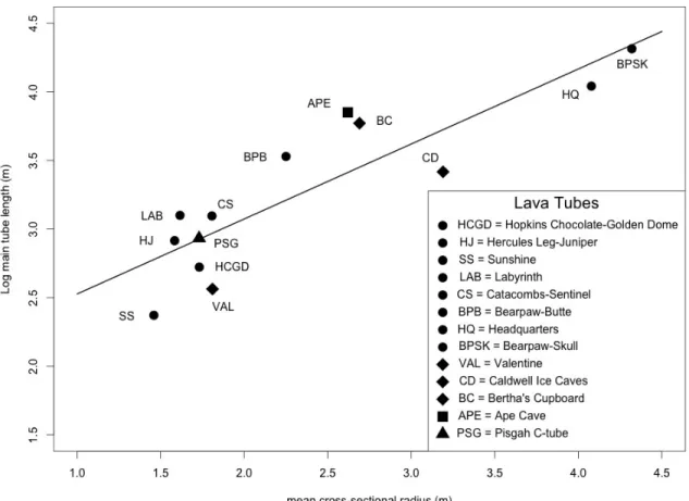
Tube length is positively correlated with both mean radius and aspect ratio (Figs. 8, 9). Additional length and radius data were obtained from previous three-dimensional mapping by the author of Valentine Cave in the basaltic andesite of Valentine Cave at Lava Beds National Monument, and the C-tube system at Pisgah Crater, San Bernardino County, California, and from preexisting maps of Caldwell Ice Caves and Bertha’s Cupboard Cave at Lava Beds (Waters et al., 1990), and Ape Cave at Mount St. Helens, Washington (Greeley and Hyde, 1971).
Elevation profiles for both master tubes are plotted in Figure 10. I calculated length-weighted average slopes for both master tubes by calculating the slope between successive data points, scaling these values by the distance between the points divided by the total tube length, and summing these weighted slopes (Table 1).
SS (n=35) HJ (n=305) HCGD (n=37) LAB (n=87) CS (n=99) HQ (n=59) BP−SK (n=30)
0
2
4
6
8
10
mean cross
−
sectional r
Figure 9 Aspect ratios for lava tube caves in the MC basalt (circles), and for tubes within other flows at Lava Beds National Monument, Mount St. Helens, and Pisgah Crater.
a b
Figure 10 Elevation profiles for the Headquarters (a) and Bearpaw-Skull (b) master tubes. The red lines are the segments used for thermal budget calculations.
0.3 0.4 0.5 0.6 0.7 0.8 0.9 1.0
1.5 2.0 2.5 3.0 3.5 4.0 4.5 aspect ratio
Log main tube length (m)
HJ LAB CS SS VAL HCGD PSG BC APE CD HQ BPSK
0 2000 4000 6000 8000 10000
1350 1400 1450 1500 1550 1600
horizontal distance (m)
ele
vation (m)
0 5000 10000 15000 20000
1250 1300 1350 1400 1450 1500 1550 1600
horizontal distance (m)
4.2 Rock Compositions
Whole rock major element compositions for samples collected during this study and from Donnelly-Nolan (2008) are in Table 2. Silica content in the MC basalt ranges from ~48.7-56.0 wt. %; in the Bearpaw-Skull master tube (samples M-2A and M-2), higher-SiO2 basaltic andesite erupted first, followed by lower-SiO2 high-alumina basalt.
Surface tubes and flow units proximal to Mammoth Crater have the highest wt.% SiO2,
and flow units distal to Mammoth Crater have lowest wt.% SiO2. In Hercules Leg–
Juniper Cave, roof rocks have higher SiO2 than a sample collected from a lava spring on
the floor representing the terminal lava flow within the tube as it drained and the residual lava solidified.
Mg variation diagrams of whole-rock compositions from the basalts of Mammoth Crater (Donnelly-Nolan, 2008) and Giant Crater (Baker et al., 1991) are shown in Figure 11. MC lavas are higher in SiO2 and lower in FeO, CaO, and TiO2, and have a smaller
26
Table 2 Whole rock major element analysis of Basalt of Mammoth Crater (normalized to 100 wt.%)
a Whole rock XRF analyses reported by Donnelly-Nolan (Donnelly-Nolan, 2008), LOI at 900° C b Analyses of rock standards for whole rock analyses performed for current study
c Non-normalized sums for new analyses Sample SiO2 TiO2 Al2O3 Fe2O3
tot
Mn O
Mg O
CaO Na2 O
K2O P2O5 Sumc LOI
HL-2 54.57 0.72 16.86 7.74 0.14 6.84 8.69 3.06 1.22 0.15 100.08 0.100
J-1 55.98, 0.71, 16.53, 7.57 0.13 6.53 8.15 3.01 1.27 0.11 99.82 0.80
J-N6 55.43 0.72 16.57 7.64 0.13 6.88 8.42 2.96 1.17 0.10 100.49 0.44 J-LS 54.13 0.73 16.85 7.91 0.14 7.05 8.99 2.96 1.10 0.14 99.92 0.05 SS-1 54.95 0.73 16.72 7.85 0.14 6.95 8.57 2.90 1.09 0.11 99.61 0.26
SS-3 54.56 0.75 17.11 7.96 0.14 6.84 8.55 2.84 1.12 0.14 99.70 0.74
M-1 53.86 0.77 17.08 8.24 0.14 6.95 8.74 2.99 1.10 0.11 100.38 0.59
M-2 50.43 0.85 17.59 9.29 0.16 8.15 10.08 2.80 0.52 0.14 100.57 -0.01
M-2A 54.79 0.75 16.76 7.93 0.14 6.91 8.40 2.99 1.23 0.11 101.08 0.10 BP-1 51.73 0.80 17.37 8.78 0.15 7.82 9.55 2.92 0.77 0.12 100.18 -0.13 CJ-1 53.32 0.78 17.08 8.31 0.14 7.27 8.87 3.03 1.06 0.12 100.55 0.01
646Ma 54.78 0.69 17.01 7.75 0.13 6.64 8.50 3.04 1.36 0.11 98.76 0.64
982Ma 48.78 0.83 17.98 9.67 0.16 8.89 10.53 2.73 0.32 0.11 100.66 -
990Ma 49.67 0.86 17.68 9.54 0.19 8.36 10.33 2.77 0.48 0.11 100.66 0.04
7 8 9 10
48
50
52
54
56
MgO wt. %
SiO
2
wt. %
7 8 9 10
0.2
0.4
0.6
0.8
1.0
1.2
1.4
MgO wt. % K2
O wt. %
7 8 9 10
8
9
10
11
12
MgO wt. %
CaO wt. %
7 8 9 10
7
8
9
10
11
MgO wt. %
Fe
2
O3
Figure 11 Mg variation plots of MC basalt and basalt of Giant Crater samples.
4.3 Petrography
Modal mineralogy and vesicle abundance are reported in Table 3. In all samples
plagioclase is the dominant mineral phase, with minor olivine and augite. Samples J-1
and J-LS have intergranular texture; all other samples have a vitreous groundmass.
Figure 12 Reversely zoned plagioclase xenocrysts in sample J-LS (field of view 1.7 mm wide).
7 8 9 10
16.0
16.5
17.0
17.5
18.0
18.5
MgO wt. % Al2
O3
wt. %
7 8 9 10
2.0
2.5
3.0
3.5
MgO wt. %
Na
2
O wt. %
7 8 9 10
0.0
0.5
1.0
1.5
MgO wt. %
TiO
2
wt. %
MC basalt (new)
MC basalt (Donnely−Nolan, 2008) basalt of Giant Crater group 1 (Baker, et al., 1991)
basalt of Giant Crater group 2
basalt of Giant Crater group 3
basalt of Giant Crater group 4
basalt of Giant Crater group 5
The plagioclase in every sample consists of two populations: small laths and
larger xenocrysts (Fig. 12). Semi-quantitative energy-dispersive X-ray spectrometry
indicates that the plagioclase xenocrysts are reversely zoned with An36-43 cores rimmed
by sieved plagioclase An46-57, covered by an An55 armor (Fig. 13). Similar xenocrysts
were observed in samples from Giant Crater (Baker et al., 1991).
Measured vesicle fractions range from 0.091 to 0.491, and are generally higher in
samples collected from the Bearpaw-Skull master tube. There does not appear to be any
correlation between silica content and vesicle fraction. The mean major and minor axes
for the ellipses of best fit for vesicles measured and the mean length of plagioclase
phenocrysts are reported in Table 4.
Table 3 Modal mineralogy, volume fraction of crystals, vesicles, and groundmass
Sample Plag Olv Aug Plag
xenoliths
Vesicles Groundmass Crystal fraction (rock including vesicles) HL-2 0.119 0.016 0.005 0.017 0.243 0.600 0.157 J-1 0.256 0.001 groundmass 0.030 0.206 0.507 0.287 J-LS 0.262 0.018 groundmass 0.019 0.230 0.471 0.299 SS-3 0.139 0.048 0.021 0.012 0.330 0.450 0.220
M-1 0.136 0.016 0.012 0.022 0.376 0.438 0.186
M-2 0.145 0.016 0.014 0.002 0.380 0.443 0.177
M-2A 0.072 0.008 0.004 0.013 0.491 0.410 0.099 BP-1 0.140 0.027 0.002 0.018 0.377 0.436 0.187 CJ-1 0.249 0.062 0.005 0.028 0.091 0.564 0.345
Table 4 Size comparison between plagioclase phenocrysts and vesicles
Sample Vesicle mean major axis (mm) Vesicle maximum major axis (mm) Vesicle mean minor axis (mm) Vesicle maximum minor axis (mm)
Mean length of ten largest plagioclase crystals (mm)
HL-2 0.8 16.7 0.4 4.0 0.22
J-1 0.4 7.3 0.2 4.8 0.25
J-LS 0.4 16.9 0.2 7.6 0.18
SS-3 0.9 18.2 0.5 7.0 0.26
M-1 1.7 16.3 1.0 6.7 0.30
M-2 0.6 18.9 0.3 10.9 0.34
M-2A 0.6 14.3 0.4 6.1 0.11
Figure 13 Backscattered electron image of a reversely zoned plagioclase xenocryst in sample J-N6 from
Hercules Leg-Juniper Cave. Semi-quantitative analysis indicates that the core is An36-43, surrounded by a
sieved An46-57 plagioclase rimmed by An55 plagioclase armor.
4.4 Viscosity modeling
Estimated melt and effective viscosities for anhydrous and wet (1 wt. % H2O)
compositions are given in Table 5. In every sample the vesicles are larger than the mean
length of the ten largest plagioclase crystals in that sample. Consequently effective
viscosities were calculated using Harris and Allen’s (2008) first case where vesicle size >
crystal size.
Isothermal melt viscosities decrease as SiO2 content decreases (Fig. 14). This
trend generally holds for effective viscosities as well. The addition of 1 wt.% H2O
An36%43'core' An55'armor'
reduces melt and effective viscosities by approximately one order of magnitude (Fig.
14b). Samples with a crystal fraction greater than the vesicle fraction have effective
viscosities greater than the melt viscosity, and show an expanded range of effective
viscosities over temperatures of 1080-1160 °C when compared with the corresponding
range of melt viscosities. Conversely, samples with a crystal fraction less than the vesicle
fraction show an effective viscosity less than or sub-equal to the melt viscosity, and show
a contracted range in effective viscosities over 1080-1160 °C relative to the
corresponding range in melt viscosities. These petrographic and temperature dependent
viscosity ranges are plotted vs. SiO2 content in Figure 14.
Table 5 Calculated melt and effective viscosities (Pa-s) of dry and wet (1 wt. % H2O) of MC basalt samples
Sample 1080
°C& 1090 °C& 1100 °C& 1110 °C& 1120 °C 1130
°C 1140 °C 1150 °C 1160 °C
BP-1 ηmelt dry 741 602 478 389 315 257 211 174 144 BP-1 ηeff dry 611 497 394 321 259 212 174 143 119 BP-1 ηmelt wet 75 64 54 46 40 34 29 25 22 BP-1 ηeff wet 62 53 45 38 33 28 24 21 18 CJ-1 ηmelt dry 1445 1148 912 741 596 485 397 326 269 CJ-1 ηeff dry 3607 2865 2276 1850 1489 1212 991 814 672 CJ-1 ηmelt wet 121 109 93 79 67 57 49 42 36 CJ-1 ηeff wet 304 273 232 198 168 143 123 106 92
a
0 1000 2000 3000 4000 5000 6000
50 51 52 53 54 55 56
Viscosity (Pa−s)
SiO 2 wt. % | | | | | | | | | | | | | | | | | | | | | | | | | | | | | | | | | | | | | | || || ||| | | | | | | | || | | | | || || | | | | | | | | | |
Projected effective viscosity range (1080−1160oC)
Melt viscosity 1160oC
Melt viscosity 1080oC HL−2, SS−3
J−1
J−LS M−1
M−2
M−2A
BP−1
CJ−1
b
c
Figure 14 (a) Calculated melt and effective viscosities for anhydrous MC basalt samples, and (b) calculated melt and effective viscosities for MC basalt samples containing 1 wt.% H2O, plotted as a
function of SiO2 wt.%. The SiO2 axes on (a) and (b) use the anhydrous SiO2 values for each sample.
Viscosities were calculated for a temperature range of 1080-1160 °C. Effective viscosities for (a) and (b) are plotted as projections of viscosity versus temperature curves onto the viscosity-SiO2 plane looking
down the temperature axis. (c) An example using sample J-1 (1 wt.% H2O) of the projection method used
0 100 200 300 400 500
50 51 52 53 54 55 56
Viscosity (Pa−s)
SiO 2 wt. % | | | | | | | | | | | | | | | | | | | | | | | | | | | | | | | | | | | | | || || || || | | | | | | | | | | | | | | | || | | | | | | | | | |
HL−2, SS−3
J−1
J−LS
M−1
M−2
M−2A
BP−1
CJ−1
1160oC 1080oC
100 200 300 400 500
1080
1100
1120
1140
1160
viscosity (Pa−s)
temper
ature (
oC)
4.5 Thermal modeling
The results of the thermal budget models for the Headquarters and Bearpaw-Skull
master tubes, and the Headquarters near-surface distributary tubes are given in Tables 6
and 7. All cumulative cooling values are below the 50 °C cooling threshold used by
Keszthelyi to the estimate cooling-limited length of tube-fed lava flows. None of the lava
35
Table 6 Calculated cooling for Headquarters and Bearpaw-Skull master tubes (number of skylights = 2/km)
Lava tube segment
Slope Length (m)
Lava density (kg/m3)
H2O wt.% Temperature (°C) Effective viscosity (Pa s) Thermal erosion rate (m/s) Effusion rate (m3/s)
36
HQ 10 -0.016 1011 1560 1 1150.4 107 9.7x10⁻⁷ 242 57708 0.0 0.0 4416
Lava tube segment
Slope Length
(m)
Lava density (kg/m3)
H2O
wt.% Temperature (°C) Effective viscosity (Pa s) Thermal erosion rate (m/s) Effusion rate (m3/s)
Viscous dissipation (W/m) !" !" (°C/km) Cumulative cooling (°C) Cooling-limited length of last segment (km)
HQ 1 -0.029 961 2600 1 1150.0 107 1.0x10⁻⁶ 752 556149 0.1 -0.1 -
HQ 2 -0.021 993 2600 1 1150.1 107 9.0x10⁻⁷ 533 278804 0.0 0.0 -
HQ 3 -0.025 969 2600 1 1150.1 107 9.7x10⁻⁷ 651 416043 0.1 -0.1 -
HQ 4 -0.047 942 2600 1 1150.2 107 1.2x10⁻⁶ 1222 1468640 0.2 -0.1 -
HQ 5 -0.062 984 2600 1 1150.3 107 1.3x10⁻⁶ 1606 2533139 0.2 -0.2 -
HQ 6 -0.052 1000 2600 1 1150.5 107 1.2x10⁻⁶ 1342 1771403 0.2 -0.2 -
HQ 7 -0.026 984 2600 1 1150.7 107 9.8x10⁻⁷ 685 460878 0.1 -0.1 -
HQ 8 -0.005 1002 2600 1 1150.8 107 5.7x10⁻⁷ 134 17598 -0.1 0.1 -
HQ 9 -0.009 996 2600 1 1150.7 107 6.9x10⁻⁷ 242 57617 0.0 0.0 -
HQ 10 -0.016 1011 2600 1 1150.7 107 8.2x10⁻⁷ 404 160304 0.0 0.0 Infinity
BPSK 1 -0.018 2088 1560 0 1150.0 809 4.1x10⁻⁷ 47 13095 -0.3 0.6 -
BPSK 2 -0.019 1071 1560 0 1149.4 826 5.1x10⁻⁷ 48 13813 -0.3 0.3 -
BPSK 3 -0.065 1061 1560 0 1149.1 826 7.7x10⁻⁷ 163 161133 0.1 -0.1 -
BPSK 4 -0.027 2048 1560 0 1149.3 826 4.7x10⁻⁷ 70 29188 -0.1 0.3 -
BPSK 5 -0.021 2064 1560 0 1149.0 826 4.3x10⁻⁷ 54 17660 -0.2 0.5 -
BPSK 6 -0.018 2021 1560 0 1148.5 845 4.0x10⁻⁷ 43 11668 -0.3 0.6 -
BPSK 7 -0.015 2023 1560 0 1147.9 845 3.8x10⁻⁷ 36 8066 -0.4 0.8 -
BPSK 8 -0.009 2064 1560 0 1147.2 866 3.2x10⁻⁷ 22 2965 -0.7 1.4 -
BPSK 9 -0.014 2052 1560 0 1145.7 886 3.6x10⁻⁷ 33 6979 -0.4 0.9 -
BPSK 10 -0.001 2086 1560 0 1144.9 906 1.3x10⁻⁷ 2 17 -9.6 20.1 -
BPSK 11 -0.003 2036 1560 0 1124.8 1340 1.9x10⁻⁷ 5 204 -3.2 6.6 16
BPSK 1 -0.018 2088 2600 0 1150.0 809 3.4x10⁻⁷ 78 36376 -0.1 0.2 -
BPSK 2 -0.019 1071 2600 0 1149.8 826 4.3x10⁻⁷ 80 38371 -0.1 0.1 -
BPSK 3 -0.065 1061 2600 0 1149.8 826 6.5x10⁻⁷ 272 447592 0.2 -0.2 -
BPSK 4 -0.027 2048 2600 0 1150.0 809 4.0x10⁻⁷ 118 82782 0.0 0.0 -
BPSK 5 -0.021 2064 2600 0 1150.0 809 3.6x10⁻⁷ 92 50087 0.0 0.1 -
BPSK 6 -0.018 2021 2600 0 1149.9 809 3.4x10⁻⁷ 76 33853 -0.1 0.2 -
BPSK 7 -0.015 2023 2600 0 1149.7 826 3.2x10⁻⁷ 62 22922 -0.1 0.3 -
BPSK 8 -0.009 2064 2600 0 1149.5 826 2.7x10⁻⁷ 38 8634 -0.2 0.5 -
37
Lava tube segment
Slope Length
(m)
Lava density (kg/m3)
H2O
wt.% Temperature (°C) Effective viscosity (Pa s) Thermal erosion rate (m/s) Effusion
rate (m3/s) Viscous dissipation
(W/m) !" !" (°C/km) Cumulative cooling (°C) Cooling-limited length of last segment (km)
BPSK 10 -0.001 2086 2600 0 1148.7 826 1.1x10⁻⁷ 3 51 -3.6 7.5 -
BPSK 11 -0.003 2036 2600 0 1141.2 971 1.8x10⁻⁷ 10 781 -1.0 2.0 51
BPSK 1 -0.018 2088 1560 1 1150.0 107 8.0x10⁻⁷ 356 99011 0.0 0.0 -
BPSK 2 -0.019 1071 1560 1 1150.0 107 1.0x10⁻⁶ 369 106635 0.0 0.0 -
BPSK 3 -0.065 1061 1560 1 1150.1 107 1.5x10⁻⁶ 1261 1243888 0.2 -0.2 -
BPSK 4 -0.027 2048 1560 1 1150.3 107 9.2x10⁻⁷ 537 225321 0.1 -0.1 -
BPSK 5 -0.021 2064 1560 1 1150.4 107 8.5x10⁻⁷ 417 136330 0.0 -0.1 -
BPSK 6 -0.018 2021 1560 1 1150.5 107 8.0x10⁻⁷ 343 92143 0.0 0.0 -
BPSK 7 -0.015 2023 1560 1 1150.5 107 7.5x10⁻⁷ 285 63702 0.0 0.0 -
BPSK 8 -0.009 2064 1560 1 1150.5 107 6.3x10⁻⁷ 175 23902 -0.1 0.1 -
BPSK 9 -0.014 2052 1560 1 1150.4 107 7.4x10⁻⁷ 272 57791 0.0 0.0 -
BPSK 10 -0.001 2086 1560 1 1150.3 107 2.7x10⁻⁷ 13 140 -1.2 2.4 -
BPSK 11 -0.003 2036 1560 1 1147.9 110 4.3x10⁻⁷ 56 2480 -0.3 0.6 183
BPSK 1 -0.018 2088 2600 1 1150.0 107 6.8x10⁻⁷ 593 275029 0.0 -0.1 -
BPSK 2 -0.019 1071 2600 1 1150.1 107 8.5x10⁻⁷ 615 296208 0.0 0.0 -
BPSK 3 -0.065 1061 2600 1 1150.1 107 1.3x10⁻⁶ 2102 3455243 0.2 -0.2 -
BPSK 4 -0.027 2048 2600 1 1150.4 107 7.8x10⁻⁷ 895 625892 0.1 -0.2 -
BPSK 5 -0.021 2064 2600 1 1150.5 107 7.1x10⁻⁷ 696 378693 0.1 -0.1 -
BPSK 6 -0.018 2021 2600 1 1150.6 107 6.7x10⁻⁷ 572 255952 0.0 -0.1 -
BPSK 7 -0.015 2023 2600 1 1150.7 107 6.3x10⁻⁷ 476 176950 0.0 -0.1 -
BPSK 8 -0.009 2064 2600 1 1150.8 107 5.4x10⁻⁷ 292 66654 0.0 0.0 -
BPSK 9 -0.014 2052 2600 1 1150.8 107 6.2x10⁻⁷ 453 160530 0.0 0.0 -
BPSK 10 -0.001 2086 2600 1 1150.8 107 2.3x10⁻⁷ 22 390 0.5 1.0 -
38
Table 7 Calculated cooling for near-surface tubes (T0 = 1150 °C)
Lava tube Slope Length (m) Number Skylights Lava density kg/m3
H2O
wt.% Effective viscosity (Pa s) Thermal erosion rate (m/s) Effusion rate (m3/s)
!" !" (°C/km) Cumulative cooling (°C) Cooling- limited length (km) SS -0.071 235 2 1560 0 513 1.5×10⁻⁶ 4 -2.4 0.6 21
SS -0.071 235 2 1560 1 63 3.1×10⁻⁶ 31 -0.1 0.0 474 SS -0.071 235 2 2600 0 513 1.3×10⁻⁶ 6 -0.8 0.2 60
SS -0.071 235 2 2600 1 63 2.6×10⁻⁶ 51 -0.1 0.0 ∞
HJ -0.035 823 9 1560 0 528 8.0×10⁻⁷ 3 -4.4 3.7 11
HJ -0.035 823 9 1560 1 63 1.6×10⁻⁶ 21 -0.4 0.4 113 HJ -0.035 823 9 2600 0 528 6.7×10⁻⁷ 4 -1.7 1.4 29
HJ -0.035 823 9 2600 1 63 1.4×10⁻⁶ 35 -0.1 0.1 461
HCGD -0.046 528 1 1560 0 528 1.0×10⁻⁶ 3 -1.6 0.8 32
HCGD -0.046 528 1 1560 1 63 2.1×10⁻⁶ 39 -0.1 0.0 773 HCGD -0.046 528 1 2600 0 528 8.5×10⁻⁷ 8 -0.6 0.3 87 HCGD -0.046 528 1 2600 1 63 1.7×10⁻⁶ 65 0.1 0.0 ∞
LAB -0.056 1258 3 1560 0 528 8.1×10⁻⁷ 4 -1.6 2.1 31
LAB -0.056 1258 3 1560 1 63 1.6×10⁻⁶ 37 0.0 0.1 1304
LAB -0.056 1258 3 2600 0 528 6.8×10⁻⁷ 7 -0.6 0.7 87 LAB -0.056 1258 3 2600 1 63 1.4×10⁻⁶ 61 0.1 -0.1 ∞ CS -0.045 1246 0 1560 0 528 7.6×10⁻⁷ 4 -1.8 2.3 28 CS -0.045 1246 0 1560 1 63 1.5×10⁻⁶ 30 -0.1 0.1 527 CS -0.045 1246 0 2600 0 528 6.4×10⁻⁷ 6 -0.7 0.9 73
5. Discussion
5.1 Compositional Zonation of MC Basalt
The compositional trends on the Mg-variation diagrams for the basalts of
Mammoth and Giant Craters are similar, but the MC basalt lacks the compositional gap
(Fig. 11) attributed to a pause in eruptive activity at Giant Crater (Baker et al., 1991), and
lacks compositions over 9 wt.% MgO. Stratigraphic relationships between flow units in
the Bearpaw-Skull master tube (samples M-2A and M-2) and Hercules Leg-Juniper Cave
(samples J-1, HL-2, and J-LS) indicate that the MC basalt progressed from basaltic
andesite (~56 wt.% SiO2) to basalt (~50 wt.% SiO2) as hypothesized by Donnelly-Nolan
(2011). ThusSiO2 can be used as a proxy for time, allowing for relative dating of flow
units and lava tubes.
Samples collected from the Bearpaw-Skull master tube span nearly the entire
range of SiO2 contents found in the MC basalt, suggesting that this tube was active during
the entire duration of the Mammoth Crater eruption. The Headquarters and
Bearpaw-Skull master tubes were fed from the same location in the former lava lake, therefore it is
likely that samples collected from Bearpaw-Skull represent lava compositions from
Headquarters.
The relatively high SiO2 content and narrow range of compositions observed in
samples from the near-surface system surrounding the Headquarters master tube indicates
that these tubes were formed relatively early in Mammoth Crater eruption, and that active
formation of these tubes was caused by blockage of the master tube, then the blockage
may have been cleared by thermal and mechanical erosion during the time it took for the
MC basalt to change from 55.9 to 54.1 wt.% SiO2.
5.2 Lava viscosity
Lava is a mixture of a silicate melt, crystals, and vesicles. Viscosity strongly
controls the transport properties and eruptive behavior of lava (Giordano and Dingwell,
2002; Giordano et al., 2008; Harris and Allen, 2008; Vona et al., 2011). The composition
of the melt phase (particularly SiO2 and H2O), the size and volume fraction of crystals
and vesicles, and temperature control the effective viscosity of lava.
Silicate-melt viscosity is strongly and inversely controlled by temperature.
Because the eruption temperature of the MC basalt is unknown, I calculated melt
viscosities for a range of 1080-1160 °C. These values bracket the range of lava
temperatures recorded through skylights in lava tubes in Hawaii (1130-1165 °C;
Pinkerton et al., 2002), the temperatures (1157-1131 °C) at which clinopyroxene first
crystallized during experiments on compositionally similar high-alumina basalts from
Etna and Stromboli (Vona et al., 2011), and the 50 °C decrease in lava temperature used
to determine the cooling-limited lengths of lava tubes in the thermal models of Keszthelyi
(1995).
High-pressure experiments on basalts in the Mount Shasta region (Grove et al.,
2001) indicate pre-eruptive H2O contents of ~1-8 wt.% that vary directly with SiO2
content. Analyses of OH concentrations in plagioclase from tholeiitic basalts and
andesites erupted at Izu-Oshima volcano show a decrease in dissolved H2O content from
surface (Hamada, 2011). Additional degassing occurs during lava storage in lava lakes
(Tazieff, 1994); therefore an upper limit of 1 wt.% H2O is reasonable for calculating
hydrous melt viscosity.
The decrease in SiO2 content during the eruption of the MC basalt resulted in a
general decrease in effective viscosity over time, regardless of temperature variations
(Fig. 14). Uncertainties in the H2O content and temperature of the lava during the course
of eruption limits inferences about lava rheology.
5.3 Lava tube morphology
The cross-sectional data for lava tubes within the MC basalt shows a difference in
the mean radius of master tubes and distributary tubes. Observations of Hawaiian lava
tubes show that tubes with smaller cross-sectional radii are immature, and active for a
shorter time compared to larger radius master tubes that are active for an extended time
(Cooper and Kauahikaua, 1992). Thermal and mechanical erosion of the floor and
roof-collapse during active flow increase the tube radius (Keszthelyi, 1995); consequently
tubes that are active longer tend to have larger mean cross-sectional radii. The aspect
ratio of a lava tube can be used a rough indicator of its maturity, because thermal and
mechanical erosion also tend to increase the aspect ratio. The aspect ratios of lava tubes
in this study show a positive correlation between aspect ratio and length (Fig. 9). These
results support a shorter duration of flow within distributary tubes and a longer duration
of flow within master tubes.
The lava tubes studied show a positive correlation between length and mean
radius. This suggests a mechanism relating these parameters. I propose that this trend
flows (Fig. 15; Walker, 1973; Malin, 1980; Pinkerton and Wilson, 1994; Harris and
Rowland, 2009). Observations of Hawaiian channel-fed flows show that most are
cooling-limited (Pinkerton and Wilson, 1994). Lava channels lose heat more efficiently
through radiation and air convection than do lava tubes. Lava effusion rate is another
important parameter governing the rate of cooling in channel- and tube-fed flows. Flows
with higher effusion rates lose less heat with distance than flows with lower effusion
rates. Harris and Rowland (2009) noted that the length-effusion rate relationship only
holds for channel-fed flows that achieve their cooling-limited length.
Pinkerton and Wilson (1994) argued that tube-fed flows should be considered
separately from channel-fed flows. This conclusion is reasonable given the lack of a
length-effusion rate relationship for tube-fed flows (Pinkerton and Wilson, 1994; Harris
and Rowland, 2009). Lava tubes are enclosed, limiting radiation and convection to
skylights. This effectively insulates the lava from heat loss over the length of the tube
(Swanson, 1973). Insulation permits low-effusion rate flows to travel longer distances
with less cooling than channel-fed flows. This causes tube-fed flow lengths to deviate
from the length-effusion rate relationship exhibited by lava channels (Pinkerton and
Wilson, 1994; Harris and Rowland, 2009). Harris and Rowland (2009) noted that most
tube-fed flows that develop master tubes are volume-limited, where the supply of lava to
the tube ceases before the cooling-limited length is achieved.
I calculatedtube-full effusion rates using the Hagen-Poiseuille equation
(Sakimoto et al., 1997) for lava tubes in the MC basalt, Valentine Cave, Bertha’s
Cupboard Cave, Caldwell Ice Caves, Ape Cave, and C-Tube. I calculated effective
methodology used for samples from the MC basalt (see Appendices A.4 and A.5 for
compositional and petrographic data respectively). I accounted for uncertainties in
effective viscosity due to unknown temperatures and water contents by using a
temperature range of 1080-1160 °C, and water contents of 0 and 1 wt.% for effusion rate
calculations.
The lengths of these lava tubes and associated trench chains are plotted vs. the
calculated tube-full effusion rates in Figure 15. There is a positive correlation between
the tube length and estimated volumetric flow rate paralleling that noted above for
channel-fed flows. The effusion rate vs. flow length data from Figure 1 of Pinkerton and
Wilson (1994) is plotted with the data from this study. A comparison of these data shows
that the calculated effusion rates vs. lengths for lava tubes in this study plot exclusively
within the field of channel-fed flows regardless of uncertainties in temperature, water
content, and density.
a
-1 0 1 2 3 4
2.0 2.5 3.0 3.5 4.0 4.5 5.0
Effusion rate (m3/s)
Lo g flo w le ng th (m) | | | | | | | | | | | | | | | | | | | | | | | |
Basalt of Mammoth Crater tubes
Other Lava Beds tubes
C-tube Pisgah Crater
Ape Cave Channel-fed flows
b
c
-1 0 1 2 3 4
2.0 2.5 3.0 3.5 4.0 4.5 5.0
Log effusion rate (m3/s)
Lo g flo w le ng th (m) | | | | | | | | | | | | | | | | | | | | | | | |
-1 0 1 2 3 4
2.0 2.5 3.0 3.5 4.0 4.5 5.0
Log effusion rate (m3/s)
d
Figure 15 Measured lava tube length vs. estimated tube-full effusion rates compared with channel and tube-fed flow observations (circles and asterisks) from Fig. 1 of Pinkerton and Wilson (1994). Effusion rates for lava tubes in this study were calculated using the Hagen-Poiseuille equation. Viscosities were calculated for anhydrous low (a) and high (b) density lavas, and hydrous (1 wt.% H2O) low (c) and high (d)
density lavas. The length of the bars represents the range of effusion rates resulting from temperature dependent viscosity variation from 1080-1160 °C.
It is possible that the near-surface tubes considered in the current study were
initially channel-fed flows that roofed-over late in their development, and that large
segments of the master tubes were open channels. Late-stage roofing-over of segments of
channel-fed flow may cause lava tubes to exhibit the length-effusion rate relationship that
channel-fed flows have. If this true then the thermal models for mature lava tubes
developed by Keszthelyi (1994) do not adequately describe the thermal budget of the lava
tubes considered in this study. Because the Hagen-Poiseuille equation was used to
calculate effusion rates, the values calculated represent tube-full conditions that would
have occurred immediately after roofing-over of a channel-fed flow.
The skylights in Sunshine Cave (Fig. 16) exhibits a jumbled structure suggesting
-1 0 1 2 3 4
2.0 2.5 3.0 3.5 4.0 4.5 5.0
Log effusion rate (m3/s)
(Greeley and Hyde, 1971). Greeley and Hyde (1971) noted that such tubes likely form on
relatively steep slopes and tend to form arched roofs such as the one in Sunshine Cave.
Figure 16 A skylight in Sunshine Cave showing the tube lining and re-melt features on the interior of the tube, and layering between the tube ceiling and the surface. Note the arched roof and jumbled appearance of the rock exposed in the skylight. These features are indicative of a lava tube formed by the roofing over of a channel-fed flow (Greeley and Hyde, 1971).
Roofing-over of a channel-fed flow is likely the case for the Pisgah Crater C-tube
system where the tube comprises three flow units separated by relict pahoehoe flow
surfaces. The poor preservation of lava tube roofs and walls at Pisgah Crater has removed
tube-lining features such as re-melt glazing and lavacicles, exposing flow-unit
stratigraphy from the floor to the roof of the lava tube. Two mechanisms of lava tube
formation in the Ape Cave system were noted by Greeley and Hyde (1971); some tube
sections were formed by the accretion of lava spatter from turbulent channel-fed flows
shear planes within a solidifying flow, indicated by smooth layering of flow units in
skylights.
Considering that the Headquarters and Bearpaw-Skull master tubes exhibit the
same length-radius relationship as roofed-over channels like Ape Cave and the C-tube, it
is likely that these master tubes had significant segments of channel-confined flow when
they were active. The degree to which these master tubes were channel-fed is unknown
given the state of collapse along many segments of them.
5.4 Thermal Modeling
Thermal model results for the Headquarters and Bearpaw-Skull master tubes and
the Headquarters near-surface tubes indicate that water content plays a significant role in
determining the cooling-limited length of a lava tube (Tables 6 and 7). Increasing the
dissolved water content of the lava decreases the viscosity, causing the effusion rate to
increase. This reduces the amount of cooling per unit distance along the length of a tube.
In master tube segments with steep slopes, viscous dissipation increases lava temperature
for low-viscosity hydrated lava, effectively maintaining lava viscosity and volumetric
flow rate over the length of the tube, whereas temperature decreases for higher-viscosity
anhydrous lava.
All of the lava tubes modeled fall short of their tube-fed cooling-limited lengths,
indicating that either the tubes are volume-limited in length, or that the lava flow was not
exclusively tube-fed. It is important to note that the thermal budget model of Keszthelyi
(1995) is only valid for mature tube-fed flows. As such the calculated cumulative cooling
values for lava tubes in this study only apply to fully developed tube-fed flow.
tubes in this study and the channel-fed flows from Pinkerton and Wilson (1994), it is
likely that the thermal budget results reported here are not valid for estimating the
cooling-limited lengths for the lava tubes studied.
5.5 Significance for evaluating extra-terrestrial lava tube caves
Lava tube skylights form by roof collapse (Peterson and Swanson, 1974) and can
attain a maximum width equal to that of the lava tube. The widths of skylights and
collapse trenches can be used to estimate the radius of a lava tube. The length of chains of
skylights and collapse trenches can be used to estimate lava tube length. Both of these
parameters can be measured using remote-sensing techniques. The positive correlation
between lava tube lengths and radii observed in this study is independent of composition
and petrographic texture, and can be used as a means for evaluating whether or not a lava
6. Conclusions
The eruption of the MC basalt initiated with the effusion of ~56 wt.% SiO2
basaltic andesite and progressed to ~50 wt.% SiO2 basalt during the course of the
eruption. This progression towards more mafic lava caused a general decrease in the melt
and effective viscosity of the lava over the course of the eruption, and can be used as a
means to relatively date flow units within the MC basalt.
There is a positive correlation between lava tube length and mean radius. This
correlation is independent of the compositional and petrographic character of the host
rock. Because the effusion rate in a lava tube is proportional to the fourth power of the
cross-sectional radius, the length-radius correlation found for lava tubes in this study
reflects the length vs. effusion rate relationship.
This study has shown that by using a combination of three-dimensional mapping
of extinct lava tubes, viscosity modeling, and thermal modeling it is possible to evaluate
whether a tube formed as a: (1) volume-limited lava tube formed by shear planes within a
cooling lava flow (in which case no length vs. radius relationship would be expected), (2)
a cooling-limited lava tube formed by shear planes in a cooling lava flow (the lava tube
would be approximately near its estimated cooling limited length), or (3) by means of the
roofing-over of a cooling-limited channel-fed flow (the length vs. calculated effusion rate