ANALYSIS OF THIN FILMS RELATED TO FLOWS IN CYLINDRICAL GEOMETRIES
Sterling Swygert
A dissertation submitted to the faculty at the University of North Carolina at Chapel Hill in partial fulfillment of the requirements for the degree of Doctor of Philosophy in the Department of
Mathematics in the College of Arts and Sciences.
Chapel Hill 2019
c
2019
ABSTRACT
Sterling Swygert: Analysis of Thin Films Related to Flows in Cylindrical Geometries
(Under the direction of Jeremy L. Marzuola)
Motivated by models for thin films coating cylinders in two physical cases proposed in [1] and [2], we analyze the dynamics of corresponding thin film models. The models are governed by nonlinear, fourth-order, degenerate, parabolic partial differential equations. We prove, given positive and suitably regular initial data, the existence of weak solutions in all length scales of the cylinder, where all solutions are only local in time. We also prove that given a length constraint on the cylinder, long-time and global in time weak solutions exist. This analytical result is motivated by numerical work on related models of Reed Ogrosky [3] in conjunction with the works [4, 5, 6, 7].
ACKNOWLEDGEMENTS
I would first like to thank my parents, Lisa and Donnie, for supporting me while I have been working diligently on this project. Thank you to Felix, Otto, Rachel, and Wally for keeping me sane at home and to my classmates for keeping me sane at school.
I am grateful for the guidance and advice given by Dr. Jeremy Marzuola throughout the work on this thesis. His insight, encouragement, and support have been invaluable. Thank you also to Dr. Roberto Camassa, Dr. Roman Taranets, and Dr. Reed Ogrosky for the opportunity to collaborate and learn from them in their various areas of expertise. Thank you also to the committee member Dr. Michael Taylor for being willing to examine and critique my work.
TABLE OF CONTENTS
LIST OF FIGURES . . . viii
CHAPTER 1: INTRODUCTION . . . . 1
CHAPTER 2: EXISTENCE OF NON-NEGATIVE WEAK SOLUTIONS . . . . 5
2.1 Model I Preliminaries . . . 5
2.1.1 Functionals . . . 5
2.1.2 Model I Energy Identities . . . 6
2.2 Model I Energy Estimates . . . 8
2.2.1 Local in Time Estimates . . . 8
2.2.2 Long-time Estimates on Ω⊂ −π 2, π 2 . . . 9
2.2.3 Hölder Continuity of{hε}ε>0 . . . 12
2.3 Weak Solutions to Model I . . . 16
2.4 Non-Negativity of Solutions to Model I . . . 19
2.5 Model II . . . 23
2.5.1 Local in Time Theory . . . 23
2.5.2 Global in Time Estimates on Ω⊂ −π 2, π 2 . . . 24
2.6 Extending the Results and Future Work . . . 27
CHAPTER 3: ANALYSIS OF TRAVELING WAVES . . . . 29
3.1 Traveling Waves in Model I . . . 29
3.1.1 Preliminaries . . . 29
3.1.2 Traveling Waves with Perturbation by Viscosity . . . 31
3.2 Traveling Waves in Model II . . . 42
3.2.1 Preliminaries . . . 42
3.3 Spectral Stability in Model I . . . 47
3.3.1 Preliminaries . . . 47
3.3.2 Model I Constant Coefficient Problem . . . 48
3.3.3 Perturbation of Model I Constant Coefficient Problem byεsinx/T . . . 49
3.3.4 Perturbation WhenQ−c=O(εα), α≥1 . . . 55
3.4 Spectral Stability in Model II . . . 57
3.4.1 Preliminaries . . . 57
3.4.2 Model II Constant Coefficient Problem . . . 58
3.4.3 Perturbation of Model II Constant Coefficient Problem byεsinx/T . . . 58
3.4.4 Perturbation When 2Q2−c=O(εα), α≥1 . . . 63
CHAPTER 4: CONCLUSIONS . . . . 65
LIST OF FIGURES
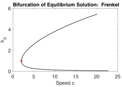
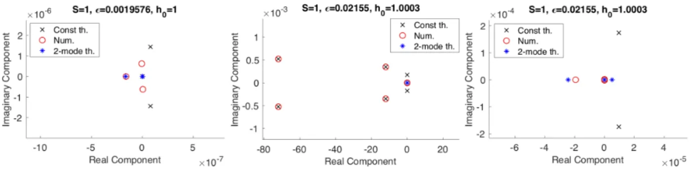
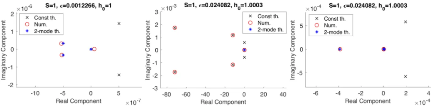
3.1 Family of equilibrium solutions shown in c−h0 space for (3.1), in collaboration with H.R. Ogrosky. A red ×represents a Hopf bifurcation. . . 31 3.2 A comparison of the amplitude, the background, and period of the numerically
computed solutions and the asymptotic solutions, in collaboration with H.R. Ogrosky. 40 3.3 Family of equilibrium solutions shown inc−h0 space for (3.51), in collaboration with
H.R. Ogrosky. A red ×represents a Hopf bifurcation. . . 43 3.4 A comparison of the amplitude, the background, and period of the numerically
computed solutions and the asymptotic solutions, in collaboration with H.R. Ogrosky. 46 3.5 A comparison of the eigenvalues of LK,c,eq comparison to the numerically computed
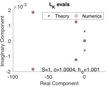
eigenvalues ofLK,c, in collaboration with H.R. Ogrosky. . . 49
3.6 A comparison of the numerically computed eigenvalues of LK,c with the eigenvalues
of the higher order perturbed operator ˜LK,c, in collaboration with H.R. Ogrosky. . . 56
3.7 A comparison of the numerically computed eigenvalues of LF,c with the eigenvalues
CHAPTER 1 Introduction
The analysis of liquid films is an area of mathematical research that has many applications, ranging from biological systems to engineering and has been a rich area of research over the last three decades. Generically, the films have one free boundary whose evolution is determined by the relationship between external forces and the surface tension of the free surface itself. Many modeling and numerical studies have been done in order to understand these flows in different parameters and geometrical setups. In particular [9] and [10] study films along an inclined plane and [11],[12],[5] consider films in the exterior or interior of vertically oriented tubes. The most significant physical difference between these two geometries is the free surface’s azimuthal curvature dictating the surface stress in the cylindrical setting. The interior case of the cylindrical geometry is studied extensively in [7]. A specific class of the films, called thin films, exploit the ratio between the thicknesses of the film and the cylinder. In [11], an evolution equation is derived for a thin film coating either the outside or the inside of a cylinder. This model was further studied in [2] and is explained in greater detail below. Thin films equations have also been studied in the frameworks of the generalized Kuramoto-Sivashinsky equation and the Cahn-Hilliard equation [13],[14].
Much work in the area has drawn on the machinery developed in [15], where the equation
ht+ (f(h)hxxx)x = 0, f(h) =f0(h)|h|n, 0< f0∈C1+α(R1), α∈(0,1), and n≥1 (1.1)
also be seen in [18]. A comprehensive discussion of the relationship between scaling properties and singularity formation can be found in [19].
Though there has been some work done in more general settings [20], thin films coating a cylinder have been studied extensively. Eres, Schwartz, and Weidner provided models and numerical work for a stationary, horizontally oriented cylinder in the presence of gravity [21]. Aside from modeling and numerical work, much analytic progress has been made by Chugunova, Pugh, and Taranets. For instance, they have studied the dynamics of a thin film on the exterior surface of a horizontally oriented cylinder rotating about it’s axis of symmetry and provided arguments for long-time existence of weak solutions [22],[23],[24].
In this dissertation, we study the dynamics of an incompressible thin fluid film on the exterior of a cylinder. In particular we consider two specific one dimensional models. The first model (Model I), derived in [1], is given by the initial boundary value problem
ht=−hhx−Sh3(hx+hxxx)x inQT,
h(x,0) =h0(x)∈H1(Ω),
∂xjh(−a,·) =∂xjh(a,·) for t∈(0, T), j = 0,1,2,3,
(1.2)
where Ω = (−a, a) is a bounded interval in R and QT = Ω×(0, T). The equation models the
situation in which the cylinder is horizontally oriented, a horizontally directed air flow is present without gravity, and the cylinder is fully coated so that the only free boundary is that where the surface of the fluid meets the air. Here,h is the thickness of the film with initial value h0 and x is the longitudinal position. Model II, derived in [2], is given by the initial boundary value problem
ht=−2h2hx−S
h3(hx+hxxx)
x inQT,
h(x,0) =h0(x)∈H1(Ω),
∂xjh(−a,·) =∂xjh(a,·) for t∈(0, T), j = 0,1,2,3.
(1.3)
and the first terms on the right hand sides represent the forces acting on the films, e.g., air flow in Model I and gravity in Model II. In the following sections, we provide local in time existence of weak solutions to both Model I and Model II. When Ω ⊂ −π2,π2
,we prove the existence of long-time weak solutions to Model I and global in time weak solutions to Model II. Furthermore, in all cases, we prove non-negativity property, i.e. positive initial conditions yields non-negative solutions. Schematic diagrams of each model and respective coordinates can be found in [1] and [2].
In chapter 2, we first prove the existence of weak solutions to Model I. In particular, we prove local in time existence of weak solutions with any bounded spatial domain and long-time existence of weak solutions when the spatial domain is restricted to Ω⊂ −π
2,
π
2
.The work for both the local in time and long-time solutions is broken up into four steps. First, we provide the definitions for functionals used throughout the paper and derive some straightforward identities in section 2.1. In section 2.2, we derive energy estimates for a regularized version of Model I and show control of the regularized solutions in different norms. In section 2.3, we define weak solutions and demonstrate that the limit of the solution to the regularized problem exists and satisfies this definition assuming non-negativity. Finally, we prove in section 2.4 that the limit is indeed nonnegative. In section 2.5, we examine Model II and give a brief description of how to prove the local in time existence of weak solutions. We then provide a proof for the existence of global in time solutions to Model II. Though many of the components of the proof are naturally analogous to those for Model I, the energy estimates are treated with a modified approach and are given in details. Finally, in section 2.6 we discuss future work in this analysis, including natural extensions of the arguments found here to long-wave models and a mixing of Model I and Model II.
[28]. In particular, the result giving criteria for when linear stability implies asymptotic stability is a key motivation for the work in this chapter [8]. Finally, a recent result has found a family of traveling wave solutions to one of the models appearing in this work [29].
In chapter 3, we use tools developed by Shearer and Langford in order to construct a family of traveling waves near a degenerate Hopf bifurcation in each Model I and Model I [30], [31]. The work of Langford gives proof of existence of traveling waves while that of Shearer gives a mechanism of continuing off of the Hopf bifurcation. Using this methodology, we work to compare asymptotic solutions to those generated numerically using tools found in [7]. In particular, [7] adds a viscosity term of the formβhxx to the model, where β is a small parameter. This is done in order to avoid
the degenerate Hopf bifurcation present whenβ = 0. When the Hopf is non-degenerate, i.e., β >0, one can continue onto a branch of periodic solutions, and then turn off β. This was not justified in [7]. In the beginning of the second chapter, we use [31] in order to show exactly the behavior of the family of traveling waves as β →0 in order to justify the process.
CHAPTER 2
Existence of Non-Negative Weak Solutions
We recall here the results of the joint work with J. Marzuola and R. Taranets [32]. 2.1 Model I Preliminaries
One notices that (1.2) is degenerate if h vanishes at any point in the domain, and in order for the equation to be uniformly parabolic, it must be the case thath>δ in QT for some δ >0. In
order to remedy this, one may consider the regularized problem
hε,t=−hεhε,x−S |hε|3+ε(hε,x+hε,xxx)x inQT,
hε(x,0) =h0,ε(x)∈C4+γ(Ω) for someγ ∈(0,1),
∂xjhε(−a,·) =∂jxhε(a,·) for t∈(0, T), j = 0,1,2,3,
(2.1)
Observe that the right hand sides of both (1.2) and (2.1) have a gradient form. This fact and the periodic boundary conditions tell us that integrating over QT yields
ˆ
Ω
hε(x, T)dx=
ˆ
Ω
h0,ε dx=:Mε<∞
for each 0 ≤ T ≤Tε and for each ε > 0. In other words, (1.2) and (2.1) are both conservation
laws and conserve ´Ωh(x, t) dx over time. We assume that h0,ε → h0 strongly in H1(Ω). Then
we can bound Mε uniformly by M :=
´
Ωh0 dx > 0. Thus for ε > 0 sufficiently small we have 0<´Ωh0,ε dx≤M <∞.
2.1.1 Functionals
Here we define some different energy terms:
E0(h) = 1 2
ˆ
Ω
h2 dx, E1(h) = 1 2
ˆ
Ω
h2x dx, E(h) = 1 2
ˆ
Ω
We also define the functionsgε and Gε by
gε(s) =−
ˆ A
s
dr
|r|3+ε, (2.2)
Gε(s) =−
ˆ A
s
gε(r)dr, (2.3)
where A >0 is a finite real number to be specified later.
The use of these functionals naturally draws on their use in [15]. There are some useful statements [15] makes of gε andGε:
G0ε(s) =gε(s), G00ε(s) =gε0(s) =
1
|s|3+ε, gε(s)≤0∀s≤A, Gε(s)≥0∀s∈R, Gε(s)≤G0(s) ∀s∈R,
where G0= limε→0Gε.Finally,
G0(s) = 1 2s−
1 A +
s 2A2 =
(A−s)2
2A2s ≥0 ∀s >0.
2.1.2 Model I Energy Identities
We first work with the regularized equation (2.1) to derive a priori estimates. To begin, we draw on general parabolic theory in order to demonstrate that the perturbed equation is well-posed. Consider the operator
Pε(x, y, t) =−y∂x−S∂x
h
(|y|3+ε)(∂x+∂xxx)
i .
Then the equation
ht=Pεh
is uniformly parabolic in a region Q = [0, R]×Ω×[0, Tε] in the sense of Petrovsky [33] as the
characteristic equation
has rootλ=−S(|y|3+ε)σ4which can be bounded above by−δ(ε)<0 so long as|y|< R:=R(ε) and S >0. Theorem 7.3 in [33] tells us that there exists a unique classical solutionhε∈C
4+γ,1+γ4
x,t (QTε)
to (2.1), where γ ∈(0,1). In the rest of this section and the following two sections we will write h=hε.
Multiplying (2.1) by hand integrating over Ω, we obtain ˆ
Ω
hht dx=−
1 2
ˆ
Ω
h2hx dx−S
ˆ
Ω h
|h|3+ε(hx+hxxx)
i
xh dx
=S ˆ
Ω
|h|3+εh2x dx+S ˆ
Ω
|h|3+εhxhxxx dx,
where the last line uses integration by parts and periodic boundary conditions. Similarly, we can multiply (2.1) by−hxx and integrate over Ω to see that
ˆ
Ω
hxhx,t dx=−
ˆ
Ω
hthxx dx
= ˆ
Ω
hhxhxx dx+S
ˆ
Ω h
|h|3+ε(hx+hxxx)
i
xhxx dx
= 1 2 ˆ Ω h2
xhxx dx−S
ˆ
Ω h
|h|3+ε(hx+hxxx)
i
hxxx dx
=−1
2 ˆ
Ω
h2hxxx dx−S
ˆ
Ω
|h|3+εh
xhxxx dx−S
ˆ
Ω
|h|3+εh2
xxx dx.
Adding the left hand and right hand sides of the chains of equalities, we have
1 2
d dt||h||
2
H1(Ω)+S ˆ
Ω
|h|3+εh2
xxx dx=−
1 2
ˆ
Ω
h2hxxx dx+S
ˆ
Ω
|h|3+εh2
2.2 Model I Energy Estimates 2.2.1 Local in Time Estimates
We can obtain uniform bounds on ||hε(·, T)||2H1(Ω) forε >0 and T >0 sufficiently small.
Lemma 1. Suppose h0 as in (1.2) and let h0,ε → h0 strongly in H1(Ω). Let hε be a solution to
(2.1) in QTε. Then there is a time Tloc >0 such that hε satisfies a priori estimate
||hε(·, T)||H21(Ω) ≤22/3max n
1,||h0||2H1(Ω) o
for ε >0 and0≤T ≤Tloc.
Proof. Letε >0 and leth:=hε be a solution to (2.1). Recalling (2.4), we can bound using Cauchy’s
inequality and the compact embedding of H1 inL∞:
1 2
d dt||h||
2
H1(Ω)+S ˆ
Ω
|h|3+εh2xxx dx
≤ S
4 ˆ
Ω
|h|3+εh2
xxx dx+
1 4S
ˆ
Ω
|h|dx+S ˆ
Ω
|h|3+εh2
x dx.
As
ˆ
Ω
|h|dx≤ |Ω|1/2
ˆ Ω
h2 dx , then 1 2 d dt||h||
2
H1(Ω)+ 3S
4 ˆ
Ω
|h|3+εh2xxx dx≤CS||h||5H1(Ω)+Sε||h||2H1(Ω)+
|Ω|1/2
4S ||h||H1(Ω).
SettingVε(t) = max
1,||hε(·, t)||2H1(Ω)
, it follows thatVε satisfies
Vε0(t)≤CSVε5/2(t).
Dividing byVε5/2(t) and integrating yields
Vε(t)≤
Vε−3/2(0)−3
2CSt −2/3
(2.5)
for 0 ≤ t < T∗ = 3C2
SV −3/2
uniformly bounded for 0≤T ≤Tloc= 3C1SV−3/2(0) and independent of ε >0.
2.2.2 Long-time Estimates on Ω⊂ −π2,π2
Here, we require that for Ω = (−a, a), we havea < π2. Consider (2.1) and fixε >0. The existence theory in [33] (Theorem 6.3 on page 302) tells us that there is a classical solutionhε∈C4+γ,1+γ/4(Qτε)
to (2.1) for some small timeτε >0. It is further demonstrated in [33] (Theorem 9.3 on page 316)
that if we have a priori control ||hε||L∞(Q
Tε)≤A and control on the Hölder norms inC
1/2,1/8
x,t (QTε)
for someT > τε, then, in fact, hε can be continued in time as a classical solution to (2.1) onQT.
We use the the functional E(h) = 12´Ω(h2x−h2) dx to demonstrate such control. Before proceeding we require the Grönwall type inequality found in [34]:
Lemma 2. Suppose that y(t) satisfies the inequality
y(t)≤at+b+c ˆ t
t0
g(y(s))ds ∀t≥t0 ≥0,
wherey is a non-negative continuous function,g is a positive nondecreasing function, anda, b, c >0. Then
y(t)≤G−1
G(at0+b) +
a
g(at0+b) +c
(t−t0)
,
where
G(t) = ˆ t
η
ds
g(s) for η, t >0. Proof. Begin by defining
w(t) =at+b+c ˆ t
t0
g(y(s))ds.
Because gis nondecreasing, g(y(t))≤g(w(t)). Notice that
w0(t) =a+cg(y(t)).
whence it follows that
Using the fact that g >0,we obtain
w0(t) g(w(t)) ≤
a
g(w(t))+c.
Again using thatg >0 is nondecreasing and noticing thatw is nondecreasing, it follows that
w0(t) g(w(t)) ≤
a
g(at0+b) +c.
Integrating yields
G(w(t))≤G(w(t0)) +
a
g(at0+b) +c
(t−t0),
and applying the inverse of Gyields the result so long ast∈[t0, T∗] whereT is chosen such that
G(w(t0)) +
a
g(at0+b) +c
(T−t0)∈Dom(G−1)∀T ∈[t0, T∗].
Lemma 3. Fix ε >0 and let hε be a solution of (2.1) up to time T >0. Then hε satisfies the a
priori estimate
||hε,x(·, t)||2L2(Ω) dx≤K0+K1t+K2t2. (2.6)
Proof. Multiplying (2.1) by −hε−hε,xx, integrating over QT, integrating by parts, and using the
periodic boundary conditions, one obtains
E(hε(·, T)) +S
¨
QT
|hε|3+ε
(hε,x+hε,xxx)2 dx dt=E(h0,ε)−
1 2
¨
QT
h2εhε,xxx dx dt. (2.7)
This implies
||hx(·, T)||2L2(Ω)+ 2S ¨
QT
|h|3+ε(hx+hxxx)2 dx dt
=||h(·, T)||L22(Ω)+ 2E(h0,ε)−
¨
QT
Applying the Poincaré inequality toh(x, T), we obtain
1−
|Ω| π
2!
||hx(·, T)||2L2(Ω)+ 2S ¨
QT
|h|3+ε(hx+hxxx)2 dx dt (2.8)
≤2E(h0,ε) +
Mε2
|Ω| −
¨
QT
h2hxxx dx dt.
Now, observe that we can bound the integral on the right hand side:
−
¨
QT
h2hxxx dx dt
periodic boundary conditions = − ¨ QT
h2(hx+hxxx)
Cauchy’s inequality ≤ S 2 ¨ QT
|h|3+ε(hx+hxxx)2 dx dt+
1 2S
¨
QT
|h|dx dt.
Therefore, it follows from (2.8) that
1−
|Ω| π
2!
||hx(·, T)||2L2(Ω)+ 3S
2 ¨
QT
|h|3+ε(hx+hxxx)2 dx dt (2.9)
≤2Eε(0) +
Mε2
|Ω| +
1 2S
¨
QT
|h|dx dt.
Again, we can use the Cauchy-Schwarz and Poincaré inequalities to see that ¨
QT
|h|dx dt≤ |Ω|1/2
ˆ T
0 ˆ
Ω h2 dx
1/2 dt
≤ |Ω|1/2
ˆ T
0
|Ω| π
2ˆ Ω
h2x dx+M 2
ε |Ω|
!1/2 dt
≤ |Ω|
3/2 π
ˆ T
0
||hx(·, t)||L2(Ω) dt+MεT.
Applying this bound to (2.9) we have
||hx(·, T)||2L2(Ω)≤α(T) +K ˆ T
0
where
α(T) = 1−
|Ω| π
2!−1
2E(h0,ε) +
Mε2
|Ω| +
Mε
2ST !
,
K = 1−
|Ω| π
2!−1
|Ω|3/2 2Sπ .
An application of Lemma 2 completes the proof of (2.6), with
K0 =α(0), K1 =α0(0) +K q
α(0), K2 = 1 4
α0(0) p
α(0) +K !2
.
Application of Poincaré and Sobolev inequalities immediately implies that for any finite time T, we have a priori bound for ||hε||L∞(Q
T).
2.2.3 Hölder Continuity of {hε}ε>0
Let T <∞ be a uniform time of existence for a family of solutions {hε}ε>0. Using the uniform boundedness of||hε||H1(Q
T), an application of Morrey’s inequality ([35] page 282) implies thathε(·, t)
are uniformly bounded in C1/2( ¯Ω) for 0≤ε≤ε0, 0≤t≤T, i.e. there is a constantK3 such that
|hε(x1, t)−hε(x2, t)| ≤K3|x1−x2|1/2, (2.10)
where the constant K3 is independent of ε.
Lemma 4. There is a constant M < ∞ so that for every 0 ≤ε ≤ ε0 and 0 ≤ t1 < t2 ≤T, hε
satisfies
|hε(x0, t1)−hε(x0, t2)| ≤M|t1−t2|1/8 (2.11)
for each x0 ∈Ω.
Proof. Suppose that
|hε(x0, t1)−hε(x0, t2)|> M|t2−t1|1/8 (2.12)
Following the work in [15], we define ξ0 ∈ C0∞ so that ξ0 is even, ξ0(x) = 1 if 0 ≤ x ≤ 12, ξ0(x) = 0 if x≥1, andξ00(x)≤0 for x≥0. Setting
ξ(x) =ξ0
x−x
0 (M2/16K2
3)(t2−t1)2β
,
where β= 18. It follows that
ξ(x) =
0 if|x−x0| ≥ M 2 16K2
3
(t2−t1)2β 1 if|x−x0| ≤ 12 M2
16K2 3
(t2−t1)2β.
(2.13)
We next define θδ by
θδ(t) =
ˆ t
−∞
θδ0(s) ds,
where θδ0 is given by
θ0δ(t) = 1
2δ if|t−t2|< δ −1
2δ if|t−t1|< δ
0 otherwise and 0< δ < t2−t1
2 .It is easy to see thatθδ is Lipschitz continuous and that |θδ| ≤1. Furthermore, θδ= 0 neart= 0 and t=T providedδ is small enough.
Setting φ(x, t) =ξ(x)θδ(t),it is clear that integration by parts yields
¨
QT
hεφtdx dt=−
¨
QT
fεφx dx dt,
where fε= h
2
ε
2 +S |h| 3+ε
(hε,x+hε,xxx). Using the definition of φ, we see that
¨
QT
hε(x, t)ξ(x)θ0δ(t) dx dt=−
¨
QT
fε(x, t)ξ0(x)θδ(t) dx dt. (2.14)
We first work with the left hand side of (2.14). Taking the limit asδ tends to 0, it is clear that
lim
δ→0 ¨
QT
hε(x, t)ξ(x)θ0δ(t) dx dt=
ˆ
Ω
We will estimate (2.15) from below. Because of (2.13), it is clear that we must only consider values x such that
|x−x0| ≤ M
2 16K2
3
(t2−t1)2β. (2.16)
Note that for such values ofx, we have
hε(x, t2)−hε(x, t1)
= (hε(x, t2)−hε(x0, t2)) + (hε(x0, t2)−hε(x0, t1)) + (hε(x0, t1)−hε(x, t1))
≥ −2K3|x−x0|1/2+M(t2−t1)β, by (2.10) and (2.12).
≥ M
2 (t2−t1)
β, by (2.16).
If we assume that{ξ= 1} ⊂Ω, then we have ˆ
Ω
ξ(x) (hε(x, t2)−hε(x, t2)) dx≥ M
2 (t2−t1)
β M2
16K2 3
(t2−t1)2β.
We now work to bound the right hand side of (2.14). Observe that by Cauchy-Schwarz
¨ QT
fε(x, t)ξ0(x)θδ(t) dx dt
≤ ||fε||L2(Q
T)
ˆ
Ω
ξ0(x)2 dx ˆ T
0
θδ(t)2 dt
!1/2
=||fε||L2(Q
T)
ˆ
Ω d
dxξ0
x−x
0 (M2/16K2
3)(t2−t1)2β 2
dx ˆ T
0
θδ(t)2 dt
!1/2
= 1
(M2/16K2
3)(t2−t1)2β
||fε||L2(Q
T)
×
ˆ
Ω ξ00
x−x
0 (M2/16K2
3)(t2−t1)2β 2
dx ˆ T
0
θδ(t)2 dt
!1/2
= 1
(M2/16K2
3)(t2−t1)2β
||fε||L2(Q
Tloc)
×
ˆ
Ω ξ00
x−x
0 (M2/16K2
3)(t2−t1)2β 2
(t2−t1+ 2δ) !1/2
≤ 1
(M2/16K2
3)(t2−t1)2β
||fε||L2(Q
Tloc)
C√2M 4K3
where we obtain the last inequality from the support of ξ0(x) and taking
C= sup
x∈Ω ξ00
x−x
0 (M2/16K2
3)(t2−t1)2β
.
It is easy to see that||fε||L2(Q
T) is uniformly bounded for 0< ε≤ε0.
Hence, taking δ→0 and using the statements we have derived regarding the left and right hand sides of (2.14), we see that
M
2 (t2−t1)
β M2
16K32(t2−t1)
2β ≤ 1
(M2/16K2
3)(t2−t1)2β
||fε||L2(Q
T)
C√2M
4K3 (t2−t1)
β(t
2−t1)1/2.
This implies that
M ≤C˜1/4,
where ˜C is a constant independent of M andε. This proves the lemma.
Becausehε(·, T)∈Cx1/2( ¯Ω) andhε(x,·)∈Ct1/8[0, Tloc] forx∈Ω and 0≤T ≤Tloc, [33] (Theorem
9.3 on page 316) implies that hε can be extended as a solution to (2.1) on QTloc. Lemmas 1, 4, and (2.10) imply that{hε}ε>0 is a uniformly bounded, equicontinuous family of functions onQTloc. Due to the Arzelà-Ascoli lemma, this will allow us to find weak solutions to (2.17) in the sense of Definition 5. Similarly, in the setting where |Ω|< π, Lemmas 3 and 4 and statement (2.10) imply that {hε}ε>0 is a uniformly bounded and equicontinuous family of functions onQT for any finite
2.3 Weak Solutions to Model I
We now consider the initial boundary value problem
ht=−hhx−S|h|3(hx+hxxx)x inQT,
h(x,0) =h0(x)∈H1(Ω),
∂xjh(−a,·) =∂xjh(a,·) for t∈(0, T), j = 0,1,2,3.
(2.17)
We define a weak solution to (2.17) as follows:
Definition 5. Let h be defined onQT such that
h∈Cx,t1/2,1/8(QT)∩L∞(0, T;H1(Ω)), (2.18)
ht∈L2(0, T; (H1(Ω))∗), (2.19)
h∈Cx,t4,1(P), (2.20)
|h|3/2(hxxx+hx)∈L2(P), (2.21)
where P =QT \({(h= 0)} ∪ {t= 0}). Suppose that h satisfies (2.17) in the following sense:
¨
QT
htφ dx dt−
¨
P
h2
2 +S|h| 3(h
x+hxxx)
!
φx dx dt= 0 (2.22)
for all φ∈C1(Q
T) with φ(a,·) =φ(−a,·). Further
h(·, t)→h(·,0)pointwise and strongly in L2(Ω) as t→0 (2.23) ∂xjh(a, t) =∂xjh(−a, t) for j= 0,1,2,3 on(∂Ω×(0, T))\({h= 0} ∪ {t= 0}). (2.24)
Then we call h a weak solution to the problem (2.17).
Let T be a uniform time of existence for a family of solutions {hε}ε>0. Because {hε}ε>0 is a uniformly bounded and equicontinuous family of functions, then by the Arzelà-Ascoli lemma there is a subsequence εk→0 such that
Henceforth, we refer to this subsequence as ε→0.
Theorem 6. Any function obtained as in (2.25)is a weak solution to (2.17).
Proof. It is clear that (2.18) follows by the fact thathε→huniformly inQT. Now takeφ∈Lip (QT)
such thatφ= 0 neart= 0 and t=T. Then for each 0< ε≤ε0, we have
0 = ¨
QT
hεφt dx dt+
¨
QT
h2ε
2 φx dx dt +S
¨
QT
|hε|3(hε,x+hε,xxx)φx dx dt+Sε
¨
QT
(hε,x+hε,xxx)φx dx dt.
By (2.6), Cauchy’s inequality, and the Sobolev inequality, it follows that the expression ε1/2||hε,x+
hε,xxx||L2(Q
T) is uniformly bounded with respect toε. Then, we see that
ε ¨
QT
|(hε,x+hε,xxx)φx|dx dt≤ε||hε,x+hε,xxx||L2(Q
T)||φx||L2(QT)
≤Cε1/2,
where C is a constant independent of ε. Therefore
lim
ε→0ε ¨
QT
(hε,x+hε,xxx)φx dx dt= 0,
Note that our a priori estimates imply Hε= (|hε|3+ε)1/2(hε,x+hε,xxx) is uniformly bounded
in L2(QT), which in turn implies thatHε* H∈L2(QT). Regularity theory of uniformly parabolic
equations and the fact thathε are uniformly Hölder continuous imply that
hε,t, hε,x, hε,xx, hε,xxx, and hε,xxxx are uniformly convergent on any compact subset of P, (2.26)
and hence (2.20) and (2.24). Furthermore, (2.26) and Hε * H in L2(QT) tells us that H = |h|3(h
x+hxxx) onP.
Setting fε= h
2
ε
2 +S|hε| 3(h
ε,x+hε,xxx), we have for anyδ >0
lim
ε→0 ¨
|h|>δ
fεφx dx dt=
¨
|h|>δ
On the other hand, we can choose 0< ε≤ε0 small enough (dependent on δ) so that
¨
|h|≤δ
fεφx dx dt
≤
¨
|h|≤δ
h2
ε
2 |φx|dx dt+S ¨
|h|≤δ
|hε|3|(hε,x+hε,xxx)φx|dx dt
≤
¨
|h|≤δ
h2ε
2 |φx|dx dt+S ¨
|h|≤δ
|hε|3φ2xdxdt
!1/2 ¨
|h|≤δ
|hε|3(hε,x+hε,xxx)2dxdt
!1/2
≤CSδ3/2,
where CS is independent of δ. Combining this fact with (2.27) implies that
lim
ε→0 ¨
QT
fεφx dx dt=
¨
P
f φx dx dt, (2.28)
2.4 Non-Negativity of Solutions to Model I
Using similar techniques as in [15], we can give a non-negativity result for solutions constructed in section 2.3:
Theorem 7. Let h be a weak solution to (2.17) as constructed in Theorem 5 with h0 >0. Further assume that ´Ωh−01 dx < ∞. Then h ≥ 0. Furthermore, for each T ∈ [0,Tˆ], where Tˆ is a time of existence as constructed in section 2.3, the set ET = {x ∈ Ω : h(x, T) = 0} is of measure
zero. Also, ´Ω h(dxx,t) is uniformly bounded. Finally, if one further assumes that Ω⊂ −π2,π2 , then ´
ΩGε(hε(x, T)) dxis a monotonically decreasing function on T. Proof. Recall the definitions of gε and Gε forε >0:
gε(s) =−
ˆ A
s
dr
|r|3+ε, Gε(s) =− ˆ A
s
gε(r) dr,
where A >max|hε|,which is a finite number by a priori estimates onhε. It follows by definition of
Gε that forε >0 we have
ˆ
Ω
Gε(h0,ε(x))< C1+ ˆ
Ω
h−0,ε1 dx, whereC1 is independent of ε
≤C1+ ˆ
Ω
h−01 dx, ash0,ε ≥h0
<∞, by hypothesis
and this bound is clearly independent ofε.
Multiplying (2.1) by gε(t) and integrating over QT, we see that
ˆ
Ω
Gε(hε(x, T)) dx−
ˆ
Ω
Gε(h0,ε(x))dx=
¨
QT
gε(h)ht dx dt
=−
¨
QT
" h2
ε
2 +S
|hε|3+ε
(hε,x+hε,xxx)
#
x
gε(h) dx dt
=−
¨
QT
hεgε(hε)hε,x−S(hε,x+hε,xxx)hε,x dx dt
=−
¨
QT
hεhε,xgε(hε) dx dt+S
¨
QT
h2ε,xdx dt−S ¨
QT
where the last two equalities follow by integrating by parts and using the fact that
∂
∂xgε(hε) = hε,x |hε|3+ε
.
Hence, we have ˆ
Ω
Gε(hε(x, T))dx+S
¨
QT
h2ε,xxdx dt
=−
¨
QT
hεgε(hε)hε,xdx dt+S
¨
QT
h2ε,x dx dt+ ˆ
Ω
Gε(h0,ε(x)) dx.
We can define
Fε(s) :=
ˆ s
0
rgε(r) dr.
Using the fundamental theorem of calculus, it is clear that ˆ
Ω
hεgε(hε)hε,x dx=
ˆ
Ω
[Fε(hε)]x dx=Fε(hε)
∂Ω .
The periodic boundary conditions on hε implies that this integral is zero, and hence
ˆ
Ω
Gε(hε(x, T))dx+S
¨
QT
h2ε,xx dx dt= ˆ
Ω
Gε(h0,ε) dx+S
¨
QT
h2ε,x dx dt.
If we have that ´Ωh2ε,x(x, t) dx is uniformly bounded for 0 ≤ T ≤ Tˆ, then it follows that ´
ΩGε(hε(x, T))dx and ˜
QTh
2
ε,xx dx dtare bounded for all 0≤T ≤Tˆ.
If we further assume that Ω⊂ −π
2,
π
2
, we can apply the Poincaré inequality tohxwith
´
Ωhx= 0 by the periodic boundary conditions. As a result, we see that
ˆ
Ω
Gε(hε(x, T))dx+ 1−
|Ω| π
2!¨
QT
h2ε,xx≤
ˆ
Ω
Gε(h0,ε) dx.
From this inequality, we see that´ΩGε(hε(x, T))dx is a decreasing function onT.
satisfying |x−x0|< δ, we havehε(x, t0)<−δ. However, this implies
Gε(hε(x, t0)) =−
ˆ A
hε(x,t0)
gε(s) ds≥ −
ˆ 0
−δ
gε(s)ds.
Note that this lower bound tends to −´−0δg0(s) ds as ε→0. However, we have thatg0(s) =∞ for s <0, so the integral on the right is infinite. This implies that
lim
ε→0 ˆ
Ω
Gε(hε(·, T))dx=∞,
which is a contradiction. Hence,h≥0 inQT.
Now, suppose toward a contradiction that there is a t0 in [0,Tˆ] so that meas(Et0)>0. Then because hε → h uniformly, there is a modulus of continuity σ(ε)>0 so that hε(x, t0)< σ(ε) for x∈Et0. This implies that forx∈Et0 andδ >0, we have
Gε(hε(x, t0)) =−
ˆ A
hε(x,t0)
gε(s) ds≥ −
ˆ A
σ(ε)
gε(s)ds
≥ −
ˆ A
δ
gε(s) ds→ −
ˆ A
δ
g0(s) ds
provided that εis taken small enough so that σ(ε)< δ. It is also easy to show that
−
ˆ A
δ
g0(s) ds≥cδ−1,
where A= max|hε|, which is uniformly bounded for 0≤T ≤Tˆ. This bound implies
ˆ
Ω
Gε(hε(x, t0))dx≥cδ−1meas(Et0)
which tends to infinty asδ (and henceε) go to zero. This is a contradiction. Finally, note that by definition of G0(s), we have that for (x, t) such that
h(x, t)>0, lim
ε→0Gε(hε(x, t)) =G0(h(x, t)).
in Ω. Then observe that uniform convergence of the integrand for positive syields
G0(s) = lim
ε→0Gε(s) = limε→0 ˆ A
s
ˆ A
r
1
ρ3+ε dρdr =
ˆ A
s
ˆ A
r
1
ρ3 dρdr= 1 2s−
1 A +
s 2A2.
In particular, for h(x, t)>0 we have
G0(h(x, t)) = 1 h(x, t) −
1 A +
h(x, t) 2A2 .
Integrating over Ω yields ˆ
Ω dx h(x, t) =
ˆ
Ω
G0(h(x, t))dx+
|Ω|
A − M 2A2.
Finally, an application of Fatou’s lemma and the fact that the measure of ET is zero for each
2.5 Model II
2.5.1 Local in Time Theory
We now discuss the model given by (1.3). As with Model I, (1.3) is degenerate if h vanishes, so we must regularize the problem by analyzing
hε,t=−2h2εhε,x−S |hε|3+ε(hε,x+hε,xxx)x= 0 inQT,
hε(x,0) =h0,ε(x)∈C4+γ(Ω) for someγ ∈(0,1),
∂xjhε(−a,·) =∂jxhε(a,·) for t∈(0, T), j = 0,1,2,3.
(2.29)
One can prove local in time energy identities and estimates for Model I that are essentially identical to those proved for Model I. Mirroring the work done in section 2.2 with (2.29), we prove uniform a priori control of norms of hε in H1(Ω),L∞(Ω),Cx1/2(Ω) andCt1/8[0, Tloc]. Theorem 6.3 [33] tells us that for eachε >0 there is a solution hε to (2.29) onQτε, where τε>0. The a priori control listed
above allows us to apply Theorem 9.3 (p. 316) and Corollary 2 (p. 213) [33] in order to extend each solution hε toQTloc.
As in section 2.3, we then use the uniform boundedness and Hölder continuity in order to apply the Arzelà-Ascoli lemma as we take εto zero. Then writing the problem
ht=−2h2hx−S|h|3(hx+hxxx)x = 0 inQTloc, h(x,0) =h0(x)∈H1(Ω),
∂xjh(−a,·) =∂xjh(a,·) for t∈(0, Tloc), j = 0,1,2,3,
(2.30)
2.5.2 Global in Time Estimates on Ω⊂ −π
2,
π
2 In this section, we assume that Ω⊂ −π
2,
π
2
. We use non-negativity of solutions to (1.3) and (2.29) in order to write them, respectively, as
ht+S[h3(h+hxx+ 32Sx)x]x = 0 inQT,
h(x,0) =h0(x)∈H1(Ω),
∂xjh(−a,·) =∂xjh(a,·) for t∈(0, T), j = 0,1,2,3, 2
3Sx
h+hxx+ 32Sx
x a
−a≡0,
(2.31) and
hε,t+S[(h3ε+ε)(hε+hε,xx+32Sx)x]x = 0 inQT,
hε(x,0) =h0,ε(x)∈C4+γ(Ω),
∂xjhε(−a,·) =∂xjhε(a,·) for t∈(0, T), j = 0,1,2,3,
2 3Sx
hε+hε,xx+32Sx
x a
−a≡0,
(2.32)
where the boundary conditions have been added. Note that it follows by a similar argument as in section 2.4 that for sufficiently smallε >0, we must havehε≥0 onQTε, legitimizing (2.32). Now,
we provide a uniform H1(Ω) bound onh
ε(·, T), independent of ε >0 and T >0.
Lemma 8. Suppose hε is a solution to (2.32). Then ||hε(·, T)||H1(Ω) is uniformly bounded for all T >0 andε >0 sufficiently small.
Proof. Suppose h:=hε is a solution to (2.32). Then multiplying (2.32) by
h+hxx+ 32Sx
and integrating over Ω yields
0 = ˆ
Ω
hht+hxxht+
2
3Sxht+S
h3+ε
h+hxx+
2 3Sx x x
h+hxx+
2 3Sx
dx.
Integrating by parts and using the boundary conditions prescribed in (2.32), we obtain
0 = 1 2 d dt ˆ Ω
h2x−h2− 4
3Sxh
dx+S ˆ
Ω
h3+ε
h+hxx+
2 3Sx
2
x
Integrating in time from 0 toT and applying the fundamental theorem of calculus, it follows that
˜
E(h(·, T)) +S ¨
QT
h3+ε
h+hxx+
2 3Sx
x
2
dx= ˜E(h0ε), (2.33)
where ˜E(h) := 12´Ω(h2x−h2− 4
3Sxh) dx. From (2.33), it follows that
ˆ
Ω
h2x(x, T) dx≤2 ˜E(h0,ε) +
ˆ
Ω
h2(x, t) dx+ 4 3S
ˆ
Ω
xh(x, t) dx.
Using integration parts with periodic boundary conditions and applying the Cauchy-Schwarz inequality to the right-hand integral, one obtains
ˆ
Ω
h2x(x, T) dx≤2 ˜E(h0,ε) +
ˆ
Ω
h2(x, T) dx+ 2 3S
ˆ Ω
x4 dx
1/2ˆ Ω
h2 dx 1/2
. (2.34)
Recalling the Poincaré inequality, we have ˆ
Ω
h2 dx≤
|Ω| π
2ˆ Ω
h2x dx+M 2
ε
|Ω|. (2.35)
Applying (2.35) to (2.34) and integrating, we find that
" 1−
|Ω| π
2#ˆ Ω
h2x(x, T)≤2 ˜E(h0,ε) +
Mε2
|Ω| +
2 3S
2a5 5
!1/2ˆ Ω
h2x(x, T) dx 1/2
. (2.36)
An application of Cauchy’s inequality yields "
1−
|Ω| π
2#ˆ Ω
h2x(x, T) dx≤δ ˆ
Ω
h2x(x, T) dx+ 2 ˜E(h0,ε) +
Mε2
|Ω| +C(δ),
where we can choose δ= 12
1−|Ωπ|2
>0. It follows that ˆ
Ω
h2x(x, T) dx≤δ−1 "
2 ˜E(h0,ε) +
Mε2
|Ω| +C(δ)
#
=:A, (2.37)
One can use the arguments in section 2.2.3 to show that hε∈Cx,t1/2,1/8(Q∞) uniformly. Again, it
2.6 Extending the Results and Future Work
An immediate extension of the results for Model I and Model II is local in time existence of weak solutions to the problem represented by the mixed model:
ht=−αhhx−(1−α)h2hx−Sh3(hx+hxxx)x inQT,
h(x,0) =h0(x)∈H1(Ω),
∂xjh(−a,·) =∂xjh(a,·) for t∈(0, T), j = 0,1,2,3,
(2.38)
where α∈[0,1]. How to apply the local in time theory is very straightforward. Similarly, the work of section 2.2.2 should provide long-time estimates for a regularization of (2.38). Following the steps set forth in sections 2.3 and 2.4 provide the existence of weak solutions to (2.38).
As discussed in the introduction, both Model I and Model II are limits of long-wave models discussed, from both the experimental and numerical standpoints, in [4, 3, 5, 6, 7]. One of such models is given below
µRt=ρgf1(R;b)Rx+16γR
f2(R;b)(Rx+R2Rxxx)
x, inQT = Ω×(0, T)
R(x,0) =R0(x)∈H1(Ω)
∂xjR(a, t) =∂xjR(−a, t), for t∈(0, T) and j= 0,1,2,3,,
(2.39)
whereµ, ρ, gare all parameters of interest,bis the radius of the cylinder, andf1 andf2 are functions given by
f1(R;b) = 1 2
R2−b2−2R2log R
b
(2.40) f2(R;b) =−
b4 R2 + 4b
2−3R2+ 4R2logR b
. (2.41)
R=b−h leads to
µht=ρgf˜1(h;b)hx+16(bγ−h) h
˜
f2(h;b)(hx+ (b−h)2hxxx)
i
x, inQT,
h(x,0) =h0(x)∈H1(Ω)
∂xjh(a, t) =∂xjh(−a, t), fort∈(0, T) and j= 0,1,2,3,,
(2.42)
CHAPTER 3
Analysis of Traveling Waves
3.1 Traveling Waves in Model I 3.1.1 Preliminaries
In this section, we demonstrate that a perturbation of Model I has a degenerate Hopf bifurcation. We then use the work of Shearer [30], of which this is a quintessential example, in order to construct asymptotic solutions near the Hopf bifurcation in order to compare them to numerical solutions found by Camassa, Marzuola, and Ogrosky, in collaboration with this work.
Consider the initial boundary value problem given by (1.2). We can consider traveling wave solutions of the form h(x, t) =φ(x−ct) in which
0 =−cφ0+φφ0+Shφ3(φ0+φ000)i
x. (3.1)
Integrating with respect to x yields
K=−cφ+1 2φ
2+Sφ3(φ0+φ000), (3.2)
where K <0 is a constant of integration. Considering an equilibrium (constant) solutionφe so that
φ0e=φ00e ≡0, one see that
1 2φ
2
e−cφe−K = 0. (3.3)
In particular, we see that we can writec as a function ofφe, namely,
c(φe) =
1 2φe−
K φe
Note that (3.2) can be rearranged as
φ000= K Sφ3 +
c Sφ2 −
1 2Sφ−φ
0
. (3.5)
Defining
ψ1=φ, ψ2=φ0, ψ3 =φ00. (3.6)
We then see that (3.6) satisfies the system
ψ10 =ψ2, ψ20 =ψ3,
ψ30 =f(ψ1, ψ2, ψ3) := K Sψ13 +
c Sψ12 −
1
2Sψ1 −ψ2.
(3.7)
Linearizing the equation for ψ03, we obtain
f(ψ1, ψ2, ψ3)≈f(φe, φ0e, φ
00
e) +
∂f ∂ψ1
(φe,φ0e,φ00e)
(φ−φe) +
∂f ∂ψ2
(φe,φ0e,φ00e)
(φ0−φ0e)
+ ∂f ∂ψ3
(φe,φ0e,φ00e)
φ00−φ00e =f(φe, φ0e, φ
00
e) +
−3K Sφ4 e − 2c Sφ3 e + 1 2Sφ2 e
(φ−φe)−(φ0−φ0e).
Hence the matrix for this linearized system is given by
AJ =
0 1 0
0 0 1
J −1 0 (3.8)
where J =−Sφ3K4
e −
2c Sφ3
e +
1 2Sφ2
e.The characteristic polynomial ofAJ is λ
3+λ−J. One can find the eigenvalues of this matrix in order to find a real eigenvalue λ1,J and a conjugate pair of eigenvalues
λ2,J, λ3,J. It is straightforward to see that Re(λ2,J) = 0 if and only if J = 0. Further, it follows
that forφe= √
−2K and c=c(φe), as given above,J = 0. This also implies thatλ1,0= 0, i.e., we are in the setting of a degenerate Hopf bifurcation at φH =
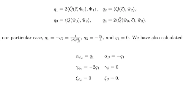
Figure 3.1: Family of equilibrium solutions shown inc−h0 space for (3.1), in collaboration with H.R. Ogrosky. A red ×represents a Hopf bifurcation.
3.1.2 Traveling Waves with Perturbation by Viscosity Consider the initial boundary value problem given by
ht+hhx+Sh3(hx+hxxx) +βhxxx = 0 inQT,
h(x,0) =h0(x),
∂xjh(a,·) =∂xjh(−a,·), for j= 0,1,2,3, t∈[0, T]
(3.9)
where Ω and QT are as before andβ >0. Integrating, we obtain a small perturbation of (3.1):
K=−cφ+1 2φ
2+Sφ3(φ0+φ000) +βφ00. (3.10)
Applying the same computations as in section 3.1.1, we consider the system given by
ψ10 =ψ2, ψ20 =ψ3,
ψ30 =fβ(ψ1, ψ2, ψ3) :=
K Sψ3
1 + c
Sψ2 1
− 1
2Sψ1
−ψ2−βψ3
ψ3 1
,
(3.11)
Bβ,J given by
Bβ,J =
0 1 0
0 0 1
J −1 − β Sφ3
H
. (3.12)
Lemma 9. Let F be given by
F(β, φe,Ψ) = (ψ2, ψ3, fβ(ψ1+φe+φH, ψ2, ψ3)) (3.13)
where Ψ = (ψ1, ψ2, ψ3). Then there exist non-trivial to
dΨ
dt −F(β, φe,Ψ) = 0 (3.14)
near the equilibrium solution Ψ = 0.
Proof. This is a specific instance of very general work in the area of degenerate Hopf bifurcations of Shearer [30]. We simply check the hypotheses of this work and note thatF satisfies the required hypotheses:
F(0,0, ~0) = 0. (H1)
ForL=Fu(0,0, ~0) and σ(L) the spectrum of L:
(i) iis an algebraically simple eigenvalue ofL (ii) 0 is an algebraically simple eigenvalue ofL (iii) ni6∈σ(L) for n= 2,3, ....
(H2)
It is clear that both of these hypotheses are met, so Shearer’s work grants the existence of traveling wave solutions to this nonlinear problem.
We now proceed by using the averaging techniques provided in [31].
Lemma 10. The problem
dΨ
has asymptotic solutions of the form
Ψ(s, ε) =ε[xΦ0(s) +y~c] +ε2w(s) +O(ε3), φe(ε) =νε,
β(ε) =εµ+O(ε2), T(ε) = 2π+O(ε2),
(3.16)
where |µ|<1, ν =±1, andw∈N(L)⊥, and
x= q
−3(µ2−1) y=µ−ν. (3.17)
Proof. In the context of [31], we have the ordinary differential equation
dΨ
dt =F(Ψ, β, φe) = [ψ2, ψ3, fβ(ψ1+φH +φe, ψ2, ψ3)], (3.18)
and infβ, we have writtencas a function of φH+φe. Note thatF satisfies the following hypotheses
F ∈C2(B), (H3)
F(β, φe, ~0) =~0 ∀(β, φe, ~0)∈B, (H4)
where B is an open ball centered at the origin inR×R×R3. It then follows that F has Taylor expansion
where
B0 = ∂F
∂Ψ(0,0, ~0) =
0 1 0
0 0 1
0 −1 0 , (3.20)
B1 = ∂2F ∂Ψ∂φe
(0,0, ~0) =− 1
Sφ3H
0 0 0 0 0 0 1 0 0 , (3.21)
B2 = ∂ 2F
∂Ψ∂β(0,0, ~0) =− 1 Sφ3 H
0 0 0 0 0 0 0 0 1 , (3.22)
Q(Ψ) = 1 2
∂2F
∂Ψ2(0,0, ~0)ΨΨ, (3.23)
is a vector of quadratic forms in Ψ, and the remainder termRsatisfies|R(β, φe,Ψ)|=o(|(β, φe,Ψ)|2).
By previous computations, it is clear that B0 satisfies the hypothesis (H2). Given that F and B0 satisfy (H2), (H3), and (H4), the matrix B(β, φe) = ∂F(β,φ∂Ψe,~0) has continuously differentiable
eigenvaluesα(β, φe)±iξ(β, φe) and γ(β, φe) satisfying α(0,0) = 0 =γ(0,0) and ξ(0,0) = 1. The
derivatives ofγ, α,and ξ can be computed to show that
αβ =
∂α
∂β(0,0)6= 0, γφe =
∂γ ∂φe
(0,0)6= 0 (H5)
holds.
We now wish to perform formal asymptotics. We first transform (3.15) into a two-point boundary value problem with periodic boundary conditions, following techniques of Langford [31]. Though we do not yet know the periodT, we expect it to be nearT0 = 2π. Sets= 2Tπtand redefine Ψ = Ψ(s) in order to obtain the system
dΨ ds =
T
2πF(β, φe,Ψ), s∈[0,2π], Ψ(0) = Ψ(2π), .
(3.24)
linearization of (3.24) at (β, φe,Ψ, T) = (0,0,0, T0) is given by dΦ
ds −B0Φ = 0, Φ(0) = Φ(2π).
(3.25)
Let~a±i~bbe the complex eigenvectors ofB0 corresponding to the eigenvalues ±iand let~cbe the real eigenvector in the nullspace of B0, all normalized so that
~a∗~a+~b∗~b= 2, ~c∗~c= 1. (3.26)
Explicitly, we have
~a= r 2 3 −1 0 1
, ~b= r 2 3 0 1 0
, ~c= 1 0 0 . (3.27)
Then (3.25) has solution space spanned by
Φ1(s) =~acoss−~bsins= Re[(~a+i~b)eit], Φ2(s) =~asins+~bcoss= Im[(~a+i~b)eit], Φ3(s) =~c.
(3.28)
Realizing that Φ2(s) = Φ1(s−π/2), we see that Φ2 gives no new information and this redundancy can be removed by methods used in [31]. Because{~a,~b, ~c}is a linearly independent set in R3, there is an~e∈R3 so that~e∗~c= 0 and~ehas non-zero projection in span{~a,~b}, say
~e= 0 0 1 . (3.29)
We now require that any solution to (3.25) satisfies
~
Define the 4×3 matricesM and N by
M = I
~e∗
, N =
−I ~0∗
, (3.31)
where I is the 3×3 identity matrix and~0∗= (0,0,0). We replace (3.24) and (3.25), respectively, dΨ
ds = T 2π
¯
F(β, φe,Ψ),
MΨ(0) +NΨ(2π) =~0,
(3.32)
and
dΦ
ds −B0Φ =~0,
MΦ(0) +NΦ(2π) =~0.
(3.33)
One sees that (3.33) has solution space spanned by~c and Φ0 given by
Φ0(s) =x1Φ1(s) +x2Φ2(s), (3.34)
where x2
1+x22= 1 and
x1~e∗~a+x2~e∗~b= 0. (3.35)
Because~e∗~b= 0,it follows thatx1 = 0 and x2 = 1, whence it follows that
Φ0(s) = r
2 3
−sin(s) cos(s) sin(s)
. (3.36)
One can further consider the adjoint problem to (3.33):
−dΨ
∗
ds −B
∗
0Ψ∗ =~0, UΨ∗(0) +VΨ∗(2π) =~0,
(3.37)