Quenched large deviation principle for words in a letter sequence

arXiv:0807.2611v2 [math.PR] 30 May 2009

Quenched large deviation principle for words in a letter sequence

Matthias Birkner 1 Andreas Greven 2 Frank den Hollander 3 4

13th May 2009

Abstract

When we cut an i.i.d. sequence of letters into words according to an independent renewal process, we obtain an i.i.d. sequence of words. In theannealed large deviation principle (LDP) for the empirical process of words, the rate function is the specific relative entropy of the observed law of words w.r.t. the reference law of words. In the present paper we consider the quenched LDP, i.e., we condition on a typical letter sequence. We focus on the case where the renewal process has analgebraic tail. The rate function turns out to be a sum of two terms, one being the annealed rate function, the other being proportional to the specific relative entropy of the observed law of letters w.r.t. the reference law of letters, with the former being obtained by concatenating the words and randomising the location of the origin. The proportionality constant equals the tail exponent of the renewal process. Earlier work by Birkner considered the case where the renewal process has an exponential tail, in which case the rate function turns out to be the first term on the set where the second term vanishes and to be infinite elsewhere. In a companion paper the annealed and the quenched LDP are applied to the collision local time of transient random walks, and the existence of an intermediate phase for a class of interacting stochastic systems is established.

Key words: Letters and words, renewal process, empirical process, annealed vs. quenched, large deviation principle, rate function, specific relative entropy.

MSC 2000: 60F10, 60G10.

Acknowledgement: This work was supported in part by DFG and NWO through the Dutch-German Bilateral Research Group “Mathematics of Random Spatial Models from Physics and Biology”. MB and AG are grateful for hospitality at EURANDOM. We also thank an anonymous referee for her/his careful reading and helpful comments.

1_{Department Biologie II, Abteilung Evolutionsbiologie, University of Munich (LMU),}

Grosshaderner Str. 2, 82152 Planegg-Martinsried, Germany

2_{Mathematisches Institut, Universit¨at Erlangen-N¨urnberg, Bismarckstrasse 1}1 2, 91054

Erlangen, Germany

3_{Mathematical Institute, Leiden University, P.O. Box 9512, 2300 RA Leiden, The}

Netherlands

1

Introduction and main results

1.1 Problem setting

Let E be a finite set of letters. Let Ee = ∪n∈NEn be the set of finite words drawn from E. Both

E and Ee are Polish spaces under the discrete topology. Let P(EN

) and P(EeN

) denote the set of probability measures on sequences drawn from E, respectively, Ee, equipped with the topology of weak convergence. Write θ and θe for the left-shift acting on EN

, respectively, EeN

. Write

Pinv_(EN

),Perg_(EN

) and Pinv_(EeN

),Perg_(EeN

) for the set of probability measures that are invariant and ergodic underθ, respectively, θe.

For ν ∈ P(E), let X= (Xi)i∈N be i.i.d. with law ν. Without loss of generality we will assume that supp(ν) =E (otherwise we replace E by supp(ν)). Forρ∈ P(N_{), letτ = (τi)i∈}N be i.i.d. with law ρhaving infinite support and satisfying the algebraic tail property

lim

n→∞

ρ(n)>0

logρ(n)

logn =:−α, α∈(1,∞). (1.1)

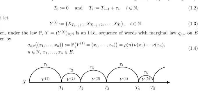
(No regularity assumption will be necessary for supp(ρ).) Assume that X and τ are independent and write P_{to denote their joint law. Cut words out ofX according toτ, i.e., put (see Figure 1)}

T0 := 0 and Ti :=Ti−1+τi, i∈N, (1.2) and let

Y(i):= XTi−1+1, XTi−1+2, . . . , XTi

, i∈N_{. (1.3)}

Then, under the law P_{, Y = (Y}(i)_)i∈N is an i.i.d. sequence of words with marginal law q_ρ,ν on Ee given by

qρ,ν (x1, . . . , xn):=P Y(1) = (x1, . . . , xn)=ρ(n)ν(x1)· · ·ν(xn),

n∈N_{, x1, . . . , xn∈E.} (1.4)

τ1

τ2 τ3

τ4

τ5

T1 T2 T3 T4 T5

Y(1) _Y(2) _Y(3) _Y(4) _Y(5)

X

Figure 1: Cutting words from a letter sequence according to a renewal process.

For N ∈ N_{, let (Y}(1)_{, . . . , Y}(N)₎per _{stand for the periodic extension of (Y}(1)_{, . . . , Y}(N)_{) to an}

element ofEeN

, and define

RN :=

1

N N_X−1

i=0

δ_θei_(Y(1)_,...,Y(N)₎per ∈ Pinv(Ee

N

), (1.5)

theempirical process of N-tuples of words. By the ergodic theorem, we have

w−lim

N→∞RN =q

⊗N

ρ,ν P–a.s., (1.6)

with w−lim denoting the weak limit. The following large deviation principle (LDP) is standard (see e.g. Dembo and Zeitouni [5], Corollaries 6.5.15 and 6.5.17). For Q∈ Pinv_(EeN

) let

H(Q|q_ρ,ν⊗N) := lim

N→∞

1

N h

Q|F_N |(q ⊗N

ρ,ν)|F_N

be thespecific relative entropy ofQw.r.t. q⊗N

ρ,ν, whereFN =σ(Y(1), . . . , Y(N)) is the sigma-algebra

generated by the first N words, Q_|F

N is the restriction of Q to

F_{N, and h(· | ·) denotes relative}

entropy. (For general properties of entropy, see Walters [13], Chapter 4.)

Theorem 1.1. [Annealed LDP] The family of probability distributions P(RN ∈ ·), N ∈ N, satisfies the LDP on Pinv_(EeN

) with rate N and with rate function Iann: Pinv_(EeN

) →[0,∞] given by

Iann(Q) =H(Q|q⊗N

ρ,ν). (1.8)

This rate function is lower semi-continuous, has compact level sets, has a unique zero atQ=q⊗N

ρ,ν, and is affine.

The LDP for RN arises from the LDP for N-tuples via a projective limit theorem. The ratio under the limit in (1.7) is the rate function forN-tuples according to Sanov’s theorem (see e.g. den Hollander [8], Section II.5), and is non-decreasing inN.

1.2 Main theorems

Our aim in the present paper is to derive the LDP for P_{(RN ∈ · |X), N ∈}N_{. To state our result,}

we need some more notation. Let κ:EeN

→EN

denote theconcatenation map that glues a sequence of words into a sequence of letters. For Q∈ Pinv_(EeN

) such that

mQ:=EQ[τ1]<∞, (1.9) define ΨQ∈ Pinv(EN) as

ΨQ(·) :=

1

mQ

E_Q "_τ1−1

X

k=0

δ_θk_κ(Y)(·)

#

. (1.10)

Think of ΨQ asthe shift-invariant version of the concatenation ofY under the law Qobtained after randomising the location of the origin.

For tr∈N_{, let [·]tr: E}e_→[Ee_{]tr :=∪}tr_n=1En _{denote the word length truncation map defined by}

y= (x1, . . . , xn)7→[y]tr:= (x1, . . . , xn∧tr), n∈N, x1, . . . , xn∈E. (1.11)

Extend this to a map from EeN

to [Ee]N tr via

(y(1), y(2), . . .)_tr := [y(1)]tr,[y(2)]tr, . . . (1.12)

and to a map from Pinv_(EeN

) to Pinv_([Ee]N tr) via [Q]tr(A) :=Q({z∈Ee

N

: [z]tr∈A}), A⊂[Ee] N

tr measurable. (1.13) Note that ifQ∈ Pinv_(EeN

), then [Q]tr is an element of the set

Pinv,fin(EeN) ={Q∈ Pinv(EeN) : mQ<∞}. (1.14)

Theorem 1.2. [Quenched LDP]Assume(1.1). Then, for ν⊗N

–a.s. allX, the family of (regular) conditional probability distributions P_{(RN ∈ · | X), N ∈} N_{, satisfies the LDP on P}inv_(EeN_{) with}

rate N and with deterministic rate function Ique: Pinv(EeN

)→[0,∞]given by

Ique(Q) :=

  

Ifin(Q), ifQ∈ Pinv,fin_(EeN ),

lim tr→∞I

fin _[Q]

tr, otherwise,

(1.15)

where

Theorem 1.3. The rate function Ique is lower semi-continuous, has compact level sets, has a unique zero atQ=q⊗N

ρ,ν, and is affine. Moreover, it is equal to the lower semi-continuous extension of Ifin _{from P}inv,fin_(EeN

) to Pinv_(EeN ).

Theorem 1.2 will be proved in Sections 3–5, Theorem 1.3 in Section 6.

A remarkable aspect of (1.16) in relation to (1.8) is that it quantifies the difference between the quenched and the annealed rate function. Note the appearance of the tail exponent α. We have not been able to find a simple formula for Ique(Q) when mQ = ∞. In Appendix A we will show

that the annealed and the quenched rate function are continuous under truncation of word lengths, i.e.,

Iann(Q) = lim tr→∞I

ann_([Q]

tr), Ique(Q) = lim tr→∞I

que_([Q]

tr), Q∈ Pinv(EeN). (1.17)

Theorem 1.2 is an extension of Birkner [2], Theorem 1. In that paper, the quenched LDP is derived under the assumption that the law ρ satisfies theexponential tail property

∃C <∞, λ >0 : ρ(n)≤Ce−λn ∀n∈N (1.18)

(which includes the case where supp(ρ) is finite). The rate function governing the LDP is given by

Ique(Q) :=

H(Q|q⊗N

ρ,ν), ifQ∈Rν,

∞, ifQ /∈R_ν, (1.19)

where

R_{ν :=}

Q∈ Pinv(EeN

) : w−lim

L→∞

1

L L_X−1

k=0

δ_θk_κ(Y) =ν⊗N Q−a.s.

. (1.20)

Think of R_{ν as the set of those Q’s for which the concatenation of words has the same statistical}

properties as the letter sequence X. This set is not closed in the weak topology: its closure is

Pinv_(EeN ).

We can include the cases whereρ satisfies (1.1) withα= 1 or α=∞.

Theorem 1.4. (a)If α= 1, then the quenched LDP holds with Ique _=Iann _{given by (1.8).} (b) If α=∞, then the quenched LDP holds with rate function

Ique(Q) =

(

H(Q|q⊗N

ρ,ν) if _tr→∞lim m[Q]trH(Ψ[Q]tr|ν

⊗N ) = 0,

∞ otherwise. (1.21)

Theorem 1.4 will be proved in Section 7. Part (a) says that the quenched and the annealed rate function are identical when α= 1. Part (b) says that (1.19) can be viewed as the limiting case of (1.16) asα→ ∞. Indeed, it was shown in Birkner [2], Lemma 2, that onPinv,fin_(EeN

):

ΨQ=ν⊗N if and only if Q∈Rν. (1.22)

Hence, (1.21) and (1.19) agree on Pinv,fin_(EeN

), and the rate function (1.21) is the lower semicon-tinuous extension of (1.19) to Pinv_(EeN

). By Birkner [2], Lemma 7, the expressions in (1.21) and (1.19) are identical if ρ has exponentially decaying tails. In this sense, Part (b) generalises the result in Birkner [2], Theorem 1, to arbitraryρ with a tail that decays faster than algebraic.

Corollary 1.5. Under the assumptions of Theorem1.2, forν⊗N

–a.s. all X, the family of (regular) conditional probability distributions P(π1RN ∈ · |X), N ∈N, satisfies the LDP on P(Ee) with rate N and with deterministic rate function I₁que: P(Ee)→[0,∞]given by

I₁que(q) := infIque(Q) : Q∈ Pinv(EeN

), π1Q=q . (1.23)

This rate function is lower semi-continuous, has compact levels sets, has a unique zero atq =qρ,ν, and is convex.

Corollary 1.5 shows that the rate function in Birkner [1], Theorem 6, must be replaced by (1.23). It does not appear possible to evaluate the infimum in (1.23) explicitly in general. For a q∈ P(Ee) with finite mean length and Ψ_q⊗N =ν⊗

N

, we have I₁que(q) =h(q|qρ,ν).

By taking projective limits, it is possible to extend Theorems 1.2–1.3 to more general letter spaces. See, e.g., Deuschel and Stroock [6], Section 4.4, or Dembo and Zeitouni [5], Section 6.5, for background on (specific) relative entropy in general spaces. The following corollary will be proved in Section 8.

Corollary 1.6. The quenched LDP also holds whenEis a Polish space, with the same rate function as in (1.15–1.16).

In the companion paper [3] the annealed and quenched LDP are applied to the collision local time of transient random walks, and the existence of an intermediate phase for a class of interacting stochastic systems is established.

1.3 Heuristic explanation of main theorems

To explain the background of Theorem 1.2, we begin by recalling a few properties of entropy. Let

H(Q) denote the specific entropy of Q∈ Pinv(EeN

) defined by

H(Q) := lim

N→∞

1

N h Q|F_N

∈[0,∞], (1.24)

where h(·) denotes entropy. The sequence under the limit in (1.24) is non-increasing in N. Since

q⊗N

ρ,ν is a product measure, we have the identity (recall (1.2–1.4))

H(Q|q⊗N

ρ,ν) =−H(Q)−EQ[logqρ,ν(Y1)] =−H(Q)−E_{Q[logρ(τ1)]−mQ}E_Ψ

Q[logν(X1)].

(1.25)

Similarly,

H(ΨQ|ν⊗

N

) =−H(ΨQ)−EΨQ[logν(X1)]. (1.26)

Below, for a discrete random variable Z with a law Q on a state space Z we will write Q(Z) for the random variable f(Z) with f(z) =Q(Z =z),z∈ Z. Abbreviate

K(N):=κ(Y(1), . . . , Y(N)) and K(∞) :=κ(Y). (1.27)

In analogy with (1.14), define

Perg,fin(EeN

) :=nQ∈ Perg(EeN

) : mQ<∞

o

Lemma 1.7. [Birkner [2], Lemmas 3 and 4]

Suppose that Q∈ Perg,fin_(EeN

) and H(Q)<∞. Then, Q-a.s.,

lim

N→∞

1

N logQ(K

(N)_{) =−m}

QH(ΨQ),

lim

N→∞

1

N logQ τ1, . . . , τN |K

(N)_=:−H

τ|K(Q),

lim

N→∞

1

N logQ Y

(1)_{, . . . , Y}(N)_=−H(Q),

(1.29)

with

mQH(ΨQ) +Hτ|K(Q) =H(Q). (1.30)

Equation (1.30), which follows from (1.29) and the identity

Q(K(N))Q(τ1, . . . , τN |K(N)) =Q(Y(1), . . . , Y(N)), (1.31)

identifiesHτ|K(Q). Think ofHτ|K(Q) as theconditional specific entropy of word lengths under the law Q given the concatenation. Combining (1.25–1.26) and (1.30), we have

H(Q|q_ρ,ν⊗N) =mQH(ΨQ|ν⊗

N

)−Hτ|K(Q)−EQ[logρ(τ1)]. (1.32)

The term−Hτ|K(Q)−EQ[logρ(τ1)] in (1.32) can be interpreted as the conditional specific relative entropy of word lengths under the law Q w.r.t. ρ⊗N

given the concatenation.

Note that mQ <∞ and H(Q) <∞ imply that H(ΨQ)<∞, as can be seen from (1.30). Also

note that −E_Ψ

Q[logν(X1)]<∞ because E is finite, and−EQ[logρ(τ1)]<∞ because of (1.1) and

mQ <∞, implying that (1.25–1.26) are proper.

We are now ready to give a heuristic explanation of Theorem 1.2. Let

RN_j1,...,jN(X), 0< j1 <· · ·< jN <∞, (1.33)

denote the empirical process of N-tuples of words when X is cut at the points j1, . . . , jN (i.e.,

when Ti = ji for i = 1, . . . , N; see (3.16–3.17) for a precise definition). Fix Q ∈ Perg,fin(EeN).

The probability P_{(RN ≈Q|X) is a sum over all N-tuples j1, . . . , jN such that R}N

j1,...,jN(X) ≈Q,

weighted byQN_i=1ρ(ji−ji−1) (withj0 = 0). The fact thatRjN1,...,jN(X)≈Qhas three consequences:

(1) The j1, . . . , jN must cut≈N substrings out ofX of total length ≈N mQ that look like the concatenation of words that are Q-typical, i.e., that look as if generated by ΨQ (possibly

with gaps in between). This means that most of the cut-points must hit atypical pieces of

X. We expect to have to shift X by ≈ exp[N mQH(ΨQ | ν⊗N)] in order to find the first

contiguous substring of length N mQ whose empirical shifts lie in a small neighbourhood of

ΨQ. By (1.1), the probability for the single increment j1−j0 to have the size of this shift is

≈exp[−N α mQH(ΨQ|ν⊗N)].

(2) The combinatorial factor exp[N H_τ|K(Q)] counts how many “local perturbations” ofj1, . . . , jN

preserve the property thatRN

j1,...,jN(X)≈Q.

The contributions from (1)–(3), together with the identity in (1.32), explain the formula in (1.16) onPerg,fin_(EeN

). Considerable work is needed to extend (1)–(3) fromPerg,fin_(EeN

) toPinv_(EeN ). This is explained in Section 3.5.

In (1), instead of having a single large increment preceding a single contiguous substring of length

N mQ, it is possible to have several large increments preceding several contiguous substrings, which

together have length N mQ. The latter gives rise to the same contribution, and so there is some

entropy associated with the choice of the large increments. Lemma 2.1 in Section 2.1 is needed to control this entropy, and shows that it is negligible.

1.4 Outline

Section 2 collects some preparatory facts that are needed for the proofs of the main theorems, including a lemma that controls the entropy associated with the locations of the large increments in the renewal process. In Section 3 and 4 we prove the large deviation upper, respectively, lower bound. The proof of the former is long (taking up about half of the paper) and requires a somewhat lengthy construction with combinatorial, functional analytic and ergodic theoretic ingredients. In particular, extending the lower bound from ergodic to non-ergodic probability measures is tech-nically involved. The proofs of Theorems 1.2–1.4 are in Sections 5–7, that of Corollary 1.6 is in Section 8. Appendix A contains a proof that the annealed and the quenched rate function are continuous under the truncation of the word length approximation.

2

Preparatory facts

Section 2.1 proves a core lemma that is needed to control the entropy of large increments in the renewal process. Section 2.2 shows that the tail property of ρ is preserved under convolutions.

2.1 A core lemma

As announced at the end of Section 1.3, we need to account for the entropy that is associated with the locations of the large increments in the renewal process. This requires the following combinatorial lemma.

Lemma 2.1. Let ω = (ωl)l∈N be i.i.d. with P(ω₁ = 1) = 1−P(ω₁ = 0) = p ∈ (0,1), and let

α∈(1,∞). For N ∈N_{, let}

SN(ω) :=

X

0<j1<···_{<jN <}∞

ωj₁=···=_ωjN=1

N

Y

i=1

(ji−ji−1)−α (j0 = 0) (2.1)

and put

lim sup

N→∞

1

N logSN(ω) =:−φ(α, p) ω−a.s. (2.2)

(the limit being ω-a.s. constant by tail triviality). Then

lim

p↓0

φ(α, p)

αlog(1/p) = 1. (2.3)

Proof. Let τN := min{l ∈ N: ωl = ωl+1 = · · · = ωl+N−1}. In (2.1), choosing j1 = τN and ji=ji−1+ 1 for i= 2, . . . , N, we see thatSN(ω)≥τ_N−α. Since

lim

N→∞

1

we have

φ(α, p)≤αlog(1/p) ∀p∈(0,1). (2.5)

To show that this bound is sharp in the limit asp↓0, we estimate fractional moments of SN(ω).

For any β∈(1/α,1], using that (u+v)β ≤uβ+vβ,u, v ≥0, we get

Eh_SN(ω)βi_≤ X

0<j1<···<jN<∞

Eh1

{ωj1=···=ωjN=1}

N

Y

i=1

(ji−ji−1)−αβ

i

= X

0<j1<···<jN<∞

pN N

Y

i=1

(ji−ji−1)−αβ

=p ζ(αβ)N,

(2.6)

whereζ(s) =P_n∈Nn−s,s >1, is Riemann’sζ-function. Hence, for anyε >0, Markov’s inequality yields

P ₁

N logSN(ω)≥

1

β

logp+ logζ(αβ) +ε

=P_SN(ω)β _≥eεN_{p ζ(αβ)}N_≤e−εN_{p ζ(αβ)}−NEh_SN(ω)βi_≤e−εN_.

(2.7)

Thus, by the first Borel-Cantelli Lemma,

−φ(α, p) = lim sup

N→∞

1

N logSN(ω)≤

1

β

logp+ logζ(αβ) a.s. (2.8)

Now let p↓0, followed byβ ↓1/αto obtain the claim.

Remark 2.2. Note that E_{[SN(ω)] = (pζ(α))}N_{, while typically SN(ω) ≈ p}αN_{. In the above}

computation, this is verified by bounding suitable non-integer moments ofSN(ω)/pαN. Estimating

non-integer moments in situations when the mean is inconclusive is a useful technique in a variety of different probabilistic contexts. See, e.g., Holley and Liggett [9] and Toninelli [12]. The proof of Lemma 2.1 above is similar to that of Toninelli [12], Theorem 2.1.

2.2 Convolution preserves polynomial tail

The following lemma will be needed in Sections 3.3 and 3.5. For m∈N_{, letρ}∗m _{denote them-fold}

convolution ofρ.

Lemma 2.3. Suppose thatρ satisfies ρ(n)≤Cρn−α, n∈N, for someCρ<∞. Then

ρ∗m(n)≤(Cρ∨1)mα+1n−α ∀m, n∈N. (2.9)

Proof. If n≤m, then the right-hand side of (2.9) is ≥1. So, let us assume that n > m. Then

ρ∗m(n) = X

x₁,...,xm≥1

x₁₊···+xm=n

m

Y

i=1

ρ(xi)≤ m

X

j=1

X

x1,...,xm≥1

x1+···+xm=n

xj=x1∨···∨xm

ρ(xj) m

Y

i6=j ρ(xi)

≤m Cρ⌈n/m⌉−α

X

x1,...,xm−1≥1

m_Y−1

i=1

ρ(xi)

=m Cρ⌈n/m⌉−α ≤Cρmα+1n−α.

3

Upper bound

The following upper bound will be used in Section 5 to derive the upper bound in the definition of the LDP.

Proposition 3.1. For any Q ∈ Pinv,fin(EeN

) and any ε > 0, there is an open neighbourhood

O(Q)⊂ Pinv_(EeN

) of Q such that

lim sup

N→∞

1

N logP RN ∈ O(Q)|X

≤ −Ifin(Q) +ε X−a.s. (3.1)

We remark that since |E|<∞ we automatically haveIfin(Q)∈[0,∞) for all Q∈ Pinv,fin_(EeN ), so the right-hand side of (3.1) is finite.

Proof. It suffices to consider the case ΨQ6=ν⊗N. The case ΨQ =ν⊗N, for whichIfin(Q) =H(Q| q⊗N

ρ,ν) as is seen from (1.16), is contained in the upper bound in Birkner [2], Lemma 8. Alternatively,

by lower semicontinuity ofQ′ _7→H(Q′ _|q⊗N

ρ,ν), there is a neighbourhoodO(Q) such that

inf

Q′_∈O(Q)H(Q ′_|q⊗N

ρ,ν)≥H(Q|q⊗

N

ρ,ν)−ε=Ifin(Q)−ε, (3.2)

where O(Q) denotes the closure of O(Q) (in the weak topology), and we can use the annealed bound.

In Sections 3.1–3.5 we first prove Proposition 3.1 under the assumption that there exist α ∈

(1,∞), Cρ<∞ such that

ρ(n)≤Cρn−α, n∈N, (3.3)

which is needed in Lemma 2.3. In Section 3.6 we show that this can be replaced by (1.1). In Sections 3.1–3.4, we first consider Q ∈ Perg,fin_(EeN

) (recall (1.28)). Here, we turn the heuristics from Section 1.3 into a rigorous proof. In Section 3.5 we remove the ergodicity restriction. The proof is long and technical (taking up more than half of the paper).

3.1 Step 1: Consequences of ergodicity

We will use the ergodic theorem to construct specific neighborhoods of Q∈ Perg,fin_(EeN

) that are well adapted to formalize the strategy of proof outlined in our heuristic explanation of the main theorem in Section 1.3.

Fix ε1, δ1 >0. By the ergodicity ofQ and Lemma 1.7, the event (recall (1.9) and (1.27))

1

M|K

(M)_{| ∈mQ+ [−ε} 1, ε1]

∩

− 1

M logQ(K

(M)_)∈m

QH(ΨQ) + [−ε1, ε1]

∩

− 1

M logQ(Y

(1)_{, . . . , Y}(M)_{)∈H(Q) + [−ε} 1, ε1]

∩

  

1

M

|K(M)_| X

k=1

logν((K(M))k)∈mQEΨQ

logν(X1)+ [−ε1, ε1]

  

∩

(

1

M M

X

i=1

logρ(τi)∈EQlogρ(τ1)+ [−ε1, ε1]

)

has Q-probability at least 1−δ1/4 for M large enough (depending on Q), where |K(M)| is the length of the string of letters K(M)_{. Hence, there is a finite number A of sentences of length M,} denoted by

(za)a=1,...,A withza:= (y(a,1), . . . , y(a,M))∈EeM, (3.5)

such that fora= 1, . . . , A,

|κ(za)| ∈

h

M(mQ−ε1), M(mQ+ε1)

i

,

Q(K(M)=κ(za))∈

h

exp[−M(mQH(ΨQ) +ε1)],exp[−M(mQH(ΨQ)−ε1)]

i

,

Q (Y(1), . . . , Y(M)) =za∈

h

exp[−M(H(Q) +ε1)],exp[−M(H(Q)−ε1)]

i

,

|κ_X(za)|

k=1

logν((κ(za))k)∈

h

M(mQEΨQ[logν(X1)]−ε1), M(mQEΨQ[logν(X1)] +ε1)

i

,

M

X

i=1

logρ(|y(a,i)|)∈hM(E_{Q[logρ(τ1)]−ε1), M(}E_{Q[logρ(τ1)] +ε1)}i_,

(3.6)

and

A

X

a=1

Q(Y(1), . . . , Y(M)) =za

≥1−δ1

2. (3.7)

Note that (3.7) and the third line of (3.6) imply that

A∈h 1−δ1

2

expM(H(Q)−ε1),expM(H(Q) +ε1)i. (3.8)

Abbreviate

A _{:={za, a= 1, . . . , A}. (3.9)}

Let

B_:=ζ(b)_{, b= 1, . . . , B =κ(za), a= 1, . . . , A (3.10)}

be the set of strings of letters arising from concatenations of the individual za’s, and let

Ib :=

1≤a≤A: κ(za) =ζ(b) , b= 1, . . . , B, (3.11)

so that |Ib|is the number of sentences inA giving a particular string inB. By the second line of

(3.6), we can boundB as

B ≤expM(mQH(ΨQ) +ε1), (3.12) because PB_b=1Q(K(M) = ζ(b)) ≤ 1 and each summand is at least exp[−M(mQH(ΨQ) +ε1)]. Furthermore, we have

|Ib| ≤expM(Hτ|K(Q) + 2ε1), b= 1, . . . , B, (3.13)

since

exp−M(mQH(ΨQ)−ε1)≥Q κ(Y(1), . . . , Y(M)) =ζ(b)

≥X

a∈Ib

Q (Y(1), . . . , Y(M)) =za≥ |Ib|exp−M(H(Q) +ε1),

3.2 Step 2: Good sentences in open neighbourhoods

Define the following open neighbourhood ofQ(recall (3.9))

O:=nQ′∈ Pinv(EeN ) : Q′_|F

M(

A_)>1−δ1o_{. (3.15)}

Here, Q(z) is shorthand for Q((Y(1)_{, . . . , Y}(M)_{) = z). For x ∈ E}N

and for a vector of cut-points (j1, . . . , jN)∈NN with 0< j1 <· · ·< jN <∞and N > M, let

ξN := (ξ(i))i=1,...,N = x|(0,j1], x|(j1,j2], . . . , x|(jN−1,jN]

∈EeN (3.16)

(with (0, j1] shorthand notation for (0, j1]∩N, etc.) be the sequence of words obtained by cutting

x at the positionsji, and let

RN_j1,...,jN(x) := 1

N N_X−1

i=0

δ_e

θi(ξN)per (3.17)

be the corresponding empirical process. By (3.15),

R_jN_1,...,jN(x)∈ O =⇒

#n1≤i≤N−M: x|(ji−1,ji], . . . , x|(ji+M−1,ji+M]

∈Ao_{≥N(1−δ1)−M.}

(3.18)

Note that (3.18) implies that the sentence ξN contains at least

C :=⌊(1−δ1)N/M⌋ −1 (3.19)

disjoint subsentences from the set A_{, i.e., there are 1 ≤i1, . . . , iC ≤ N −M with ic−ic−1 ≥M}

forc= 1, . . . , C such that

ξ(ic)_{, ξ}(ic+1)_{, . . . , ξ}(ic+M−1)_{∈A (3.20)}

(we implicitly assume thatN is large enough so thatC >1). Indeed, we can e.g. construct theic’s

iteratively as

i0 =−M,

ic = min

n

k≥ic−1+M: a sentence fromA starts at positionkinξN

o

,

c= 1, . . . , C,

(3.21)

and we can continue the iteration as long as cM +δ1N ≤N. But (3.20) in turn implies that the

jic’s cut out ofx at leastC disjoint subwords fromB, i.e.,

x|(jic,jic+M]∈B, c= 1, . . . , C. (3.22)

3.3 Step 3: Estimate of the large deviation probability

Using Steps 1 and 2, we estimate (recall (3.15))

P _{RN ∈ O |X=} X

0<j1<···<jN<∞

1O R N

j1,...,jN(X)

YN

i=1

ρ(ji−ji−1) (3.23)

filling subsentences

good subsentences medium ≈ΨQ X

Figure 2: Looking for good subsentences and filling subsentences (see below (3.25)).

into a sentence ofN words. By (3.22), at least C (recall 3.19) of the jc’s must be cut-points where a word fromB _{is written onX, and theseC subwords must be disjoint. As words in}B _{arise from}

concatenations of sentences from A_{, this means we can find}

ℓ1 <· · ·< ℓC, {ℓ1, . . . , ℓC} ⊂ {0, j1, . . . , jN} and ζ1, . . . , ζC ∈A (3.24)

such that

X|(ℓc,ℓc+|κ(ζc)|]=κ(ζc) =:η

(c) _{∈B and ℓ}

c ≥ℓc−1+|κ(ζc−1)|, c= 1, . . . , C−1. (3.25)

We callζ1, . . . , ζC thegood subsentences.

Note that once we fix the ℓc’s and the ζc’s, this determines C+ 1filling subsentences (some of

which may be empty) consisting of the words between the good subsentences. See Figure 2 for an illustration. In particular, this determines numbersm1, . . . , mC+1 ∈Nsuch thatm1+· · ·+mC+1=

N −CM, where mc is the number of words we cut between the (c −1)-st and the c-th good subsentence (and mC+1 is the number of words after theC-th good subsentence).

Next, let us fix good ℓ1<· · ·< ℓC and η(1), . . . , η(C)∈B, satisfying

X|_{(ℓc,ℓc+|η}(c)_|]=η(c), ℓc ≥ℓc−1+|η(c−1)|, c= 1, . . . , C. (3.26)

To estimate how many different choices of (j1, . . . , jN) may lead to this particular ((ℓc),(η(c))), we

proceed as follows. There are at most

2M ε1C expM Hτ|K(Q) + 2ε1C ≤expN Hτ|K(Q) +δ2 (3.27)

possible choices for the word lengths inside these good subsentences. Indeed, by the first line of (3.6), at most 2M ε1 different elements ofB can start at any given positionℓc and, by (3.13), each

of them can be cut in at most expM(Hτ|K(Q) + 2ε1)

different ways to obtain an element of A_.

In (3.27), δ2 = δ2(ε1, δ1, M) can be made arbitrarily small by choosing M large and ε1, δ1 small. Furthermore, there are at most

N −C(M −1)

C

≤exp[δ3N] (3.28)

Next, we estimate the value of QN_i=1ρ(ji −ji−1) for any (j1, . . . , jN) leading to the given

((ℓc),(η(c))). In view of the fifth line of (3.6), we have N

Y

i=1

ρ(ji−ji−1)

1{the

i-th word falls inside theC good subsentences}

≤expCM E_{Q[logρ(τ1)] +ε1}

≤expN E_{Q[logρ(τ1)] +δ4,}

(3.29)

where δ4 =δ4(ε1, δ1, M) can be made arbitrarily small by choosing M large andε1, δ1 small. The filling subsentences have to exactly fill up the gaps between the good subsentences and so, for a given choice of (ℓc), (η(c)) and (mc), the contribution to QNi=1ρ(ji−ji−1) from the filling subsentences is

QC

c=1ρ∗mc(ℓc−ℓc−1− |η(c−1)|) (the term forc= 1 is to be interpreted as ρ∗m1(ℓ1), andρ∗0 asδ0). By Lemma 2.3, using (3.3),

C

Y

c=1

ρ∗mc _ℓ

c−ℓc−1− |η(c−1)|

≤(Cρ∨1)C C

Y

c=1

mα_c+1

! _C Y

c=1

(ℓc−ℓc−1− |η(c−1)|)∨1−α

≤(Cρ∨1)CN −CM

C

(α+1)CYC

c=1

(ℓc−ℓc−1− |η(c−1)|)∨1−α

≤exp[N δ5]

C

Y

c=1

(ℓc−ℓc−1− |η(c−1)|)∨1−α,

(3.30)

where δ5 = δ(δ1, M) can be made arbitrarily small by choosing M large and δ1 small. For the second inequality, we have used the fact that the product QC_c=1mα_c+1 is maximal when all factors are equal.

Combining (3.23–3.30), we obtain

P _{RN ∈ O |X≤exp}h_{NHτ|K(Q) +}E_{Q[logρ(τ1)] +δ2+δ3+δ4+δ5}i

× X

(ℓc), (η(c)) good

C

Y

c=1

(ℓc−ℓc−1− |η(c−1)|)∨1−α.

(3.31)

Combining (3.31) with Lemma 3.2 below, and recalling the identity in (1.32), we obtain the result in Proposition 3.1 for ρ satisfying (3.3), with O defined in (3.15) and ε= δ2+δ3+δ4+δ5+δ6. Note thatεcan be made arbitrarily small by choosing ε1, δ1 small andM large.

3.4 Step 4: Cost of finding good sentences

Lemma 3.2. For ε1, δ1 >0 and M ∈N,

lim sup

N→∞

1

N log

 

 X

(ℓc),(η

(c)_{) good}

C

Y

c=1

(ℓc−ℓc−1− |η(c−1)|)∨1−α

  

≤ −α mQH(ΨQ|ν⊗N) +δ6 a.s.,

(3.32)

Proof. Note that, by the fourth line of (3.6), for any η∈B _{(recall (3.10)) and k∈}N_,

P _{ηstarts at positionkinX≤expM mQ}E_Ψ

Q[logν(X1)] +ε1

. (3.33)

Combining this with (3.12), we get

P _{some element of}B _{starts at positionkinX}

≤expM mQEΨQ[logν(X1)] +ε1

×expM mQH(ΨQ) +ε1

= exp−M mQH(ΨQ|ν⊗

N

)−2ε1,

(3.34)

where we use (1.26).

Next, we coarse-grain the sequenceX into blocks of length

L:=⌊M(mQ−ε1)⌋, (3.35)

and compare the coarse-grained sequence with alow-density Bernoulli sequence. To this end, define a {0,1}-valued sequence (Al)l∈N inductively as follows. Put A₀ := 0, and, for l ∈ N given that

A0, A1, . . . , Al−1 have been assigned values, define Al by distinguishing the following two cases:

(1) IfAl−1 = 0, then

Al:=

  

1, if inX there is a word η∈B_{starting in ((l−1)L, lL],}

0, otherwise.

(3.36)

(2) IfAl−1 = 1, then

Al:=

      

1, if inX there are words η, η

′ _{∈B starting in ((l−2)L,(l−1)L],} respectively, ((l−1)L, lL] and occurring disjointly,

0, otherwise.

(3.37)

Put

p:=L exp−M mQH(ΨQ|ν⊗

N

)−2ε1. (3.38)

Then we claim

P_{(A1=a1, . . . , An=an)≤p}a1+···+an_{, n∈N, a}

1, . . . , an∈ {0,1}. (3.39) In order to verify (3.39), fix a1, . . . , an ∈ {0,1} with a1+· · ·+an =m. By construction, for the

event in the left-hand side of (3.39) to occur there must be m non-overlapping elements of B _at

certain positions inX. By (3.34), the occurrence of any mfixed starting positions has probability at most

exp−mM mQH(ΨQ |ν⊗

N )−2ε1

, (3.40)

while the choice of the al’s dictates that there are at most Lm possibilities for the starting points

of the m words.

By (3.39), we can couple the sequence (Al)l∈N with an i.i.d. Bernoulli(p)-sequence (ω_l)_l∈N such that

Al≤ωl ∀l∈N a.s. (3.41)

coordinates is dense in the set of continuous increasing functions on{0,1}N

, and use the results in Strassen [11].)

Each admissible choice of ℓ1, . . . , ℓC in (3.32) leads to a C-tuple i1 < · · · < iC such that Ai1 = · · · = AiC = 1 (since it cuts out non-overlapping words, which is compatible with (3.36–

3.37)), and for any such (i1, . . . , iC) there are at most LC different admissible choices of the ℓc’s.

Thus, we have

X

(ℓc), (η(c)) good

C

Y

c=1

(ℓc−ℓc−1− |η(c−1)|)∨1−α≤LCL−α

X

0<i₁<···_{<iC <}∞

Ai₁=···=_Ai

C=1

C

Y

c=1

(ic−ic−1)−α. (3.42)

Using (3.19) and recalling the definition of φ(α, p) in (2.2), we have

lim sup

N→∞

1

N log [ r.h.s. (3.42) ]≤

1−δ1

M

log M mQ

−φ(α, p) (ω, A)−a.s. (3.43)

From (3.38) we know that log(1/p) ∼M(mQH(ΨQ|ν⊗N)−2ε1) asM → ∞and so, by Lemma 2.1, we have

r.h.s. (3.43)≤ −(1−ε2)α mQH(ΨQ |ν⊗N)−2ε1 (3.44) for anyε2 ∈(0,1), providedM is large enough. This completes the proof of Lemma 3.2, and hence of Proposition 3.1 forQ∈ Perg,fin_(EeN

).

3.5 Step 5: Removing the assumption of ergodicity

Sections 3.1–3.4 contain the main ideas behind the proof of Proposition 3.1. In the present section we extend the bound from Perg,fin_(EeN

) to Pinv,fin_(EeN

). This requires setting up a variant of the argument in Sections 3.1–3.4 in which the ergodic components of Q are “approximated with a common length scale on the letter level”. This turns out to be technically involved and to fall apart into 6 substeps.

Let Q∈ Pinv,fin(EeN

) have a non-trivial ergodic decomposition

Q=

Z

Perg₍EeN₎

Q′WQ(dQ′), (3.45)

where WQ is a probability measure on Perg(EeN) (Georgii [7], Proposition 7.22). We may assume

w.l.o.g. that H(Q|q⊗N

ρ,ν)<∞, otherwise we can simply employ the annealed bound. Thus,WQ is

in fact supported onPerg,fin(EeN

)∩ {Q′: H(Q′|q⊗N

ρ,ν)<∞}.

Fixε >0. In the following steps, we will construct an open neighbourhoodO(Q)⊂ Pinv(EeN ) of

Qsatisfying (3.1) (for technical reasons withεreplaced by someε′_=ε′_{(ε) that becomes arbitrarily} small as ε↓0).

3.5.1 Preliminaries

Observing that

mQ =

Z

Perg₍EeN₎

mQ′W_Q(dQ′)<∞, H(Q|q⊗_ρ,νN) =

Z

Perg₍EeN₎

H(Q′|q_ρ,ν⊗N)WQ(dQ′)<∞, (3.46)

we can findK0, K1, m∗>0 and a compact set

C _{⊂ P}inv_(EeN_{)∩supp(WQ)∩ {Q: H(·|q}⊗N

such that

sup{H(ΨP |ν⊗N) : P ∈C} ≤K1, (3.48)

sup{mP: P ∈C} ≤m∗, (3.49)

the family{L_{P(τ1) : P ∈}C_{}is uniformly integrable, (3.50)}

WQ(C_{)≥1−ε/2, (3.51)}

Z

C

H(Q′|q⊗_ρ,νN)WQ(dQ′)≥H(Q|q⊗

N

ρ,ν)−ε/2, (3.52)

Z

C

mQ′H(Ψ_Q′|ν⊗N)W_Q(dQ′)≥m_QH(Ψ_Q|ν⊗N)−ε/2. (3.53)

In order to check (3.50), observe that E_{Q[τ1] < ∞ implies that there is a sequence (cn) with}

limn→∞cn=∞such that

E_Qτ11{τ

1≥cn}

≤ 6

π2_n3

ε

6, n∈N. (3.54)

Put

b

An:={Q′ ∈ Pinv(EeN) : EQ′τ₁1{τ

1≥cn}

>1/n} (3.55)

and A:=∩n∈N(Anb )c. EachAnb is open, henceA is closed, and by the Markov inequality we have

WQQ′: EQ′τ₁1

{τ1≥cn}

>1/n ≤nE_Qτ11

{τ1≥cn}

≤ 6

π2_n2

ε

6. (3.56)

Thus,

WQ(Ac) =WQ ∪n∈NAb_n

≤ ε

6

X

n∈N 6

π2_n2 =

ε

6. (3.57)

This implies that the mapping

Q′ 7→mQ′H(Ψ_Q′|ν⊗N) is lower semicontinuous on C. (3.58) Indeed, if w−limn→∞Q′n = Q′′ and (Q′n) ⊂ C, then limn→∞EQ′

n[τ1] = limn→∞mQ′n = mQ′′ =

E_Q′′[τ₁] and w−lim_n→∞Ψ_Q′

n = ΨQ′′ by uniform integrability (see Birkner [2], Remark 7).

Furthermore, we can find N0, L0 ∈ N with L0 ≤N0 and a finite set Wf ⊂ EeN0 such that the following holds. Let

W :=nπL0(θ

i_{κ(ζ)) : ζ = (ζ}(1)_{, . . . , ζ}(N0)_)∈f_{W ,0≤i <|ζ}(1)_|o _(3.59)

be the set of words of lengthL0 obtained by concatenating sentences from fW, possibly shifting the “origin” inside the first word and restricting to the firstL0 letters. Then, denoting byD the set of all P ∈ Pinv,fin_(EeN

)∩C _{that satisfy}

X

ζ∈fW

P(ζ)≥1− ε

3c_⌈3/ε⌉, ∀ξ∈W : ΨP(ξ)≤

1 +ε/2

mP

E_Ph1f

W(πN0Y)

τ_X1−1

i=0

1

{ξ}(πL0θ

i_κ(Y))i _(3.60)

H(P |q_ρ,ν⊗N) +ε/4≥ 1

N0

X

ζ∈fW

P(ζ) log P(ζ)

q⊗N0

ρ,ν (ζ)

≥H(P |q_ρ,ν⊗N)−ε/4, (3.61)

mPH(ΨP |ν⊗

N

) +ε/4≥ mP

L0

X

w∈W

ΨP(w) log

ΨP(w)

ν⊗L0_(w) ≥mPH(ΨP |ν

⊗N

we can choose N0,L0 and fW so large that the following inequalities hold:

WQ(D) ≥ 1−3ε/4, (3.63)

Z

D

H(P |q⊗N

ρ,ν)WQ(dP) ≥ H(Q|qρ,ν⊗N)−3ε/4, (3.64)

Z

D

mPH(ΨP|ν⊗N)WQ(dP) ≥ mQH(ΨQ |ν⊗N)−3ε/4. (3.65)

We may choose the setWf in such a way that

δ_fW := min{q⊗N0

ρ,ν (ζ) :ζ ∈Wf} ·

min{ν⊗L0_{(ξ) : ξ ∈W}}

max{|ζ(1)_{|: ζ ∈Wf}} · 1

|fW|>0. (3.66)

3.5.2 Approximating with a given length scale on the letter level

ForP ∈ Pinv,fin_(EeN

), we put

δ_P,fW :=δ_fW ·minP(ζ) : ζ ∈W , Pf (ζ)>0 ∧minΨP(ξ) : ξ∈W,ΨP(ξ)>0 . (3.67)

Forδ >0 andL∈N_{, we say thatP ∈ P}inv,fin_(EeN

) can be (δ, L)-approximatedif there exists a finite subsetA_{P ⊂E}e⌈L/mP⌉ _{of “P-typical” sentences, each consisting of ≈L/mP words (we assume that}

L > N0mP), such that

P_|F

⌈_L/mP⌉(

A_P)>1−1

2δ·δP,Wf (3.68)

and, for allz= (y(1), . . . , y(⌈L/mP⌉)_)∈A_P,

P(z)∈hexp− ⌈L/mP⌉(H(Q) +δ),exp− ⌈L/mP⌉(H(Q)−δ)i,

|κ(z)| ∈[L(1−δ), L(1 +δ)],

P K(⌈L/mP⌉) _=z∈h_exp−L(H(Ψ

Q) +δ),exp[−L(H(ΨQ)−δ)i,

|κ(z)|

X

k=1

logν(κ(z)k)∈[L(1−δ), L(1 +δ)]EΨP

logν(X1),

⌈L/m_XP⌉

i=1

logρ(|y(i)|)∈[(L/mP)(1−δ),(L/mP)(1 +δ)]EPlogρ(τ1),

|{z′ ∈A_{P: κ(z) =κ(z}′_{)}| ≤exp(L/mP)(Hτ|K(P) +δ).}

(3.69)

By the third and the fourth line of (3.69) we have, using (1.26),

P _{Xstarts with some element ofκ(}A_P)≤exph_{−L(1−2δ)H ΨQ |ν}⊗Ni_{. (3.70)}

ForP that can be (δ, L)-approximated, define an open neighbourhood ofP via

U(δ,L)(P) :=

P′ ∈ Pinv(EeN) : P ′_(z)

P(z) ∈(1−δ·δP,Wf,1 +δ·δP,fW) ∀z∈AP

, (3.71)

where A_{P =}A_{P(δ, L) is the set from (3.68–3.69). By the results of Section 3.1 and the above, for}

given P ∈ Perg,fin_(EeN

)∩C _{and δ0 >0 there existδ}′ _{∈(0, δ0) andL}′ _{such that}

Assume that a given P ∈D _{can be (δ, L)-approximated for some L such that ⌈L/mP⌉ ≥N0.}

We claim that then for any P′ _{∈D∩ U}

(δ,L)(P),

P′(Ee⌈L/mP⌉_\A

P)≤ 2δ·δ_P,fW, (3.73)

∀ζ∈Wf: P′(ζ)≤

(

(1 + 3δ)P(ζ) ifP(ζ)>0,

2δ·δ_P,fW (≤2δ·min{q⊗N0

ρ,ν (ζ′) : ζ′ ∈Wf}) otherwise,

(3.74)

∀ξ ∈W: mP′Ψ_P′(ξ)≤

(

(1 +ε/2)(1 + 3δ)mPΨP(ξ) if ΨP(ξ)>0,

(1 +ε/2)2δmin{ν⊗L0_(ξ′_{) : ξ}′_{∈W} otherwise,} (3.75)

mP′ ≥(1−3δ)(m_P −ε) (≥(1−3δ−ε)m_P). (3.76)

(3.73) follows from (3.68) and (3.71). To verify (3.74), note that, forζ ∈fW,

P′(ζ)≤ X

z∈A_P: πN0(z)=ζ

P′(z) + X

z∈Ee⌈_L/mP⌉_\A_{P: πN} 0(z)=ζ

P′(z)

≤(1 +δ) X

z∈A_P:πN 0(z)=ζ

P(z) +P′ Ee⌈L/mP⌉_\A

P

(3.77)

and use (3.73) on the last term in the second line, observing that δ_P,Wf ≤ P(ζ) whenever ζ ∈Wf

and P(ζ)>0. To verify (3.75), observe that, for ξ ∈W (recall the definition of ΨP′ from (1.10)), using (3.60),

(1 +ε/2)−1mP′Ψ_P′(ξ)≤

X

ζ∈Wf P′(ζ)

|ζ(1)_|−1 X

i=0

1{ξ} πL

0(θ

i_κ(ζ))

≤(1 +δ)mPΨP(ξ) +

X

ζ∈fW: P(ζ)=0

|ζ(1)|P′(ζ)

(3.78)

and that the sum in the second line above is bounded by |Wf| ·max{|ζ(1)_{| : ζ ∈ fW} ·2δ ·δ}

P,Wf,

which is not more than 2δmPΨP(ξ) if ΨP(ξ) > 0 and not more than 2δmin{ν⊗L0(ξ′) : ξ′ ∈ W}

otherwise. Lastly, to verify (3.76), note that

P′(ζ)≥(1−3δ)P(ζ) ∀ζ ∈Wf (3.79)

(which can be proved in the same way as (3.74)), so that

mP′ =

X

y∈Ee

|y|P′(y)≥ X

ζ∈Wf

|ζ(1)|P′(ζ)≥(1−3δ) X

ζ∈Wf

|ζ(1)|P(ζ). (3.80)

Furthermore,

mP ≤

X

ζ∈Wf

|ζ(1)|P(ζ) +c_⌈3/ε⌉P EeN0_\Wf₊ X

y∈Ee: |y|>c⌈3/ε⌉

|y|P(y). (3.81)

Observing that the second and the third term on the right-hand side are each at mostε/3, we find that (3.80–3.81) imply (3.76).

Finally, observe that (3.74–3.76) imply that there exists δ0(= δ0(ε)) > 0 with the following property: For anyP, P′ ∈D_{such thatP can be (δ, L)-approximated for someLwith⌈L/mP⌉ ≥N0}

and δ≤δ0 and P′ ∈ U(δ,L)(P), we have

H(P′ |q⊗_ρ,νN) ≤ (1 +ε)H(P |q⊗_ρ,νN) +ε and (3.82)

mP′H(Ψ_P′ |ν⊗N) ≤ (1 +ε)

mPH(ΨP |ν⊗N) +ε

Here, (3.82) follows from the observation

H(P′ |q⊗_ρ,νN)−ε

4

≤ 1

N0

X

ζ∈fW

P′(ζ) log P ′_(ζ)

q⊗N0

ρ,ν (ζ)

≤ 1 + 3δ

N0

X

ζ∈fW

P(ζ) log(1 + 3δ)P(ζ)

q⊗N0

ρ,ν (ζ)

+ 1

N0

X

ζ∈fW:P(ζ)=0

P′(ζ) logmin{q ⊗N0

ρ,ν (ζ′) :ζ′∈fW} q⊗N0

ρ,ν (ζ)

≤(1 + 3δ)H(P |q⊗N

ρ,ν) + ε

4

+ 1 + 3δ

N0

log(1 + 3δ).

(3.84)

Similarly, observing that

mP′

X

ξ∈W

ΨP′(ξ) log mP

′Ψ_P′(ξ)

mP′ν⊗L0(ξ)

≤1 +ε 2

(1 + 3δ)mP

X

ξ∈W

ΨP(ξ) log

(1 +ε/2)(1 + 3δ)mPΨP(ξ)

(1−3δ−ε)mPν⊗L0(ξ)

+mP′

X

ξ∈W: ΨP(ξ)=0

ΨP′(ξ) log(1 +ε/2)2δmin{ν

⊗L0_(ξ′_{) : ξ}′_∈W}

ν⊗L0(ξ)

≤1 +ε 2

(1 + 3δ)L0mPH(ΨP |ν⊗N) +ε/2 +m∗log(1 + 3δ)(1 +ε/2)

1−3δ−ε

(3.85)

we obtain (3.83) in view of (3.62).

3.5.3 Approximating the ergodic decomposition

In the previous subsection, we have approximated a givenP ∈ Perg,fin_(EeN

), i.e., we have constructed a certain neighbourhood of P w.r.t. the weak topology, which requires only conditions on the frequencies of sentences whose concatenations are ≈ L letters long. While the required L will in general vary with P, we now want to construct a compact C′ _⊂C _{such that WQ(}C′_{) is still close}

to 1 and allP ∈C′ _{can be approximated on the same scaleL (on the letter level). To this end, let} D_ε′_,L′ :=P ∈D: P can be (ε′, L′)-approximated . (3.86) By (3.72), we have

[

ε′∈(0,ε/2)

L′∈N

D_ε′_,L′ =Perg,fin(EeN)∩C, (3.87)

so, in view of (3.51–3.53), we can choose

0< ε1<

ε

2m∗_(1∨K1) ∧

δ0

2 (3.88)

and L∈N_{such that}

WQ(Dε1,L) ≥ 1−ε, (3.89) Z

D_ε 1,L

H(Q′ |q_ρ,ν⊗N)WQ(dQ′) ≥ H(Q|q⊗

N

ρ,ν)−ε, (3.90)

Z

D_ε 1,L

ForP ∈D_ε

1,L, let

U′(P) :=

P′ ∈ Pinv(EeN) : P ′_(z)

P(z) ∈

1−ε1

2 δP,Wf,1 + ε1

2δP,Wf

∀z∈A_P

, (3.92)

where A_{P is the set from (3.68–3.69) that appears in the definition of U(ε}

1,L)(P) and δP,fW is

defined in (3.67). Note that U′(P) ⊂ U(ε1,L)(P). Indeed, infP∈Dε1,Ldist(U

′_(P),U

(ε1,L)(P)

c_{) >0 if}

we metrize the weak topology. Consequently,

C′ _:=C _{∩ ∪P∈D}

ε1,LU′(P) ⊃Dε1,L

(3.93)

is compact and satisfies WQ(C′)≥1−ε, and

C′_⊂ [

P∈D_ε 1,L

U(ε1,L)(P) (3.94)

is an open cover. By compactness there exist R ∈ N _{and (pairwise different) Q1, . . . , QR ∈}

Perg,fin_(EeN

)∩C _{such that}

U(ε1,L)(Q1)∪ · · · ∪ U(ε1,L)(QR)⊃C

′_{, (3.95)}

whereU(ε1,L)(Qr) is of the type (3.71) with a set Ar⊂Ee

Mr _{satisfying (3.68–3.69) withP replaced}

by Qr, and Mr =⌈L/mQr⌉.

For z ∈ ∪n∈NEen consider the probability measure on [0,1] given by µ_Q,z(B) := W_Q({Q′ ∈

Perg,fin_(EeN

) : Q′(z)∈B}), B ⊂[0,1] measurable. Observing that

R

[

r=1

[

z∈A_r

u∈[0,1] : u is an atom of µQ,z (3.96)

is at most countable, we can findε2 ∈[ε1, ε1+ε12) (note that still ε2 <2ε1) and eδ >0 such that

WQ

  

    Q

′ _{∈ P}erg,fin_(EeN ) :

Q′(z)/Qr(z)∈[1−(ε2+eδ)δ_Qr,Wf,1−(ε2−δe)δQr,fW] or

Q′(z)/Qr(z)∈[1 + (ε2−eδ)δ_Qr,fW,1 + (ε2+δe)δQr,Wf]

for somer∈ {1, . . . , R} and z∈A_r

    

  

≤ ε

1∨K0∨m∗K1

.

(3.97)

Define “disjointified” versions of theU(ε,L)(Qr) as follows. For r= 1, . . . , R, put iteratively

e

Ur:=

    Q

′ _{∈ P}inv_(EeN ) :

Q′(z)∈Qr(z)(1−ε2δ_Qr,fW,1 +ε2δQr,Wf) for allz∈

A_r

and for each r′ < rthere is z′ ∈A_r′ such that

Q′_(z′_)6∈Q

r′(z′)[1−(ε₂+δe)δ

Qr′,fW,1 + (ε2+eδ)δQr′,fW]

   

. (3.98)

It may happen that some of the Uer are empty or satisfy WQ(Uer) = 0. We then (silently) remove

these and re-number the remaining ones. Note that each Uer is an open subset of Pinv(EeN) and

WQ ∪Rr=1Uer= R

X

r=1

WQ(Uer)≥1−2ε, (3.99)

For r= 1, . . . , R, we have, using (3.82–3.83) and the choice ofε2(≤2ε1 ≤δ0),

WQ(Uer∩D)

H(Qr |qρ,ν⊗N) +ε

≥ 1

1 +ε

Z

e Ur∩D

H(Q′ |q⊗N

ρ,ν)WQ(dQ′), (3.100)

WQ(Uer∩D)

mQrH(ΨQr |ν

⊗N

) +ε ≥ 1

1 +ε

Z

e Ur∩D

mQ′H(Ψ_Q′ |ν⊗N)W_Q(dQ′),(3.101)

so that altogether, using (3.90–3.91),

R

X

r=1

WQ(Uer)

n

H(Qr |q⊗

N

ρ,ν) + (α−1)mQrH(ΨQr |ν

⊗N )o

≥ 1

1 +ε

H(Q|q⊗N

ρ,ν) + (α−1)mQH(ΨQ|ν⊗N)

−2αε.

(3.102)

3.5.4 More layers: long sentences with the right pattern frequencies

Forz∈ ∪n∈NEen and ξ= (ξ(1), . . . , ξ(Mf))∈EeM (with M >|z|), let

freq_z(ξ) = 1

M

{1≤i≤M − |z|+ 1 : (ξ(i), . . . , ξ(i+|z|−1)) =z} (3.103)

be the empirical frequency of z inξ. Note that, for anyP ∈ Perg,fin_(EeN

), z∈ ∪n∈NEen and ε′ >0, we have

lim

M→∞P

ξ ∈EeM: freq_z(ξ)∈P(z)(1−ε′,1 +ε′) = 1 (3.104)

and

lim

M→∞P

ξ ∈EeM: |κ(ξ)| ∈M(mP −ε′, mP +ε′) = 1. (3.105)

ForMf∈N_{and r ∈ {1, . . . , R}, put}

V_r,Mf:=

        

ξ∈EeMf:

|κ(ξ)| ∈Mf(mQr −ε2, mQr+ε2),

freq_z(ξ)∈Qr(z)(1−ε2δ_Qr,Wf,1 +ε2δQr,fW) for all z∈

A_r,

and for eachr′ < r there is a z′ ∈A_r′ such that freq_z′(ξ)6∈Q_r′(z′)[1−(ε₂+eδ)δ

Qr′,Wf,1 + (ε2+eδ)δQr′,fW]

        

. (3.106)

Note that when|E|<∞, also|V_r,Mf|<∞. Furthermore,V_r,Mf∩V_r′_,Mf=∅forr=6 r′. For ξ∈Vr,Mf,

we have

n1≤i≤Mf−Mr+ 1 : ξ(i), ξ(i+1), . . . , ξ(i+Mr−1)∈Aro≥Mf(1−2ε2), (3.107)

in particular, there are at leastKr:=⌊Mf(1−3ε2)/Mr⌋elements z1, . . . , zKr ∈Ar (not necessarily

distinct) appearing in this order as disjoint subwords ofξ. Thezk’s can for example be constructed

in a “greedy” way, parsing ξ from left to right as in Section 3.2 (see, in particular, (3.21)). This implies, in particular, that

f

M

Y

i=1

ρ(|ξ(i)|)≤

Kr

Y

k=1

Y

winzk

ρ(|w|)≤exp(1−ε2)MrfE_{Qr[logρ(τ1)]}Kr

≤exph(1−4ε2)MfE_{Qr[logρ(τ1)]} i

≤exphMfE_{Qr[logρ(τ1)] +M εc}f ′_ρ

ifMfis large enough, where c′_ρ:= sup_k∈supp(ρ){−log(ρ(k))/k}(<∞) and we use that ε2m∗≤εby definition. Furthermore, for eachr ∈ {1, . . . , R}and η∈V_r,Mf, we have

ζ ∈V_r,Mf: κ(ζ) =κ(η) ≤exphMf(H_τ|K(Qr) +δ1)

i

, (3.109)

where δ1 can be made arbitrarily small by choosing ε small. (Note that the quantity on the left-hand side is the number of ways in whichκ(η) can be “re-cut” to obtain another element ofV_r,Mf.) In order to check (3.109), we note that anyζ ∈V_r,Mfmust contain at leastKr disjoint subsentences from A_{r, and eachz∈}A_r⊂EeMr _{satisfies|κ(z)| ≥L. Hence there are at most}

fM(mQr+ε2)−Kr(L−1)

Kr

≤24ε2M mf Qr _≤24ε2m∗Mf _(3.110)

choices for the positions in the letter sequence κ(η) where the concatenations of the disjoint sub-sentences fromA_{r can begin, and there are at most}

fM−Kr(Mr−1) Kr

≤23ε2Mf _(3.111)

choices for the positions in the word sequence ζ where the subsentences from A_{r can begin.}

By construction (recall the last line of (3.69)), each z ∈ A_{r can be “re-cut” in not more than}

exp[(L/mQr)(Hτ|K(Qr) +ε2)] many ways. Combining these observations with the fact that

exp(L/mQr)(Hτ|K(Qr) +ε2)

Kr

≤exph fM

Mr

Mr(Hτ|K(Qr) +ε2)

i

, (3.112)

we get (3.109) withδ1 :=ε2+ 3ε2log 2 + 4ε2m∗log 2.

We see from (3.104–3.105) and the definitions ofUer and V_r,Mfthat, for any ε′ >0

[

f

M∈N

n

P ∈Uer: P(V_r,Mf)>1−ε ′o_=Ue

r. (3.113)

Putε3:=ε2minr=1,...,RWQ(Uer) (≤ε2). We can chooseMfso large that

WQnP ∈Uer: P(V_r,Mf)>1−

ε3 4

o

> WQ(Uer)

1−ε2

2

, r = 1, . . . , R. (3.114)

For M′ _{>Mf andr = 1, . . . , R, put}

Wr,M′ :=ζ ∈EeM ′

: freq_V

r,Mf(ζ)>1−ε3/2 . (3.115)

Note that for r 6=r′ (because V_r,Mf∩V_r′_,Mf=∅) there cannot be much overlap between ζ ∈Wr,M′ and η∈W_r′_,M′:

max{k: k-suffix ofζ =k-prefix of η} ≤ε3M′ (3.116) (here, thek-prefix ofη∈Een_{,k < n, consists of the firstkwords, thek-suffix of the lastkwords). To}

see this, note that any subsequence of length kof ζ must contain at least (k−ε3M′/2)+ positions where a sentence from V_r,Mf starts, and any subsequence of length k of η must contain at least (k−ε3M′/2)+ positions where a sentence from V_r′_,Mf starts, so any k appearing in (3.116) must satisfy 2(k−ε3M′/2)+≤k, which enforces k≤ε3M′.

Observe that (3.115) implies that we may choose M′ so large that for r= 1, . . . , R,

eachζ ∈Wr,M′ contains at least (1−ε3)M ′

f

For P ∈ Perg,fin(EeN

) withP(V_r,Mf)>1−ε3/3 we have

lim

M′_→∞P(Wr,M′) = 1, (3.118)

and hence

[

M′_>Mf

n

P ∈Uer: P(Wr,M′)>1−ε₂

o

⊃nP ∈Uer: P(V_r,Mf)>1−ε3/3

o

, (3.119)

and so we can choose M′ so large that

WQP ∈Uer: P(Wr,M′)>1−ε₂ > W_Q(Ue_r)(1−ε₂), r= 1, . . . , R. (3.120)

Now define

O(Q) :=nQ′ ∈ Pinv(EeN) : Q′(Wr,M′)> W_Q(Ue_r)(1−2ε₂), r= 1, . . . , R

o

. (3.121)

Note thatO(Q) is open in the weak topology onPinv(EeN

), since it is defined in terms of requirements on certain finite marginals ofQ′_{, and that for r= 1, . . . , R,}

Q(Wr,M′) =

Z

Perg₍EeN₎

Q′(Wr,M′)W_Q(dQ′)≥

Z

e Ur

Q′(Wr,M′)W_Q(dQ′)≥ 1−ε₂2W_Q(Ue_r) (3.122)

by (3.120), so that in fact Q∈ O(Q).

3.5.5 Estimating the large deviation probability: good loops and filling loops

Consider a choice of “cut-points” j1 <· · · < jN as appearing in the sum in (3.23). Note that, by

the definition of O(Q) (recall (3.16–3.17)),

RN_j1,...,jN(X) ∈ O(Q) (3.123)

enforces

1≤i≤N−M′: (X|_(ji−1,ji], . . . , X|_{(ji+M′ −1,ji+M′]})∈Wr,M′ ≥N W_Q(Ue_r)(1−3ε₂), r= 1, . . . , R, (3.124) when N is large enough. This fact, together with (3.116), enables us to pick at least

J :=

R

X

r=1

⌈(1−4ε2)N/M′⌉WQ(Uer) (3.125)

subsentencesζ1, . . . , ζJ occurring as disjoint subsentences in this order on ξN such that

1≤j≤J: ζj ∈Wr,M′ >(1−4ε₂)W_Q(Ue_r) N

M′, r= 1, . . . , R, (3.126)

where we note thatJ ≥(1−4ε2)(1−2ε)(N/M′) (≥(1−8ε)(N/M′)) by (3.99). Indeed, we can for example construct these ζj’s iteratively in a “greedy” way, parsing through ξN from left to right

and always picking the next possible subsentence from one of the R types whose count does not yet exceed (1−4ε2)WQ(Uer) (N/M′), as follows. Let ks,r be total number of subsentences of type r we have chosen after the s-th step (k0,1 = · · · =k0,R = 0). If in the s-th step we have picked ζs= (ξ_N(p), . . . , ξ_N(p+M′−1)) at positionp, then let

where Us := {r: kr,s < (1 −4ε2)WQ(Uer) (N/M′)}, pick the next subsentence ζs+1 starting at position p′ _{(say, of type u) and increase the corresponding k}

s+1,u. Repeat this until ks,r ≥ (1−

4ε2)WQ(Uer) (N/M′) for r= 1, . . . , R.

In order to verify that this algorithm does not get stuck, let rem(s, r) be the “remaining” number of positions (to the right of the position where the word was picked in thes-th step) where a subsentence fromWr,M′ begins onξN. By (3.124), we have

rem(0, r)≥N WQ(Uer)(1−3ε2). (3.128)

If in thes-th step a subsentence of typer is picked, then we have rem(s+ 1, r) ≥rem(s, r)−M′_, and for r′6=r we have rem(s+ 1, r′)≥rem(s, r′)−ε3M′ by (3.116). Thus,

rem(s, r)≥rem(0, r)−ks,rM′−(s−ks,r)ε3M′ = rem(0, r)−ks,r(1−ε3)M′−sε3M′,

(3.129)

which is>0 as long as ks,r <(1−4ε2)WQ(Uer) (N/M′) and s < J.

A. Combinatorial consequences. By (3.117) and (3.126),RN_j1,...,jN(X)∈ O(Q) implies that ξN

contains at least

C:=

R

X

r=1

(1−4ε2)WQ(Uer) N M′

(1−ε2)M ′

f

M ≥(1−5ε2)(1−2ε) N

f

M

(3.130)

disjoint subsentencesη1, . . . , ηC (appearing in this order in ξN) such that at least N

f

M(1−6ε2)WQ(Uer) of the ηc’s are from Vr,Mf, r= 1, . . . , R. (3.131)

Let k1, . . . , kC (kc+1≥kc+Mf, 1 ≤c < C) be the indices where the disjoint subsentences ηc start

inξN, i.e.,

ηc =

ξ(kc)

N , ξ

(kc+1)

N , . . . , ξ

(kc+Mf−1)

N

∈V_r

c,Mf, i=c, . . . , C, (3.132)

and therc’s must respect the frequencies dictated by theWQ(Uer)’s as in (3.131). Thus, each choice

(j1, . . . , jN) yielding a non-zero summand in (3.23) leads to a triple

(ℓ1, . . . , ℓC),(r1, . . . , rC),(η1, . . . , ηC) (3.133)

such thatη_c ∈κ(V_r

c,Mf),ℓc+1≥ℓc+|ηc|, the rc’s respect the frequencies as in (3.131), and

the wordη_c starts at positionℓc inX forc= 1, . . . , C. (3.134)

As in Section 3.3, we call such triples good, the loops inside the subsentences ηi good loops, the

othersfilling loops.

Fix a good triple for the moment. In order to count how many choices of j1 < · · · < jN can

lead to this particular triple and to estimate their contribution, observe the following:

1. There are at most

N −C(Mf−1)

C

≤exp(δ′₁N) (3.135)