A CYCLIC COSMOLOGY
Lauris M. Baum
A dissertation submitted to the faculty of the University of North Carolina at Chapel Hill in partial fulfillment of the requirements for the degree of Doctor of Philosophy in the Department of Physics and Astronomy.
Chapel Hill 2009
Approved by:
P. Frampton, Advisor
J. Engel, Reader
D. Khveshchenko, Reader
Y.J. Ng, Reader
ABSTRACT
LAURIS M. BAUM: A Cyclic Cosmology (Under the direction of Professor Paul H. Frampton)
It is speculated how dark energy in a braneworld can help reconcile an infinitely
cyclic cosmology with the second law of thermodynamics. A cyclic model featuring
dark energy with a phantom (w <−1) equation of state leads to a turnaround at a
time just before a would-be Big Rip at one end of the cycle and a bounce just before
a would be crunch at the other. At the turnaround, both the volume and entropy
of our universe decrease by a gigantic factor while very many independent small
contracting universes are spawned. The entropy of our model decreases to nearly zero
as it approaches the turnaround after which it increases by only a vanishing amount
during the contracting stage, empty of matter. Shortly after the bounce, the entropy
increases by a large factor during inflationary expansion. We next examine the content
of the contracting universe (cu) and its entropy Scu. We find that in addition to
dark energy, the universe contains zero photons on average (with the unlikely single
photon, if present immediately after the turnaround, having infinitesimal energy that
blue shifts eventually to produce e+e− pairs). These statements are independent of
the equation of state ω =p/ρ of dark energy provided ω <−1. Thus Scu = 0 and if
observations confirm ω <−1 the entropy problem is solved. We discuss the absence
of a theoretical lower bound onφ=|ω+ 1|and then describe an anthropic fine tuning
argument that renders unlikely an extremely small φ. The present bound φ < 0.1
already implies a time until turnaround of (tT −t0)&100 Gy. The requirement that
our universe satisfy a CBE-condition (Comes Back Empty) imposes a lower bound on
on the dark energy equation of state w=p/ρ =−1−φ with φ >0. More accurate
measurement ofφ will constrainNcp. The critical density ρc in the model has a lower
bound ρc ≥ (109GeV)4 or ρc ≥ (1018GeV)4 when the smallest bound state has size
ACKNOWLEDGEMENTS
I am most extremely grateful for all of the support, guidance and time I have
received from Professor Paul H. Frampton over the past three years. It is very much
appreciated.
I would like to thank the members of my committee for their time: Professors
Jonathan Engel, Dmitri Khveshchenko, Yee Jack Ng, and Daniel E. Reichart.
I would also like to thank my professors at Tufts University in every
depart-ment from Anthropology to Biology to Drama to Physics and everything else in
be-tween, especially my advisor Professor Krzysztof Sliwa and Professor E. Todd Quinto
whose amazing honors calculus classes converted me from an applied math person to
a lover of theoretical mathematics and proofs.
I would like to thank my fellow grad students during my time here at Chapel
Hill for their friendship and discussion.
And I must thank my parents for all of their incredible and unfailing support
TABLE OF CONTENTS
LIST OF TABLES . . . .viii
LIST OF FIGURES . . . .ix
Chapter I. INTRODUCTION . . . 1
1.1 General Background . . . .1
1.2 Cyclic Universe Background . . . 8
1.3 Outline of a Cyclic Model . . . 12
II. TURNAROUND IN CYCLIC COSMOLOGY . . . .14
2.1 Basics of Model . . . 14
2.2 Friedmann Equation for Expansion Phase . . . 15
2.3 Turnaround . . . 16
2.4 Deflation . . . .18
2.5 Friedmann Equation for Contraction Phase . . . .19
2.6 Bounce . . . 20
2.8 Conclusion . . . 23
III. ENTROPY OF CONTRACTING UNIVERSE IN CYCLIC COSMOLOGY . . . 25
3.1 Entropy . . . 25
3.2 Anthropic Fine Tuning Argument Aboutφ . . . 28
IV. CONSTRAINTS ON DEFLATION FROM DARK ENERGY EQUATION OF STATE . . . 29
4.1 Background . . . 29
4.2 Times of Unbinding, Causal Disconnection and Turnaround . . . 30
4.3 Given w, the constraints on Ncp . . . 32
4.4 Discussion . . . 35
V. OPEN QUESTIONS . . . 37
VI. APPENDIX A: DERIVATION OF FORMULAS AND NUMERICAL ANALYSIS . . . 39
A.1 The formula for (trip−t) . . . 39
A.2 The formula for (trip−t0) . . . 39
A.3 The formula for (trip−tT) . . . 41
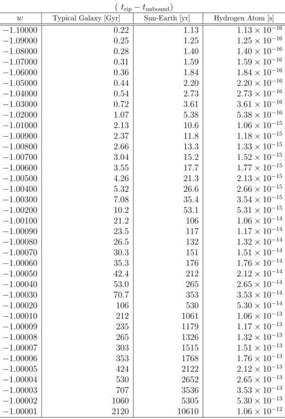
A.4 The formula for (trip−tunbound) . . . 42
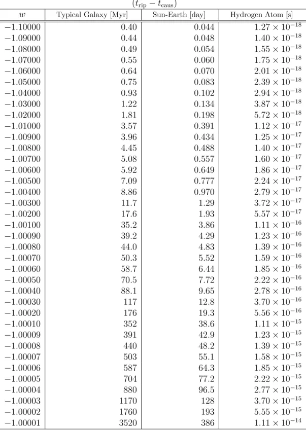
A.5 The formula for (trip−tcaus) . . . 48
VIII. APPENDIX C: COMES-BACK-EMPTY CONDITION . . . 54
IX. APPENDIX D: CONVENTIONS AND
ADDITIONAL BASIC FORMULAS . . . 56
LIST OF TABLES
Table
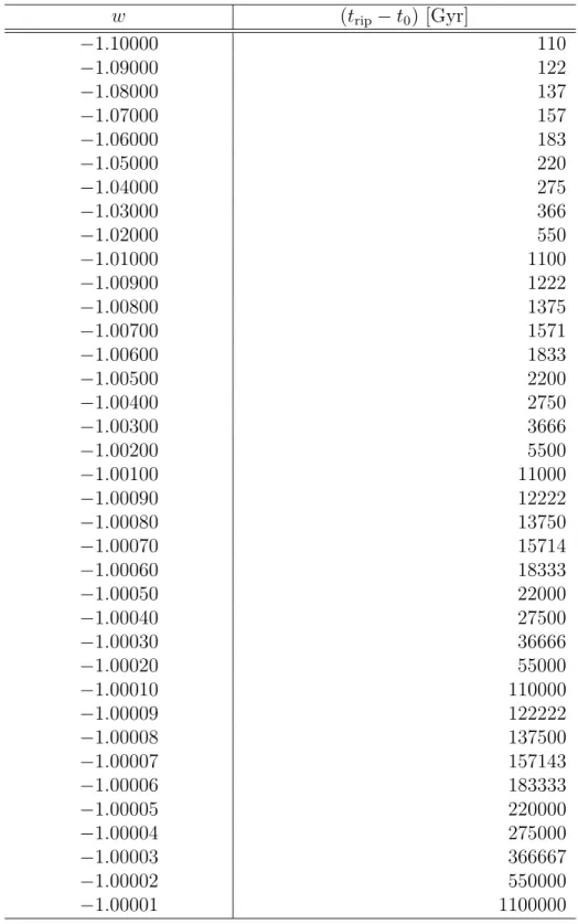
1. Values of (trip−t0) for−1.10000≤ω≤ −1.00001 . . . 40
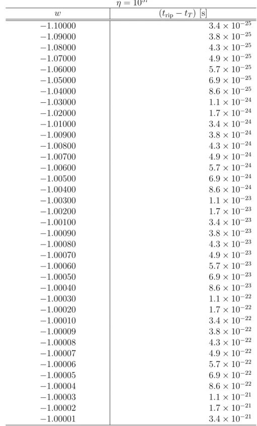
2. Values of (trip−tT) for−1.10000≤ω≤ −1.00001
with η= 1029 fixed . . . 43
3. Values of (trip−tT) for−1.10000≤ω≤ −1.00001
with η= 1057 fixed . . . 44
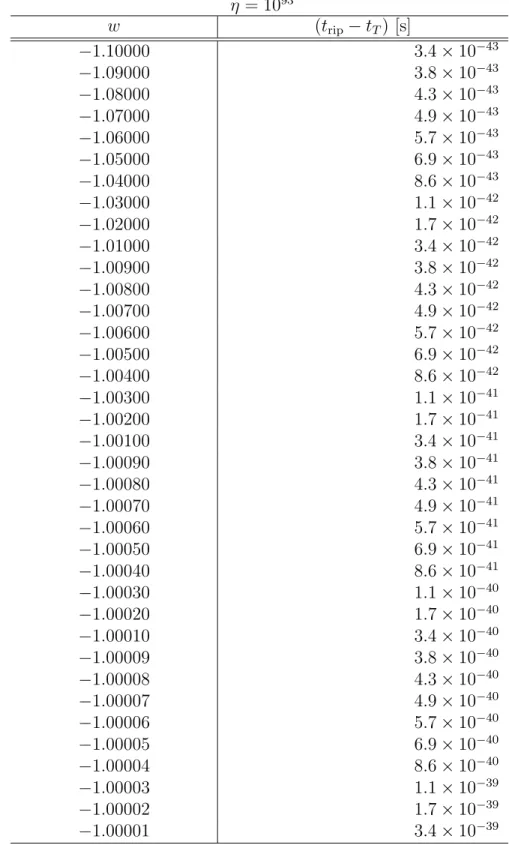
4. Values of (trip−tT) for−1.10000≤ω≤ −1.00001
with η= 1093 fixed . . . 45
5. Values of (trip−tunbound) for −1.10000≤ω ≤ −1.00001 . . . .49
LIST OF FIGURES
Figures
1. Constraint onw and Ncp coming from the CBE condition (Comes Back Empty), corresponding to inequality (28). The black band in this figure has been created by varying the length of smaller bound systems from Lp(t0) = 10−33m
to Lp(t0) = 10−15m; the bottom edge corresponds to the
lower value of Lp(t0). The region below the black band is
forbidden by the CBE condition. . . 34
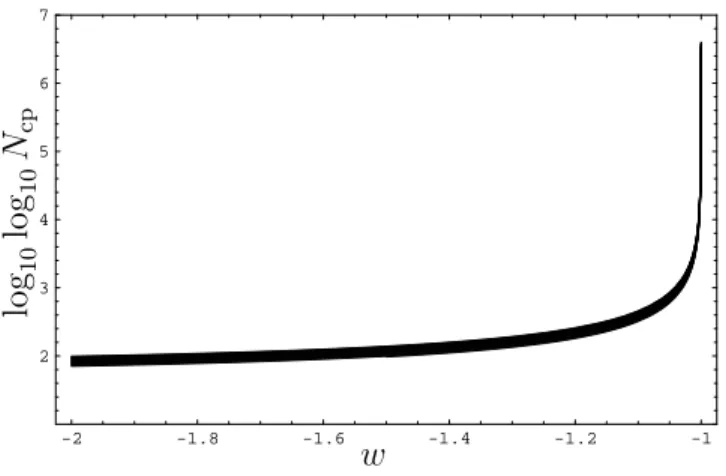
2. Constraint for −2≤w≤ −1.1 and Ncp coming from the CBE condition (Comes Back Empty), corresponding to inequality (28). The black band in this figure has been created by varying the length of smaller bound systems from Lp(t0) = 10−33m to Lp(t0) = 10−15m; the bottom
edge corresponds to the lower value of Lp(t0). The
region below the black band is forbidden by the
CBE condition. . . 35
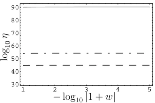
3. The lower bound on η coming from the causal disconnection conditions, tT > tHcaus (dashed line), tT > tNcaus (dashed-dotted line), tT > tPPPcaus (solid line), for 1029≤η≤1093 and −1.10000≤w≤ −1.00001. The regions below these three lines are forbidden
CHAPTER 1
INTRODUCTION
1.1 General Background
One of the longest standing issues in cosmology has been what is the overall
nature and history of the universe in the broadest sense? Did it spring forth from
one initial big bang? Has it always existed more or less as it is today? Or has it
perhaps gone through an infinite cycle of expansions and contractions? Or something
altogether different?
In 1916, Albert Einstein published his theory of general relativity containing
the famous Einstein equation (Gµν ≡ Rµν− 12Rgµν) = 8πGTµν. One of the popular
assumptions of the time, based on the general observational data available and the lack
of understanding of what nebulae actually were, was the notion of a static and largely
uniform universe. When Einstein began to look into the implications of his equation
for the universe as a whole, he quickly realized that it was not possible to obtain
a static solution with a uniform distribution of matter so, in 1917, he introduced a
cosmological constant term Λgµν into his field equation to get (Gµν−12Rgµν) + Λgµν =
8πGTµν (taking Λ = 8πG̺in order to balance out the attractive force of gravity) and
created a static, closed model of the universe. However, this proposal did not turn
out to be tenable as it was unstable to even the smallest of perturbations and it was
ruled out by later astronomical data which revealed an expanding universe.
Interestingly, over two centuries earlier similar discussions had occurred based
upon Newtonian theory. In 1692 Richard Bentley gave the first series of Boyle
must be infinite if it was to have any chance of not collapsing into a point due to the
force of gravity (although they were wrong because under Newtonian gravitation an
infinite universe would actually collapse back on itself in the same time as a finite
universe would) [1]. Furthermore, they agreed that it would have to be perfectly
arranged otherwise even the smallest perturbation would lead to collapse. Newton
concurred with their findings. Later in 1917, Willem de Sitter introduced an
alterna-tive construction for a static universe making use of the cosmological constant. His
model contained no matter at all, much to the consternation of Einstein who had
originally hoped that his theory of general relativity would have a single unique
so-lution that was our universe. It was not until six years later that Arthur Eddington
and Hermann Weyl were to discover that serious confusions (perhaps aided by the
prejudice of the day for a static universe) had led to the mistaken conclusion that de
Sitter’s model actually represented a static universe when it was, in fact, a model of
an expanding universe [1]. After considerable initial interest, de Sitter’s theory
even-tually fell by the wayside as the static universe was disproven and the mass density
was radically too low to be realistic. It did not re-emerge until decades later when,
in 1980, interest began in inflationary theory.
In 1922 mathematician and meteorologist Alexander Friedmann came up with
his famous solutions to the Einstein equation [2]. For calculational simplicity he took
the universe to be homogenous and isotropic, neither of which appeared to be
obser-vationally troubling. In his 1922 paper he discovered cases for expanding universes
having closed spatial geometries. In some of these cases the universe would expand to
a maximum size before turning around and crunching back into a point. In a second
paper, in 1924, he found cases for infinite open universes having a hyperbolic
geome-try which are know as the Friedmann world models. From the time-time component
of the Einstein equation came the the Friedmann equation (a˙
a)
2 + κ
a2 = 8πG3 ̺
H ≡ aa˙) and from the space-space components came 2aa¨ + (aa˙)2+ κ
R2 =−8πG̺where
a(t) is the scale factor for the expansion,κcharacterizes the geometry of the universe
and is usually normalized to ±1,0 (κ=−1 ⇔open, κ = 0 ⇔f lat, κ = 1⇔ closed)
and ̺is the total energy density. Taking the difference between the two equations of
Friedmann provides an equation for the acceleration: ¨a a =−
4πG
3 (̺+ 3p). Paired with the Robertson-Walker spacetime metric ds2 = −dt2+a2(t)[ dr2
1−κr2 +r2dΩ2], we have
the Friedmann-Roberston-Walker (FRW) model of the universe. If we include and
separate out the cosmological constant term, the Friedmann equation gets modified
to (aa˙)2+ κ
a2 = 8πG3 ̺+ Λ3. We can also provide a measure of the rate of change of the
expansion, known as the deceleration parameter, q = −a¨a
˙
a2. Although he did not
in-vestigate the particular case, at a certain critical density the limiting case of his open
hyperbolic or closed models produces a flat Euclidean model of infinite extent. The
FRW model was not generally given much regard at first since most data appeared
to show a generally static universe, but this would soon change.
In fact, there had already been hints. In 1868, Sir William Huggins had noted
a Doppler shift appearing in some starlight. Then in 1912, Vesto Melvin Slipher had
obtained data showing that spiral nebulae were red-shifted in a way consistent with
expansion, however, since nobody knew what the nebulae were and nobody imagined,
in particular, that they were actually distant galaxies, the data were not given much
thought (although as far back as the 18th century some, such as Kant, Lambert,
Swedenborg, and Wright, actually had philosophized that perhaps these nebulae were
actually distant galaxies much like our own). Furthermore, Arthur Eddington already
recognized in 1923 that Slipher’s data would fit in with an expanding de Sitter model
universe.
During the mid to late 1920’s, astronomers began taking general notice that the
nebulae were red-shifted. When Sir Edwin Hubble discovered the Cepheid variables
time that the spiral nebulae were in fact extra galactic systems and thus settled at
least the second half of what had become known as ‘The Great Debate’- what is
the size of our galaxy and are the spiral nebulae members of our galaxy or separate
‘island universes’ well beyond it? This led the Belgian civil engineer, priest and later
astrophysicist Georges Lemaˆıtre, in 1927, to independently derive the Friedmann
solutions (they were not yet widely known) and to propose that the universe might
not fit the static model but might instead have burst forth from a primeval atom.
This was the original big bang proposal. None of Lemaˆıtre’s models for the Big Bang
universe ultimately provided useful though as he ended up having to construct highly
convoluted models in order to force them to be in agreement with both observational
data for the age of the universe and an early and highly erroneous value for the Hubble
constant which was off by an order of magnitude [1].
A couple of years later, in 1929, Hubble announced that almost all galaxies (the
neighboring Andromeda is a notable exception) were moving away from us faster the
farther away from us they were and that they were all receding away from each other.
Then, in 1931, he went on to demonstrate this with data and Eddington brought
to general light Lemaˆıtre’s work. It was then that the expanding universe solutions
of the Friedmann equations finally began to attract considerable attention. One of
the Eddington/Lemaˆıtre models described a closed but ever expanding universe that
started out as an Einstein static universe and then later expanded at an ever increasing
rate due to the presence of a positive cosmological constant. As objects within this
universe were ultimately being expanded away from one another at faster than the
speed of light, Eddington believed that the galaxies would eventually become casually
disconnected from one another, each forming their own separate island universe [1,3].
Such ideas soon fell out of fashion since there was not even a hint of observational
evidence suggesting the possibility, but they were to awaken again decades later when,
It now appeared as if though the universe might be a dynamic one in which
wherever one stood it would look as if everything else was receding away in all
direc-tions. Astronomers characterize the redshift of distant objects by z= λobserved−λemitted
λemitted
with λemitted the wavelength of the light as emitted by the source and λobserved the
wavelength of the light when it reaches the Earth. The scale factor of the universe at
the time (t1)light was emitted from an object of redshift z is given by a(t1) = 1+1z. In
the special relativistic Doppler shift formula one gets 1+z = (1+vc 1−vc)
1
2 and although the
Doppler shift deals with relative velocity between two objects, the redshift is usually
thought of as a Doppler shift in the sense that the wavelength as we receive it may
appear to be longer or shorter than it was as it was emitted from the object. Some
suggest to interpret it as infinite sums of infinitesimal shifts along the path [4]. For
galaxies that are not too far off, astronomers can ignore the complications of general
relativity and simply use v = cz or, for the Hubble law, v =Hd where d(t) = a(t)r
withr being the co-moving radial coordinate andd(t) taken as the physical distance.
This gives the linear formula whereby a galaxy’s recession velocity is proportional to
its distance to us. The value of H at the present time isH0 ≃70km/s/Mpc.
It was at this time that Einstein suggested to remove the cosmological constant
from his equation and told George Gamow that the greatest blunder of his life had
been inserting it into his equation. However, the saga of the cosmological constant
was far from over. It was resurrected in the 1940’s and 1950’s when it was discovered
that the Hubble time was not consistent with the age of the Earth (producing an
Earth older than the universe itself!). The cosmological constant was removed again,
however, when it discovered that Hubble’s original estimate of his constant had been
off by an order of magnitude and the Hubble time actually had been consistent
to begin with, although this was still not the last that was to be heard from the
cosmological constant. It was ultimately discovered that it was a natural part of the
it to have either a massively large value or, through some method of cancelation, a
value of zero; anything but the vanishingly small and yet non-zero value that it is
now known (since 1998) to have.
After the discovery of the expansion of the universe by Hubble, two main
models for the universe emerged, the Steady State and the Big Bang.
The Big Bang model, which was promoted and expanded upon by Gamow,
was a model of a dynamic, changing universe which started out as a singularity and
then burst force across the entire volume of the universe from a primordial explosion
after which it went on to pass through a very hot radiation dominated stage before
proceeding to a matter dominated phase. In 1948, Gamow’s coworkers Raplh Alpher
and Robert Herman predicted, from their model, that there should exist a cosmic
microwave background (CMB) radiation of about 5K leftover from the cooling of
the surface of last scattering of the CMB (about 400,000 years after the alleged Big
Bang). At this time the universe was cool enough for electrons and protons to combine
into atoms and change from an opaque plasma to its present neutral and therefore
transparent form.
On the other hand, in the Steady State model of Fred Hoyle, Thomas Gold,
Hermann Bondi and others, new matter would be continually created as space
ex-panded so that the universe would be, overall, time independent. This model met the
Perfect Cosmological Principle which states the universe is homogenous and isotropic
in both space AND time (on the largest scales, the universe has a surprisingly
uni-form distribution of matter and looks now the same as it always has and always will).
Hoyle proposed a new C-Field that would have negative pressure to drive the
expan-sion and that would also create new matter. Hoyle despised the Big Bang model and
yet, ironically enough, was responsible for giving it its moniker, derisively referring
to it as “that big bang idea” on various BBC programs and lecture series throughout
More recently, Andrei Linde tried to invoke eternal inflation featuring
self-reproducing universes in order to avoid a beginning [5, 6]. However, Arvind Borde
and Alexander Vilenkin demonstrated that a reasonable spacetime that eternally
inflated into the future had to posses an initial singularity [7]. The idea was revisited
by Aguirre in 2002 [8, 9]. In more modern forms, eternal inflation or chaotic inflation
models of the universe have been introduced which while on smaller scales appear
more in line with the Big Bang model appear to have similarities to the Steady State
models when viewed on the grandest scales.
At first the community was split about fifty-fifty between the two competing
models (the Big Bang and the Steady State), but by the 1960’s the community had
shifted largely behind the Big Bang model as more and more astronomical data
hinted at a dynamic universe. For instance, quasars, seemed to show up in only very
ancient galaxies. By 1964 it was realized that stellar production could never give
the twenty-four percent by mass helium that was being seen throughout the universe
while primordial nucleosynthesis could; this was actually shown by the calculations
of Fred Hoyle and Roger Tayler in their 1964 paper in ‘Nature’.
In early 1964 came a revolutionary event when two Bell Labs radio astronomers,
Arno Penzias and Robert Wilson, just out of nearby Princeton graduate school, found
a pesky 2.7K source of systematic error in the experiment they were carrying out at
the Holmdel, NJ Bell Labs facility. By chance at a meeting they ran into someone
familiar with work going on at Princeton and had it suggested to them that they get
into contact with the gravitational physics group led by Robert H. Dicke.
Dicke was working on an oscillatory model for the universe and also
indepen-dently arriving at the idea of a relic cosmic background radiation. Also a member
of the group was Jim Peebles who worked out a clear prediction for a blackbody
spectrum for the CMB in 1965 (they later came across Gamow’s earlier little known
and Wilson that is was the CMB that they had discovered (beating out the Princeton
group’s Peter G. Roll and David T. Wilkinson who had been setting up their own
experimental search at the time).
This was, for the most part, the death knell for the Steady State models
although there were still some further variants such as Zwicki’s tired light model and
the Quasi-steady State model introduced by Fred Hoyle and others in 1993. Both
appeared problematic and never caught on.
The Penzias-Wilson discovery had an impact on competing Big Bang models
as well. The uniformity of the CMB allowed it to rule out Oskar Klein and Hannes
Alfven’s localized explosion model for the Big Bang [1].
1.2 Cyclic Universe Background
However, one important class of cosmological model, of an entirely different
nature, has been skipped over so far.
In the early 1930’s, Tolman proposed an oscillatory model for the universe [10].
He, along with many others over the years, didn’t like the idea of having an initial
singularity or the requirement for initial conditions, both inherent with the Big Bang
model, and considered the possibility of an ever existing, past and future complete,
infinite cyclic cosmology. His proposal was based upon a mechanism naturally
pro-vided by a “closed” universe which provides a turnaround point after the universe
has grown to a certain size, leading then to collapse back in on itself. The cyclic idea
is it will then spring forth again and repeat an infinite number of times.
Tolman carried out the earliest extensive work on cyclic universes [10, 11] and
was for long their most ardent supporter although various others such as Markov and
Dicke extensively investigated such models over the years too. However, these models
First, there is the second law of thermodynamics which leads to an entropy
conundrum. The entropy of the universe would increase with each cycle. Since the
greater the entropy in the universe the greater the maximum radius reached before
turnaround, each cycle would grow larger and longer than the previous one. Thus
tracing back in reverse from the current day one would get led back through ever
smaller cycles until one reached a singularity, exactly what one had hoped to avoid
[12]. These models of the universe would thus be future complete but could not be past
infinitely cyclic. Second, even if the entropy conundrum were not present, there would
still be the issue whereby large scale structure and black hole formation would lead to
serious problems during the contracting phase. For instance, black holes could grow
so large and copious during the contracting phase that it would cause a premature
bounce or cause the equations to break down. Finally, mix-master issues can occur
during the contracting stages which will cause wild oscillations of scale differentially
along the dimensions of space and create serious anisotropy issues [13–16]. On a side
note, in the late 1960’s Charles Misner tried unsuccessfully to use mix-master effects
to his advantage to get around the problems of causality and the uniformness of the
CMB for which inflation would later be proposed [14].
Ultimately, all of these early cyclic models were dropped as being futile. The
Big Bang emerged as the clear consensus model and, for all intents and purposes,
all cyclic cosmological models appeared to be dead. There was a brief revival of
such models by Markov in early to mid 1980’s [12, 17] but they also proved to be
problematic and the work on cyclic models was more or less abandoned once again.
However, extra-dimensional theories slowly began coming into vogue again, such as
String Theory, and then, in 1998, interesting astronomical data came to light [3] which
would revolutionize physics. It appeared as if most of the universe was currently made
up of an unknown energy called dark energy that was causing the universe to enter
At least since the time of Theodor Kaluza and Oskar Klein in the 1920’s, there
has been serious speculation that perhaps there are more dimensions than one of time
and three of space (in fact Gunnar Nordstrom, in 1914, had already attempted to
make use of an extra dimension when attempting to formulate his own theory of
gravitation and combine it with electromagnetism [18]). In 1921, Kaluza proposed a
theory [19] using an extra dimension of space, a 5th dimension, in an attempt to unify
Einstein’s theory of gravitation with Maxwell’s electromagnetism. Miraculously, by
simply adding an extra fifth dimension to Einstein’s theory of gravitation it
automati-cally produced the Maxwell equations of electromagnetism in addition to the Einstein
equations for gravitation! However, since we don’t observe any extra dimensions they
must be hidden and their effects suppressed in some way.
In 1926 Klein proposed [20] that the extra 5th dimension might be a
compact-ified dimension, a circular extra dimension appearing at each point in three
dimen-sional space, this becoming known as Kaluza-Klein reduction or compactification.
Imagining for simplicity only one instead of three standard spatial dimensions, the
extra compactified dimension cam be envisioned like a garden hose of vanishingly
small radius. Klein thereby solved the problem of why the extra dimension’s effects
appeared to be suppressed and why we don’t notice them. Additionally, it explained
why the electric charge is quantized [21].
However, Kaluza-Klein unification would not be the end of the story for
nu-merous technical issues not to mention entirely new forces and particles which came
to light. For decades it was thought that the only way in which extra dimensions
could tenably arise was through compactification into exceedingly small size.
However, in 1998 Nima Arkani-Hamed, Savas Dimopoulos, and Gia Dvali
(ADD) proposed a new model in an attempt to explain the relative weakness of
gravity compared to the other forces. The ADD model made use of large,
introduced their “RS1” model featuring two branes and a large, warped extra
dimen-sion [23]. Shortly afterward, they introduced their “RS2” model which contained an
extra dimension that was not only not compactified, but actually infinite in extent
as they sent the second brane in RS1 to infinity [24]. From the five-dimensional RS
model one can obtain an effective modified Friedmann equation in four-dimensions
that contains a new̺2 (̺≡density) term in addition to the usual ̺term. This form
of modified Friedmann equation is not actually specific to this particular model but
more general [25].
In braneworld scenarios like RS1 one takes the standard model particles to be
constrained within a hyper-surface brane that lies within a higher-dimensional bulk.
Gravity (and perhaps exotic particles) can travel throughout the bulk. Such models
can arise, for instance, from within string theory such as through the strong coupling
limit of the E8XE8 Horava-Witten model [26]. Compacting six of eleven dimensions
onto a Calabi-Yau manifold leaves an effectively five-dimensional spacetime with two
four-dimensional boundary branes. In many models featuring two such branes, with
the standard particles confined to one of the two, changing the moduli controlling
the distance between the two branes within the bulk can effectively look, in
four-dimensions, like an expansion or contraction of space. For example, in the RS models,
if the brane moves as a function ofw(t) this induces a FRW scale factor ofa(t) =e−k|w|
[27, 28]. In some models the brane separation needs to be constrained to provide the
proper spectrum of standard model particles and forces [25, 29, 30].
Also totally unexpected were the implications of new astronomical
observa-tions carried out in the late 1990’s. In 1998 it was announced that the expansion
rate of the universe was actually increasing at the current time instead of remaining
constant or slowing down [3]. This was an entirely unexpected finding. The cause
for the increasing expansion rate became referred to as dark energy. Dark energy is
which goes as ̺ ∝ a−3(1+w) in the Friedmann equation. More specifically, ̺ goes,
depending upon whether it is radiation, matter, vacuum energy, or phantom energy
as:
radiation: p= ̺3 ⇒ ̺∝ 1
a4
matter: p=0⇒ ̺∝ a13
vacuum energy: p=−̺ ⇒ ̺∝constant
phantom energy: p <−̺ (taking, for one example, p=−43̺ ⇒̺∝a)
with the latter phantom form capable of eventually leading to exceptional causal
structure as will be employed in this dissertation.
With the discovery of dark energy and it’s potentially exotic nature, and with
renewed interest in extra-dimensions and the ensuing braneworlds and other
con-structions, it became natural to wonder if there might not be some way around the
problems which had derailed prior attempts at constructing consistent cyclic models
of the universe. Might the cyclic universe not be opened up again to possibility?
Work attempting to use some of the new possibilities began again, for instance
in a 2001 model without the need for inflation, the Ekpyrotic model [31]. Bouncing
braneworlds with an extra dimension of time such as [32] began to be investigated.
Also making use of branes and phantom energy [33], which examined the consequences
for cyclic cosmology.
After their initial Ekpyrotic model, Steinhardt and Turok began working on
a derivative model [34–42] which could avoid a big bang and thereby made progress
towards a cyclic model (although without resolving the entropy conundrum [43]).
1.3 Outline of a Cyclic Model
The rise of dark energy, only discovered in 1998 [3], proves to be a crucial
of state is w <−1 (current observations are centered around −1 with some slightly
favoring w <−1 [44]) then the universe may eventually enter a period of exceptional
causal structure. Within the realms of models following the standard Friedmann
equation, such a phantom dark energy would eventually lead to a Big Rip within a
finite amount of time and tear apart the fabric of spacetime [45].
The Big Rip and replacement of dark energy by modified gravity were explored
further in [46,47]. If one turns to a modified Friedmann equation (H2 = 8π
3M2
p(̺−
̺2
2σ))
where σ is a brane tension then at ̺b = 2|σ| one finds H = 0 as required at a
turnaround or bounce in cyclic cosmology. Such can arise in a variety of models, the
Big Rip can be avoided as well as any crunch to a singularity at the other end of the
cycle.
It is such ideas coupled to dark energy that provide new avenues to travel
down in the hopes of being able to construct cyclic models of the universe which may
be both future AND past complete.
We consider here a model where just before reaching the Big Rip a brane
contribution creates a turnaround at which time the scale factor deflates to a very
tiny fraction (f) of itself and only one casual patch is retained, while the other f13
patches independently contract to separate universes.
The universe is causally fractionated into a tremendous number (more than
one googol, 10100) of independent patches. Contraction occurs with a much smaller
universe which returns almost empty and eventually bounces just before a singularity
would be hit and then enters into a brief period of standard inflationary expansion.
Inflation injects a huge amount of entropy and so begins the next generically
iden-tical cycle and the new idea of how to overcome the seemingly impossible entropy
CHAPTER 2
TURNAROUND IN CYCLIC COSMOLOGY
2.1 Basics of Model
If the dark energy has a super-negative equation of state, ωΛ = pΛ
̺Λ < −1,
it leads to a Big Rip [45, 48] at a finite future time where there exist extraordinary
conditions with regard to density and causality as one approaches the Rip. We next
explore whether these exceptional conditions can assist in providing an infinitely cyclic
model.
We consider a model where, as we approach, expansion stops just short of the
Big Rip due to a brane-like contribution. There is a turnaround at timet =tT when
the scale factor is deflated to a very tiny fraction (f) of itself and only one causal
patch is retained, while the other 1/f3 patches contract independently to separate
universes. Turnaround takes place an extremely short time (< 10−27s) before the
Big Rip would have occurred, at a time when the universe is fractionated into many
independent causal patches [47].
There follows contraction which occurs with a very much smaller universe than
in expansion and with almost vanishing entropy because it is assumed empty of dust,
matter and black holes and where even photons have become infinitely redshifted.
On the other end of a cycle, a bounce takes place a short time before a crunch
into a singularity would have occurred (based on present day knowledge). After the
bounce, entropy is injected by inflation [49], where it is assumed that an inflaton field
the work of [34–37]. For cyclicity of the entropy (S(t) =S(t+τ)) to be consistent with
thermodynamics it is necessary that the deflationary decrease by f3 will compensate
for the entropy increase acquired during expansion including during inflation.
A possible shortcoming of the proposal could have been the persistence of
spacetime singularities in cyclic cosmologies [43], but to our understanding for the
model we outline this problem is avoided (provided that the time average of the
Hubble parameter during expansion is equal in magnitude and opposite in sign to its
average during contraction).
2.2 Friedmann Equation for Expansion Phase
Let the period of the Universe be designated by τ and the bounce take place
at t = 0 and turnaround at t = tT. Then we have the expansion phase for times
0 < t < tT and the contraction phase corresponds for times tT < t < τ. We employ
the following Friedmann equation for the expansionperiod 0< t < tT:
˙ a(t) a(t) 2 = 8πG 3
(̺Λ)0 a(t)3(ωΛ+1) +
(̺m)0 a(t)3 +
(̺r)0 a(t)4
− ̺total(t)
2
̺c
(1)
where the scale factor is normalized to a(t0) = 1 at the present time t=t0 ≃14Gy.
To explain the notation, (̺i)0 denotes the value of the density ̺i at timet=t0. The
first two terms are the dark energy and total matter (dark plus luminous) satisfying
ΩΛ=
8πG(̺Λ)0 3H2
0
= 0.72 and Ωm =
8πG(̺m)0
3H2 0
= 0.28 (2)
where H0 = ˙a(t0)/a(t0). The third term in the Friedmann equation is the radiation
density which is now Ωr = 1.3×10⁻⁴. The final term ∼̺total(t)2 is derivable from a
braneworld construct [23,24,33,50]; we use a negative sign naturally arising from
neg-ative brane tension (the negneg-ative sign can arise also from a second time-like dimension
As the turnaround is approached, the only significant terms in Eq.(1) are the first
(where ωΛ < −1) and the last. As the bounce is approached, the only important
terms in Eq.(1) are the third and the last. (We shall later argue that the second
term, for matter, is absent during contraction.) In particular, the final term of Eq.
(1), ∼ ̺total(t)2, arising from the braneworld construct is insignificant for almost the
entire cycle but becomes dominant as one approaches t→tT for the turnaround and
again for t→τ as once approaches the bounce.
2.3 Turnaround
Let us assume for algebraic simplicity that ωΛ = −4/3 = constant. This
value is already almost excluded by WMAP3 [51] but to begin we are aiming only at
consistency of infinite cyclicity. More realistic values are left for future investigation.
With the value ωΛ =−4/3 we learn from [46] that the time to the Big Rip is (trip−
t0) = 11Gy(−ωΛ −1)−1 = 33Gy which is, as we shall discuss, within 10−27 second
or less of when turnaround occurs at t = tT. So if we adopt t0 = 14Gy then tT =
t0 + (trip−t0) ∼ (14 + 33)Gy = 47Gy. From the analysis in [45–48] the time when
a system becomes gravitationally unbound corresponds approximately to the time
when the dark energy density matches the mean density of the bound system. For
an object like the Earth or a hydrogen atom, water density ̺H2O is a practical unit.
With this in mind, for the simple case ofω=−4/3 we see from Eq.(1) that the
dark energy density grows proportional to the scale factor ̺Λ(t)∝ a(t) and so given
that the dark energy at present is ̺Λ ∼10−29g/cm3 it follows that ̺Λ(t
H2O) =̺H2O
when a(tH2O) ∼ 10
29. We can estimate the time t
H2O by taking on the RHS of the
Friedmann equation only dark energy aa˙2
=H2
0ΩΛa−β with β = 3(1 +ω). When we
specialize to ω =−4/3 it follows that
a(tH2O)
(a(t0) = 1) =
(trip−t0)
(trip−tH2O)
2
so that (trip−tH2O) = 33Gy×10
−14.5 ≃ 103.5s ∼ 1 hour. [The value is sensitive to
ω.] It is instructive to consider an approach to the Rip using a more general critical
density̺c =η̺H2O and to compute the time (trip−tη) such that̺Λ(tη) =̺c =η̺H2O.
We then find, using a(tη) = 1029η, that#1
(trip−tη) = (trip−t0)10−14.5η−
1 2 ≃η−
1
2hours (4)
which is the required result. We shall see thatη >1031so the time in (4) is<10−27s.
To discuss the turnaround analytically we keep only the first and last terms,
the only significant ones, on the RHS of Eq.(1) which becomes for the special case
ω = 4/3
˙ a a
2
=α1a−α2a2 (5)
in which
α1 = 8πG
3 (̺Λ)0 α2 = 8πG
3
(̺Λ)20 ̺c
(6)
Writing a =z2 and z = (α1/α2)1/2sinθ gives
dt= 2
√α
2 α1
dθ sin2θ =
2√α2 α1
d(−cotθ) (7)
Integration then gives for the scale factor
a(t) =
α1 α2
sin2θ = ̺c (̺Λ)0
"
1 1 + tT−t
C
2 #
(8)
where C = −(3/2πG̺c)1/2. At turnaround t = tT, a(tT) = [̺C/(̺λ)0] = (a(t))max.
At the present time t=t0, a(t0) = 1 andsin2θ0 = [(̺Λ)0/̺
C]≪1, increasing during
subsequent expansion to θT =π/4.
A key ingredient in our model is that at turnaround, t = tT, our universe
deflates dramatically with an effective scale factora(tT) shrinking before contraction
to ˆa(tT) =f a(tT) wheref <10−28. This jettisoning of almost all, a fraction (1−f), of
the accumulated entropy need be permitted by the exceptional causal structure of the
universe in some fashion. We shall see later that the parameter η at turnaround lies
in the rangeη= 1031 toη = 1087 which implies a dark energy density at turnaround
(Planckian density of ̺Λ ∼ 10104̺
H2O can be avoided) such that, according to the
Big Rip analysis of [46,47], all known, and yet unknown smaller, bound systems have
become unbound and the constituents causally disconnected. Recall that the density
of a hydrogen atom is approximately̺H2O and we are reaching a dark energy density
of from 31 to 87 orders of magnitude higher.
According to these estimates, at t = tT the universe has already fragmented
into an astronomical number (1/f3) of causal patches, each of which independently
contracts as a separate universe leading to an infinite multiverse. The entropy at
t = tT is thus divided between these new contracting universes and our universe
retains only a fraction f3. Since our model universe has cycled an infinite number of
times, the number of parallel universes is infinite.
2.4 Deflation
A central assumption in our cyclic model is that almost all of the entropy is
jettisoned at turnaround by the retention of one causal patch. We cannot justify this
step rigorously but hope to convince the reader by the following physical argument.
Let us take a bounce temperature TB = 10p GeV with p >3. This gives (see below)
η= 10(19+4p) and hence, from Eq.(4), (t
rip−tT)∼10−(19+4p) hours. The dark energy
density̺c ∼10(19+4p)g/cm3at turnaround implies the prior disintegration of all bound
systems with mean density ̺ < ̺c, which for p > 3 includes atoms, nuclei, nucleons
(1015g/cm3) and even smaller bound systems, if any. As shown in [45, 46, 48], at a
causally disconnected. For such a density, a generic causal patch contains no quarks
or leptons, only dark energy together with a small number of highly infra-red photons.
Black holes are also absent, having been torn apart by the approach to the would-be
Big Rip e.g.[33]. The entropy of such a patch is essentially zero, by which we mean
S = O(101) compared to the earlier S > 1088. This dramatic decrease in entropy
is called deflation for obvious reasons. During contraction, as we shall describe, the
entropy remains constant at essentially zero because dark energy has zero entropy and
radiation contracts adiabatically. Although these heuristic arguments about deflation
seem clear, a more rigorous justification would certainly be most desirable.
2.5 Friedmann Equation for Contraction Phase
The contraction phase for our universe occurs for the period tT < t < τ. The
scale factor during the contraction phase will be denoted by ˆa(t) while we always use
the same linear time t subject to the periodicity t +τ ≡ t. At the turnaround we
retain a fraction f3 of the entropy with ˆa(t
T) = f a(tT). For the contraction phase,
the Friedmann equation is
˙ˆ a(t) ˆ a(t) !2 = 8πG 3
(ˆ̺Λ)0 ˆ
a(t)3(ωΛ+1) +
(ˆ̺r)0 ˆ a(t)4
−̺ˆtotal(t)
2
ˆ ̺c
(9)
where we have defined
ˆ ̺i(t) =
(̺i)0f3(ωi+1)
ˆ
a(t)3(ωi+1) =
(ˆ̺i)0
ˆ
a(t)3(ωi+1) (10)
In contrast to Eq.(1), however, we have set ˆ̺m = 0 because our hypothesis is that
the causal patch retained in the model contains only dark energy and radiation but
no matter (including no black holes). This is necessary because during a contracting
phase dust or matter would clump, even more readily than during expansion, and
matter would require that our universe go in reverse through several phase transitions
(recombination, QCD and electroweak to name a few) which would violate the second
law of thermodynamics. We thus require that our universe comes back empty! Note
that any tiny entropy associated with radiation will be constant during adiabatic
contraction.
The contraction of our universe will proceed from one of the 1/f3 causal
patches following Eq.(9) until the radiation balances the brane tension at the bounce.
2.6 Bounce
At the bounce, the contraction scale is given, using ̺c =η̺H2O, from Eq. (1)
as
a(τ)4 =
(̺r)0
η̺H2O
(11)
Now the model’s bounce att =τ must be before the electroweak transition attEW =
10−10s when a(t
EW) = 10−15, and after the Planck scale when a(tP lanck) = 10−32 in
order to accommodate the well established weak transition and to avoid uncertainties
associated with quantum gravity. With this in mind, here are three illustrative values
(A, B, C) for the bounce temperature TB:
• (A) At a GUT scale TB = 1017GeV, a(tB) = 10−30.
• (B) At an intermediate scale TB = 1010GeV, a(tB) = 10−23.
• (C) At a weak scale TB = 103GeV, a(tB) = 10−16.
From Eq.(11) and Eq.(4) for these three cases one finds
• (A)η = 1087 and (t
rip−tT) = 10−87hr.
• (A)η = 1059 and (t
rip−tT) = 10−59hr.
Immediately after the bounce, we assume that an inflaton field is excited
and there is conventional inflation with enhancement E = a(τ +δ)/ˆa(τ). Successful
inflation requires E >1028. Consistency requires therefore f < E−1 to allow for the
entropy accrued during expansion after inflation. The fraction of entropy jettisoned
from our universe at deflation is thus extremely close to one, being less than one and
more than (1−10−28)3.
2.7 Entropy
Consider first the present epoch t =t0. The contributions of radiation to the
entropy density s follow the relation
s = 2π 2
45g∗T
3 (12)
Photons contributeg∗ = 2. The present CMB temperature isT = 2.73K ≡0.235meV ∼
1.191(mm)−1. Substitution into Eq.(12) gives a present radiation entropy density of
sγ(t0) = 1.48(mm)−3. Using a volume estimate V = (4π/3)R3 with R = 10Gly ≃
1029mm gives a total radiation entropy of S
γ ∼ 6.3×1087. Including neutrinos
in-crease g∗ in Eq.(12) from g∗ = 2 to g∗ = 3.36 = 2 + 6×(7/8)×(4/11)4/3. This
increases Sγ = 6.3×1087 to Sγ+ν ∼ ×1088.
This total entropy is interpretable as exp(1088) degrees of freedom, or in
in-formation theory [53] to a number I of qubits where 2I = eS so that I = S/(ln2 =
0.693)∼1088. This is well below the holographic bound which is dictated by the area
in terms of Planck units 10−64mm2which givesS
holog(t0) = 4π(1029mm)2/(10−32mm)2 ∼
10123 or about 1035 times bigger. In [53] it is suggested that at least some of this
dif-ference may come from super-massive black holes. The entropy contribution from
baryons is smaller than Sγ by some ten orders of magnitude so, like that from the
What is the entropy of the dark energy? If it is perfectly homogeneous and
non-interacting it has zero temperature and entropy. Finally, as we have already
estimated, the fourth term in Eq.(1), corresponding to the brane term, is negligible.
The conclusion is that at present Stotal(t0)∼1088.
Now consider the entropy approaching turnaround at t = tT. We have
esti-mated thata(tT) = 1029ηand representative values forη=̺c/̺H2O are 10
31,1059and
1087. The temperatureT
γ of the radiation scales as Tγ ∝a(t)−1 so using the entropy
density of Eq.(12) a co-moving 3-volume∝a(t)3 will contain the same total radiation
entropy Sγ(tT) = Sγ(t0) as at present; this is simply the usual adiabatic expansion.
The expansion fromt = 0 totT is not purely adiabatic because irreversible processes
take place. The first is inflation which increases entropy by > 1084. There are also
phase transitions such as the electroweak transition at tEW ∼100ps, the QCD phase
transition at tQCD ∼ 100µs, and recombination at trec ∼ 1013s. Furthermore, there
are irreversible processes that occur during stellar evolution. Although the expansion
of the radiation, the dominant contributor to the entropy, is adiabatic, the entropy of
matter increases in accord with the second law of thermodynamics. In our model, the
entropy of the matter increases between t = 0 and tT ∼ 47Gy. Setting the entropy
of the dark energy to zero and with the the radiation acting adiabatically, it is the
matter part, represented by ̺m, which would cause the entropy to rise from S(t = 0)
to S(tT) = S(t = 0) + ∆S. It is this ∆S that was one of the plagues of previous
oscillatory model universes [2, 10, 11].
Our main point is that in order for entropy to be cyclic, the entropy which was
enhanced by a huge factorE3 >1084 at inflation must then be reduced dramatically
at some point during the cycle so that satisfying S(t) = S(t+τ) becomes possible.
Since entropy increases during regular expansion and contraction, the only logical
possibility is to have the decrease occur right at the approach to and at turnaround
of thermodynamics continues to obtain for other causal patches taken as a whole,
each with practically vanishing entropy at turnaround, but these are permanently
removed from the consideration of any particular universe under inspection, as they
all contract instead into separate universes.
During contraction, tT < t < τ, we are assuming the universe is empty of
matter until the bounce so its entropy is vanishingly small. Immediately after the
bounce, inflation arises from an inflaton field, assumed to be excited. We find the
counterpoise of inflation at the bounce and deflation at turnaround an appealing
aspect of the present model. And this would be furtherso, were the phantom dark
energy and inflaton be related or interacting, especially in a self-perpetuating manner.
2.8 Conclusion
The standard cosmology based on a Big Bang augmented by an inflationary
era is impressively consistent with the detailed data from WMAP3 [51] if dark energy,
most conservatively taken as a cosmological constant, is included. Objections to this
standard model are more aesthetic than motivated directly by observations (although
certain polarizations of the CMB, were they to be discovered, might well lead to some
discord). The first potential objection is the nature of the initial singularity and the
initial conditions. A second potential objection, if not universally shared either, is
that the predicted fate of the universe is an infinitely long expansion. Regardless of
whether or not one finds these issues more troubling than the nature of an infinitely
oscillatory cosmology, and there are many on either side of the aisle, we are driven by
the curiosity as to whether -and it is instructive to see as well- or not such a model
of the universe may even be possible even in theory. We have outlined here a cyclic
cosmology resting on phantom dark energy where these potential aesthetic objections
of some are ameliorated: the classical density and temperature never become infinite
to a multiverse picture, somewhat reminiscent of that predicted in eternal inflation
(and perhaps even including the infinities of eternal inflation within our model’s own
infinities). Here though our new proliferation of infinite universes originates at the
CHAPTER 3
ENTROPY OF CONTRACTING UNIVERSE IN CYCLIC
COSMOLOGY
3.1 Entropy
To recapitulate, the most important new ingredient in our model is the idea
that the contracting universe has essentially zero entropy and comes back empty of
matter. Taking this model seriously #2 we continue on to examine more critically
some general features including its possibility of being tested.
The contracting universe of the cyclic model contains phantom dark energy
with zero entropy and perhaps a small amount of radiation which could possess
en-tropy. The deflation at turnaround reduces entropy from a gigantic value O(>1088)
to an extremely low value O(101). We will next proceed to study the entropy of the
contracting universe in our speculative scenario more quantitatively, now taking an
arbitrary ω=−1−φ with φ >0 such that ̺Λ ∝a3φ.
The quantityφ is the most important parameter for observational
discrimina-tion between our cyclic model which takes dark energy to be phantom in nature and
one taking dark energy as the cosmological constant #3. The next test of φ 6= 0 will
likely come from the Planck Surveyor satellite [54]. One wonders, therefore, how
dif-ferent from zeroφ is? There is no lower bound necessary on φ for our model to work
other than it must be non-zero. We already know that φ . 0.1 from the WMAP3
#2It was once memorably stated by Noble laureate Steven Weinberg [55] that “the problem is not
that theorists take their model too seriously but that they do not take it seriously enough”.
data [51]. If φ is truly infinitesimal, the test must, alas, await improved technology.
To restore optimism, at the end of this section will be provided an anthropic fine
tuning argument demonstrating that an extremely small value for φ is unlikely.
We have emphasized that the universe comes back empty of matter, including
black holes. The presence of matter during contraction causes apparently
insuper-able problems because accelerated structure formation will precipitate a premature
bounce or lead to other even more dire issues. Black holes, if present, will expand
and proliferate with the same consequences. But the presence of radiation must also
be carefully studied because, although at turnaround the photon energy is
infinites-imal (Eγ . 10−200eV), the blue shifting during contraction leads to production of
e+e− pairs before the bounce. This is undesirable because, generically, they will
cre-ate problems with continued contraction. As we shall proceed to show, there are
fortunately no photons in the contracting phase of the cycle, only the presumably
innocuous dark energy.
Our cyclic model contains but one free parameter, ̺C, the common density at
which the universe both turns around and bounces. Since the bounce is independent
of ω, we begin with it and take as bounce temperatures TB = 10p GeV, so as to be
above the weak and below the Planck scales, with 3 ≤p ≤17. Using the derivation
from section 2, this gives ̺C =η̺H2O where η = 10
(19+4p) and ̺
H20 = 1g/cm
3 is the
density of water. The density of water being an easily imaginable unit somewhere
between the unimaginably small present mean cosmic density and the unimaginably
large critical density ̺C at turnaround and bounce.
Going now to the turnaround at time t=tT, the scale factora(tT) is given by
(since a(t0) = 1 and taking ̺0 = 10−29̺
H2O)
The present radiation temperature is (Tγ)0 = 2×10⁻⁴ eV, and so from Eq.(13) the
radiation temperature at turnaround is
(Tγ)T = 2×10⁻⁴ 10(48+4p)
−1/3φ
eV (14)
which is infinitesimal. Putting φ = 0.1, Eq.(14) gives 10−200 eV for p=3 and 10−390
eV for p=17; with φ= 0.01, the photon energy is 10−2000 eV for p=3 and 10−3900 eV
for p=17. In all cases, the photon wavelength is an astronomical number of orders of
magnitude longer than the present Hubble length.
To evaluate the entropy during contraction, we need to estimate how many
such photons there will be per causal patch at turnaround. The deflationary factor
multiplying entropy at turnaround must be much less than the inverse of the
infla-tionary increase (& 1084) of the early universe. We take the huge number of causal
patches to be 1090αwhereα≫1 is a parameter to allow an arbitrarily larger number,
and α= 1 will give an overestimate of the contraction entropy.
At turnaround the scale factor is
a(tT) = 10(48+4p)
31φ
(15)
so taking the present volume as 1084cm3 and the present radiation density to be
̺r(t0) = 10−33g/cm3 = 1eV /cm3 gives us the radiation energy in one causal patch:
(Er)patch=
1
(100α)3 10
(48+4p)−31φ
eV (16)
Comparison with Eq.(14) then gives the number of photons per causal patch
to be
nγ =
1
200α3 ≪1 (17)
Thus, the entropy of the contracting universe (cu) vanishes Scu = 0 for any value of
the equation of state of the dark energy ω = p/̺ =−1−φ since Eq.(17) has no φ
dependence.
3.2 Anthropic Fine Tuning Argument About
φ
The time until turnaround is given, e.g.[46], by
(tT −t0)≃
t0
φ (18)
so, if we take for simplicity the origin of life to have occurred at t0, after the most
recent bounce we see from Eq. (18) that given small φ ≪1 then φ will measure the
fraction of the expansion phase taken to originate life. An anthropic argument is: it
is unreasonable for the fraction φ, assuming it is non-zero, to be extremely close to
zero.
The special caseφ= 0 is the standard cosmological model with a cosmological
constant where there is no turnaround and the future lifetime is infinite so the origin
of life necessarily takes place after a vanishing fraction of the expansion lifetime. Such
an infinite expansion seems unaesthetic to some, but it is not a universal concern.
The vanishing fraction coincidence is puzzling however.
As soon as one commits to φ 6= 0, however, the anthropic type argument
emerges and it is unlikely thatφ <<<1. For example, ifφ= 10−3 then the length of
the expansion phase is 104 Gy whereas life originated after only about 10 Gy which
is only 0.1% of the expansion time. If life plays a central role in our universe, as in
our understanding is the spirit of the anthropic principle, such a tiny value of φ is
strongly disfavored; one expects at least φ&0.01 so the fraction before the origin of
life is&1.0% of the total expansion time.
This encouraging argument makes it more optimistic that the next generation
CHAPTER 4
CONSTRAINTS ON DEFLATION FROM THE EQUATION
OF STATE OF DARK ENERGY
4.1 Background
Our model involves two key ideas: (i) that the universe deflate just prior to
the turnaround from expansion to contraction by disintegrating into a very large
number Ncp of causal patches (in our notation, note that Ncp = 1/f3); (ii) that the
contracting universe be empty, meaning that one causal patch at turnaround must
contain no matter or black holes, only dark energy. This is called the CBE condition
(Comes Back Empty). Implementation of CBE requires, as we shall explain, a lower
bound onNcp which depends on the length scale Lcharacterizing the smallest bound
system. We shall consider both L = 10−15m for a nucleon then L ≥ 10−35m for a
PPP (Presently Point Particle) meaning a particle which at present is considered to be
point-like, such as a quark or lepton, but which might potentially have a characteristic
size greater than or equal to the Planck scale, if at least a few orders of magnitude
smaller than a nucleon.
In the foreseeable future, it is expected that the equation of state of dark energy
w, and hence φ, will be measured with higher accuracy by, for example, the Planck
Surveyor satellite [54]. What we shall show is that this measurement can, within this
model, constrain for a given w the number Ncp of causal patches at turnaround by
imposing a lower bound thereon.
In the present chapter, the times at which unbinding, causal disconnection and
of φ are derived followed by more discussion (also see Appendices A-C for more
technical material supplementing the main text here).
4.2 Times of Unbinding, Causal Disconnection and Turnaround
In this sub-section we analyze four relationships between cosmic times, in
addition to the present timet0, in the cyclic model expansion era: i)tunbound (at which
point a bound system will become unbound due to the large phantom dark energy
force with w < −1); ii) tcaus (at which point a previously bound system becomes
casually disconnected, meaning that no light signal could exchange before the
would-be Big Rip; this is how we estimate Ncp); iii) tT (at which point the turnaround
occurs); iv) trip (at which point a “would-be” Big Rip would have taken place).
There are three parameters: w (the equation of state of dark energy), ̺C (the
critical density when the total density in the system ̺tot is reached at t=tT), f (the
deflation fraction parameter related to the number of causal patches byNcp = (1/f3)).
We proceed to analyze the model taking w to lie within the range
−1.10000≤ω ≤ −1.00001, (19)
and ̺C within
(103GeV)4 ≤̺C ≤(1019GeV)4. (20)
The choice of the lower bound on the range ofwis motivated by current observations
[51, 56] while we are led to the upper bound by the cosmic variance uncertainty in
Reserving details of their derivation to Appendix A, we shall here refer to the resultant
expressions:
• (trip−t0)
trip−t0 ≃ 11 Gyr
|1 +w|. (21)
• (trip−tunbound)
trip−tunbound =α(w)P (22)
where [45]
α(w) =
p
2|1 + 3w|
6π|1 +w| (23)
and P denotes the period associated with the binding force which had been
constraining objects into a certain bound system beforet =tunbound.
• (trip−tcaus)
trip−tcaus =
1 + 3w 3(1 +w)
L c (24)
where c is the speed of light and L stands for the length scale of the bound
system [45].
• (trip−tT)
trip−tT =
11 Gyr
|1 +w|10
−14.5η−1
2 (25)
where η is a scale factor of ̺C defined by ̺C = η̺H2O with ̺H2O being the
density of water, ̺H2O = 1g·cm
The numerical analysis for these relationships is presented in Appendices A and B.
As a result, we find the lower bound for̺C,
̺C &(1018GeV)4, (26)
which is obtained by imposing that a presently point particle (PPP), having a size
10−33m = L, satisfy for time: t
rip > tT > tPPPcaus > tPPPunbound. It should be emphasized
that this result is almost independent of the choice ofw within the range of interest.
For a nucleon with L≃10−15m, the corresponding lower bound is
̺C &(109GeV)4. (27)
4.3 Given
w
, the constraints on
N
cpIn the chapter, as in [45], various bound systems have been discussed including
galaxies, the Earth-Sun system, the hydrogen atom and a nucleon. Each may be
characterized by a present length scale L0.
For the CBE condition we must insist that the smallest bound systems, whose
present length scale is L(t0) =L0, are disintegrated before turnaround which means
that the size of a generic causal patch Lcp (to be defined below) must be smaller than
L(tT) at the turnaround, namely
Lcp ≤L(tT) =L0
a(tT)
a(tunbound)
. (28)
We remind the reader that the CBE condition is mandatory because if the
contracting universe contains matter it will not generally contract sufficiently and will
undergo a premature bounce. Even if a causal patch contains only one very infra-red
bounce, again disallowing sufficient contraction for infinite cyclicity.
We have already demonstrated that the mean number of low-energy photons
per causal patch is very much less than one and therefore almost every patch contains
no photons. There will always be a vanishing but strictly non-zero number of patches
which fail to cycle but it can clearly be seen that this will not overwhelm the overall
infinity and will not ruin the model as was verified by direct calculation in [57, 58].
The probability of a successful universe is equal to one. The total number of universes
has always been, and always will be constantly infinite and equal toℵ0 (Aleph-zero).
ℵ0 is a countable infinity, exemplified by the number of primes, integers or rational
numbers.
To enable infinite cyclicity we must have the CBE condition, Eq.(28), for the
smallest bound systems. The smallest bound systems we know of are nucleons with
L0 = 10−15m.
To be general, we consider PPPs. We allow a bound state scale for PPPs to
be anywhere between the present upper limit of about (1TeV)−1 = 10−18m and the
Planck scale of 10−35m. As we shall see shortly, the lower bound onNcpis so sensitive
to where L0 is chosen within these twenty orders of magnitude that its presentation
requires us to plot log10log10Ncp against the equation of state of dark energy.
The present Hubble length rH(t0) is given by
rH(t0) =
1
H0 (29)
which, at the turnaround, would naively become
rH(tT) = rH(t0)a(tT) (30)
-1.1 -1.08 -1.06 -1.04 -1.02 -1 2
3 4 5 6 7
w
lo
g10
lo
g10
Ncp
Figure 1: Constraint onwandNcpcoming from the CBE condition (Comes Back Empty),
corre-sponding to inequality (28). The black band in this figure has been created by varying the length of smaller bound systems fromLp(t0) = 10−33m toLp(t0) = 10−15m; the bottom edge corresponds
to the lower value ofLp(t0). The region below the black band is forbidden by the CBE condition.
In our cyclic model, the size of a causal patch Lcp is instead defined by
Lcp= rH(tT)
Ncp (31)
and therefore Eq.(31) can be calculated for different values of L0, see Appendix C.
The results are illustrated in Figure 1 where we plot log10log10Ncpversusw=−1−φ.
From this figure we see that a measurement of w in the range anticipated for
the Planck surveyor will provide a lower bound on Ncp. For example w = −1.05
impliesNcp &10630 for disintegration of nucleons and Ncp&101000 for disintegration
of PPPs having a bound scale at the Planck length.
Since we know the entropy of the present universe is at least S(t0) & 10102
[59, 60] one must impose
Ncp&10102 (32)