A study of the dynamic relationships between depression, treatment, and work behavior

(1)

A Study of the Dynamic Relationships between Depression,

Treatment, and Work Behavior

by

M. Katherine Cloud

A dissertation submitted to the faculty of the University of North Carolina at Chapel Hill in partial fulfillment of the requirements for the degree of Doctor of Philosophy in the Department of Economics.

Chapel Hill 2010

Approved by:

Donna B. Gilleskie, Advisor

David Guilkey, Reader

John S. Akin, Reader

David Blau, Reader

(2)

(3)

ABSTRACT

M. KATHERINE CLOUD: A Study of the Dynamic Relationships between Depression, Treatment, and Work Behavior

(Under the direction of Donna B. Gilleskie)

It has been shown in the literature that depression has a significant negative correlation

with employment outcomes as measured by labor force participation, earnings, work

atten-dance and job performance. I expand the understanding of this relationship by exploring

the effect of depression on employment choices as well as treatment choices over time rather

than simply examining correlations at a point in time. Other health related outcomes and

the relationship between choices and mental health will be examined. My analysis follows

initially depressed individuals for nine months and examines the dynamic relationship

be-tween health status and function, treatment decisions and employment outcomes. I consider

a dynamic model of individual decisions over time where lagged endogenous behavior is

al-lowed to influence current behavior or health outcomes. Results indicate that depression

does have a significant effect on labor productivity. Individuals who were the most depressed

at the baseline interview saw the largest improvements in productivity following treatment.

However, the estimates imply that depression is not a significant determinant of the worker’s

attendance at work.

(4)

DEDICATION

This dissertation is dedicated to the loving memory of my grandfather Dr. Alvin Hugh

(5)

ACKNOWLEDGMENTS

I would like to thank Dr. Donna Gilleskie for all of her hard work and dedication to her

students. Her advice and support has been invaluable. Additional thanks go to Eli Lilly for

the use of the ARTIST trial data and Rebecca Robinson for her help with questions on these

data.

(6)

LIST OF TABLES

3.1 Number of Patients at each interview . . . 11

3.2 Individual Participation Patterns over the 5 interviews . . . 12

3.3 Summary of Depression using HSCL-20 Score . . . 14

3.4 Variation in HSCL-20 Mental Health Variable . . . 15

3.5 Summary of Depression using SF-12 Score . . . 17

3.6 Variation in SF-12 Mental Health Variable . . . 17

3.7 Baseline Health Characteristics of Sample . . . 18

3.8 Variation in Labor Variables . . . 20

3.9 Variation in Productivity Measure . . . 20

3.10 Summary of Labor Variables by HSCL-20 Mental Health Category . . . 21

3.11 Treatment Variables . . . 22

3.12 Summary of Baseline Individual Exogenous Characteristics . . . 23

3.13 Represented States . . . 24

6.1 Estimation Results for Productivity using OLS and WG and the HSCL-20 mental health measure . . . 42

6.2 Estimation Results for Productivity using GMM and the HSCL-20 mental health measure . . . 43

6.3 Estimation Results for Productivity using OLS and WG and the SF-12 mental health measure . . . 45

(10)

6.4 Estimation Results for Productivity using GMM and the

SF-12 mental health measure . . . 45

HSCL-20 mental health measure for the most depressed sample at

baseline . . . 47

HSCL-20 mental health measure for the least depressed sample at

baseline . . . 47

6.7 Estimation Results for Attendance using OLS and WG and

the HSCL-20 mental health measure . . . 48

6.8 Estimation Results for Attendance using GMM and the

HSCL-20 mental health measure . . . 49

6.9 Estimation Results for Attendance using OLS, WG and the

SF-12 mental health measure . . . 50

6.10 Estimation Results for Attendance using GMM and the SF-12

mental health measure . . . 50

6.11 Estimation Results for Attendance using GMM and the SF-12

mental health measure for the most depressed sample at baseline . . . 51

6.12 GMM estimates for Attendance and Mental Health using the

SF-12 mental health measure for the least depressed sample at baseline . . . 51

A.1 Health Characteristics by Participation Pattern . . . 54

(11)

E.1 The Work Limitations Questionnaire: Estimated Productivity

Impact of Health-Related Work Limitations Based on WLQ

Index Score . . . 61

G.1 Constant Explanatory Variables- Definitions . . . 64

G.2 Summary of First-Differenced Characteristics of Sample . . . 64

(12)

LIST OF FIGURES

4.1 Timing of per-period Employment and Treatment Decisions

(13)

LIST OF ABBREVIATIONS

ARTIST A Randomized Trial Investigating SSRI Treatment

CDS Chronic Disease Score

CPS Current Population Study

DALYs Disability Adjusted Life Years

DDI Depression Diagnosis Interview

DPCRC Duke Primary Care Research Consortium

DSM-IV Diagnostic and Statistical Manual, fourth edition

ECA Epidemiological Catchment Area

FD First Difference

FE Fixed Effects

FOD Forward Orthogonal Deviations

GBD Global Burden of Disease

GMM Generalized Method of Moments

HERO Health Enhancement Research Organization

HSCL Hopkins Symptoms Checklist

HSCL-20 Hopkins Symptoms Checklist-20

IID Independent and identially distributed

IV Instrumental Variables

LPT Lost Productive Time

MOS Medical Outcomes Study

NCS National Comorbidity Study

NIMH National Institutes for Mental Health

OLS Ordinary Least Squares

PCN Primary Care Network

PCP Primary Care Provider

(14)

PCS-12 Physical Component Score

PHQ-9 9-item Patient Health Questionnaire

PSS Physical Symptoms Scale

QALY Quality Adjusted Life Year

SF-12 12-item Short-form Health Survey

SF-36 36-item Short-form Health Survey

SSRI Selective Serotonin Reuptake Inhibitors

USPS United States Postal Service

WG Within-Groups

WLQ Work Limitations Questionnaire

YLD Years Lived with Disability

(15)

Chapter 1 Introduction

The impact of mental health on the labor market is a topic of increasing interest to

em-ployers, policy makers, and to both labor and health economists. Following the findings of

the Harvard School of Public Health in its 1996 (updated in 2003) study “Global Burden

of Disease (GBD),” theGlobal Business and Economic Roundtable on Addiction and Mental

Health was formed in 1998. The Roundtable consists of business and health leaders who

have proposed that mental health is a business and economic issue.1 They highlight the fact

that mental health problems are driving disability rates within the North American labor

force representing significant social and business costs and leading to lower productivity. The

global information economy is, by definition, dependent on mental performance. Therefore,

mental health among the labor force is a significant determinant of output much like physical

health was in the industrial economy. Mental health is also closely tied to a depressed

individ-ual’s physical health, notably, heart disease and fatigue. In the public sector, congressional

lawmakers and mental health experts are discussing ways to meet the goals laid out in The

President’s New Freedom Commission on Mental Health.2

The term mental illness includes a vast array of diseases causing varying levels of

lim-itations. Major depressive disorder, also known as major depression, unipolar depression,

clinical depression or simply depression, is a common mental disorder characterized by a

per-vasive low mood, loss of interest in a person’s usual activities, diminished ability to experience

1_{They base this proposal on four facts drawn from the Harvard and other studies.} 2

(16)

pleasure, feelings of guilt or low self-worth, disturbed sleep or appetite, low energy and poor

concentration. It is the most widespread of all psychiatric disorders and one of the most

com-mon medical conditions in the United States. It has been estimated that depression affects

18.8 million Americans each year, afflicting between 10 and 25 percent of American women

and between five and 12 percent of men in their lifetime (Kessler et al., 2005).

The Harvard Study reports that in 2000, depression was estimated to be the fourth leading

contributor to the global burden of disease, and today, depression is already the second

cause of Disability Adjusted Life Years (DALYs) in the age category 15-44 years for both

sexes combined.3 The same study estimated that by 2020, only ischemic heart disease will

contribute a larger worldwide economic burden in DALYs calculated for all ages, both sexes.

These projections show that with the aging of the world population and the conquest of

infectious diseases, psychiatric and neurological conditions could increase their share of the

total global disease burden by almost half, from 10.50% of the total burden to almost 15.00%

in 2020.

This burden results from both direct health care costs and indirect costs including effects

in the labor market, high correlation with poor physical health, suicide and disability costs.

Greenberg et al. (2003) estimated that the United States spent $83.10 billion in 2000 for costs

associated with depression, an increase from $77.40 billion in 1990. The direct treatment costs

were estimated to account for 31.40% of the total costs for depression, with workplace costs

making up 62.00% of the economic costs of depression (Greenberg et al., 2003). Multiple

studies have shown people with depression also have higher total healthcare utilization rates

when compared to individuals without depression. The Health Enhancement Research

Or-ganization (HERO) analyzed employee medical costs for 46,000 employed persons and found

that of the health risk factors studied (smoking, sedentary lifestyle, high cholesterol levels,

hypertension, poor diet, being overweight, excessive alcohol consumption, high blood glucose

3

(17)

levels, high stress and depression), depression predicted the largest increase in medical costs.

The HERO study estimated that depression predicted a 70.00% increase in medical costs

compared to medical costs for those without depression. Another study noted that depressed

employees use, on average, more than $4000 per year in medical services compared to less

than $1000 per year for those without depression indicating that depression is a significant

element in rising healthcare costs (Sipkoff, 2006). Both direct and indirect costs will vary

based on the severity of the depression.

In the labor market, depressed individuals are less likely to be employed, more likely to be

absent if employed and have lower productivity while at work. Compounding the effect, many

affected individuals are in the prime of their working lives, unlike other disabling conditions

that often occur later in life. The GBD study estimated that major depression is the single

most burdensome illness in the middle life years.

The costs related to depression often come in the form of lower productivity (due to

reduced cognitive abilities or impaired concentration) while at work, called presenteeism, and

a higher number of missed days of work, termed absenteeism. Data from the Epidemiological

Catchment Area (ECA) and the National Comorbidity Study (NCS) provide estimates of the

annual total cost of depression at $43.70 billion in 1990. Employment effects were substantial:

$11.70 billion for work absenteeism and $12 billion for reduced productivity. A 1996 reestimate

of the losses totaled $53 billion (Swindle et al., 2001). Other estimates have been as high as

$51.50 billion a year in lost productivity (Lerner et al., 2004).

Many studies address issues concerning either mental health or depression and labor

out-comes. These studies are primarily static, considering only one time period or using repeated

cross sections, despite the fact that depression is a recurring disease for the individual. It is

estimated that of individuals who have had a single major depressive episode, 50%-60% may

develop a second episode within 10 years of the initial episode. About 90% of those who have

had two episodes may have a third. The relapse rate is estimated to be 40% within 15 weeks

among persons who have had at least three lifetime episodes and a relapse rate of 65% within

the first year, if left untreated, for these individuals (Bloom, 2004).

A few studies use panel data but can only report an association between depression and

(18)

work outcomes. They do not account for treatment decisions and efficacy or they do not

address individual unobserved heterogeneity that may affect the individual’s decisions and

outcomes.

The ideal data set would detail the health, labor and demographic characteristics of a

nationally representative sample of individuals followed over time. In reviewing the literature,

there were not any studies that use data with all of these characteristics. I use the ARTIST

(A Randomized Trial Investigating SSRI 4 _{Treatment) trial data which has the advantages}

of including many health measures (both physical and mental) and labor questions asked

together with a substantial amount of geographic variation. It is in the form of a panel and

follows 573 individuals for 9 months. Disadvantages include the fact that these data are

based on self report, the data only cover a nine-month period and all of the individuals are

depressed at baseline causing selection bias issues. The purpose of the trial was to investigate

the efficacy of specific SSRI treatments on depressed primary care patients.

The contributions of this dissertation follow: This study extends the models estimated

with panel data by allowing for potential dynamic relationships between depression and

em-ployment over time, considering the role of treatment in affecting both health transitions as

well as observed employment outcomes, using the time series element of the data to address

instrumentation and using multiple measures of depression and labor outcomes.

The remainder of this dissertation is organized in the following chapters. Chapter 2

contains a literature review. Chapter 3 describes the data. Chapter 4 presents a theoretical

model. The empirical model is found in Chapter 5. Chapter 6 discusses results. Chapter 7

concludes, discussing implications for policy formulation and further research.

4

(19)

Chapter 2 Background

The literature confirms an association between depression and employment probabilities,

presenteeism and absenteeism. It further suggests that there are substantial employer costs

associated with the employment of depressed individuals.

Using data from the National Comorbidity Survey (NCS)1 _{to identify the importance of}

depression in the labor force, Marcotte et al. (1999) find that rates of depression are similar

in and out of the labor force. However, they report that within the labor force, depression

is strongly associated with unemployment, with a particularly strong relationship for middle

age workers. Using an instrumental variables approach, Ettner et al. (1997) find a decrease

in the employment probability for both women and men with major depression. Mullahy and

Sindelar (1990) show that mental health was a significant determinant of the probability of

full-time work for New Haven adults. Broadhead et al. (1990) find similar results and report

that persons with minor depression were more likely to be unemployed. In more recent work,

Lerner et al. (2004) report that all forms of depression lead to significant increases in job

turnover. Specifically focusing on employed individuals with depression, they report that at

the six-month follow-up, unemployment rates had increased by 12% for the participants in the

major depression group, compared with 2% for individuals in the control group and 3% for

those affected by rheumatoid arthritis. The same study reports that “among participants who

were still employed, those with depression had significantly more job turnover, presenteeism

1_{The NCS is a nationally representative sample. It is longitudinal and cross-sectional and only compares}

(20)

and absenteeism.”

Depite higher unemployment rates for depressed individuals, it has been estimated that

more than 70 percent of people diagnosed with depression are employed (Lerner et al., 2004).

Estimates have varied with respect to whether depression impacts productivity costs

predom-inantly through absenteeism or presenteeism.

Kessler et al. (2001) find that employed patients with psychiatric disorders (including

depression) had significantly greater mean monthly number of work loss days (0.25) and work

cutback days (1.09) compared to people with no disorders. Druss et al. (2001), using data

from three major American companies, report that those who displayed chronic symptoms of

depression were twice as likely to miss work due to health reasons, and seven times as likely

to report missed work days at the time of the follow up survey. Bill Wilkerson2 reports in

his speech “Mental Health: The Ultimate Productivity Weapon in the Post- September 11th

economy” that the average number of workdays lost to one case of depression is about forty or

$10,000 per absent employee for wage replacements and the company’s share of drug therapies

with a group health benefit plan. In more recent studies, Kessler et al. (2006) studied work

impairment due to chronic conditions including major depression. They report estimates that

major depressive disorder was associated with 27.20 lost workdays per ill worker per year.

The indirect costs of depression continue to increase when considering lowered productivity

(due to reduced cognitive abilities or impaired concentration) while at work, or presenteeism.

Brouwer et al. (2002) report that presenteeism can occur before and after absence from

work. Berndt et al. (1998) find that perceived work performance is inversely related to the

severity of depression and that a reduction in depression severity is associated with a rapid

improvement in perceived work performance. In their study to explain depression’s effect on

work productivity, they use panel data with three interviews per individual over a 12-week

period. They do not address the issue of unobserved heterogeneity and explain much of the

change in outcomes as regression to the mean. Von Korff et al. (1992) evaluated untreated

depressed patients who frequently used health care in a Health Maintenance Organization

2

(21)

over a period of 12 months. Respondents whose depression did not improve over the period

reported very high levels of work impairment that did not change significantly. In comparison,

respondents with depression rated as severe at baseline whose depression did improve over

the follow-up reported a 36% reduction in work impairment days. The study does use panel

data. However, these results do not prove that the reduced productivity is a consequence of

the depression. Another possibility is that some other unmeasured variable (e.g., difficulty in

getting along with a work supervisor) increases both depression and work impairment. The

purpose of the Von Korff et al. (1992) study was primarily medical and the results are based

on associations between depressive episode improvement and work impairment. Stewart et al.

(2003) use data from theAmerican Productivity Audit in 2001-2002. They find that depressed

individuals had 5.6 hours per week more lost productive time than non-depressed workers.

They conclude that 81% of the lost productive time was due to presenteeism. In this study,

excess lost productive time (LPT) costs from depression were derived as the difference in LPT

for depressed individuals minus the expected LPT for non-depressed individuals projected to

the US labor force. Again, they do not account for individual differences or treatment decisions

and outcomes. Using data from 16,651 employees, Burton et al. (2004) demonstrated that

depression was highly associated with work limitations that predict a worker’s productivity

while on the job, including limitations in time management, interpersonal/mental functioning,

and overall output.

It is important to address the treatment decision in any study of depression. Between

80 and 90 percent of individuals suffering from a major depressive disorder can be treated

successfully, yet the National Institute of Mental Health estimates that only one in three

with the illness ever seek treatment. Among a depressed sample, absenteeism is reduced

and productivity improves regardless of treatment choice3 (Mintz et al. 1992, Simon et al.

1998). In 1992, Mintz et al. (1992) looked at different studies that evaluated the effects of

antidepressants and psychotherapy on work impairment. Work outcomes were generally good

when the treatment choice was effective. Relapse was found to be a consistent predictor of

3

In this research, treatment choices are of short-term medications, psychotherapy lasting 10 to 16 weeks, and maintenance therapy over 6 to 9 months.

(22)

long-term work impairment. When considering treatment, Claxton et al. (1999) showed that

absenteeism increased prior to antidepressant use, and decreased after treatment began.

Many aspects of the relationships between depression, labor outcomes, and treatment

decisions have been addressed in the existing literature. Most studies are found in medical

or policy literature and fail to control for many factors. Many separate their sample into

two groups, a treatment and a control group. Or, they just look at the changes in outcome

variables without controlling for any characteristics, either observable or unobservable, other

than depression.

In the economics literature, the majority of studies are based on cross section data and

do not investigate the role of permanent unobserved heterogeneity on these outcomes.

Longi-tudinal studies are rare, but do exist. However, they rarely incorporate treatment decisions.

I will extend this previous research by focusing on the relationships between depressive

disorders, treatment decisions and multiple labor outcomes. The specific goals of the study

are to: (i) estimate the impact of depression on labor outcomes while accounting for

perma-nent unobserved heterogeneity in order to get unbiased estimates of depression’s effects on

labor outcomes, (ii) to incorporate treatment decisions into a model that uses different labor

outcomes and varying measures of depression (including continuous, binary and categorical

scales) and (iii) to use The Generalized Methods of Moments estimator and lags of endogenous

(23)

Chapter 3 Data Description

3.1 ARTIST trial

Much effort was made to find a data set with varying health and employment measures

that followed individuals over time in order to capture the effect of a potentially changing

(ei-ther improving or worsening) depressive state on work behavior. Through special agreement

with the pharmaceutical manufacturer Eli Lilly, I have obtained access to the ARTIST (A

Randomized Trial Investigating SSRI Treatment) trial data. These data were collected over

a 9-month period with enrollment occurring between April and November 1999. The

partic-ipants were recruited from 37 clinical practices in two primary care research networks: the

Primary Care Network (PCN)1and the Duke Primary Care Research Consortium (DPCRC).2

Overall, 77 practitioners participated in the ARTIST trial, 51 from the PCN and 26 from the

DPCRC. To be eligible to participate in the study, individuals had to be at least 18 years

of age, receive their primary care from a physician participating in the PCN or DPCRC,

have access to a home telephone, and be diagnosed with a depressive disorder. There were

also exclusionary restrictions. Restrictions included: being actively suicidal, cognitive

impair-ment, terminal illness, nursing home residence, taking an SSRI currently or within the last

two months, taking a non- SSRI antidepressant at more than low doses, history of bipolar

disorder, active cocaine or opiate user, and pregnant or breast feeding. The purpose of the

1

The PCN is a not-for-profit voluntary organization and nationwide network of primary care practitioners whose goal is to optimize the care they provide by continuing education.

2_{The DPCRC is an academic site management organization that operates within the Duke Health Care}

(24)

trial was to investigate the efficacy of specific SSRI treatments on depression. As such, the

participants were randomly assigned particular drug treatments and followed over time. The

data set has the unique feature that it follows individuals over time. The decision to begin

antidepressant therapy was based solely on the primary care provider’s (PCP) judgment that

the patient’s depression warranted antidepressant therapy.3 Once the individual qualified for

the study, a touch tone telephone procedure was used to randomly assign the patient to a

spe-cific antidepressant.4 _{Both patients and PCP’s were aware of the SSRI assignment. Decisions}

regarding treatment changes, including SSRI type, dosage, and discontinuation were allowed

and jointly made by the patient and the PCP.5 Patients received a pharmacy benefits card

covering the costs for the SSRI and any non-SSRI antidepressant that the PCP prescribed

during the study.6 Study patients also received payments as reimbursement for their time.

Participants received $20 for each completed telephone interview, with additional payments

of $20 for 4 completed interviews and $30 for 5 completed interviews. A participant of all 5

interviews received a maximum of $150.

Computer assisted telephone interviews were used to assess outcomes. Interviewers did

not divert from the interview format and were required to use preselected response options.

Certain follow-up interviews were not complete. In order to get complete data, in the cases

where individuals were difficult to reach, a prioritized list of questions was used, with the

main outcome being asked first. The participants were considered still participating even if

the interview was incomplete. They may have also been included in a later wave even if they

were missing from a previous wave.

3

The trial was set up to resemble real world practice and the practitioners did not receive additional training that could potentially change typical treatment patterns.

4_{The possible antidepressants were either 20 of mg paroxetine (Paxil), 20 mg of fluoxetine hydrochloride}

(Prozac), or 50 mg of sertraline (Zoloft).

5_{It is important to note that the decision to begin antidepressant therapy was based solely on the PCP’s}

judgement that the patient’s depression warranted antidepressant therapy. Using HSCL categories, approxi-mately 6.67% of the sample individuals are categorized in the ‘depression in remission’ group at baseline.

6

(25)

These data have the limitation of following only those initially diagnosed as depressed,

making selection an issue. Additional limitations include the patient self-reporting on therapy

compliance and the fact that the treating physicians were not privileged to outcome

infor-mation from the telephone interviews.7 601 patients provided informed consent and were

randomized to treatment. 573 of these individuals completed the baseline telephone

assess-ment. The survey consists of a baseline interview and 4 follow-up interviews in varying time

intervals. Follow-up phone interviews were successfully completed for 79% of the participants

at 9 months. Table 3.1 below details participation and follow-up of the original sample.

Table 3.1: Number of Patients at each interview

Baseline Interview 573 patients

At least 1 follow up interview 546 patients

1 month interview 538 patients

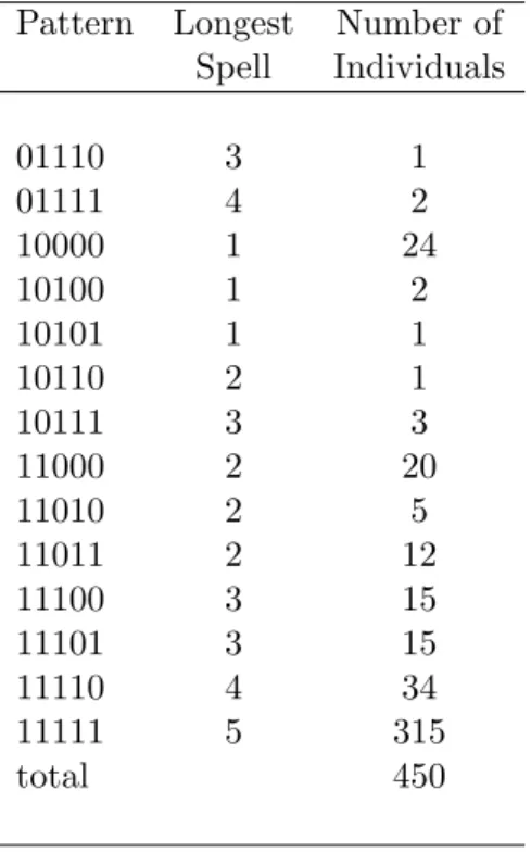
Table 3.2 details availability of data in each interview, where 10111, for example, indicates

that the participant missed the second interview. Note that I drop individuals aged 65 and

older due to retirement possibilities, those with ages 18-22 due to schooling possibilities and

one individual with no age information from the sample. Other individuals with missing

employment information were also dropped from the sample. Statistics reported from here

on are based on the 315 individuals with complete information for all interviews. These data

provide 1575 observations for analysis.

3.2 Health Variables and Scales

It is important to consider different issues in the measurement of mental illness. In the

mental health and labor literature, different strategies are used. One common approach is the

7

This was to resemble real work practice.

(26)

Table 3.2: Individual Participation Patterns over the 5 interviews

Pattern Longest Number of Spell Individuals

01110 3 1

01111 4 2

10000 1 24

10100 1 2

10101 1 1

10110 2 1

10111 3 3

11000 2 20

11010 2 5

11011 2 12

11100 3 15

11101 3 15

11110 4 34

11111 5 315

total 450

utilization-based approach (Frank and Gertler, 1991). With this method, the individuals are

asked if they have ever been treated for a mental disorder. If they answer yes, they are asked

to identify the diagnosed disorder. With another approach, individuals are asked varying

questions about their mental health status. They characterize each element as excellent,

good, fair or poor. A more recent approach utilizes symptoms and clinical algorithms to

determine diagnoses. Individuals respond to questionnaires that identify clinical symptoms.

These symptoms either directly indicate a mental health problem or are used in algorithms

to determine a diagnosis. Specifically, the diagnosis of major depressive disorder is based on

the patient’s self-reported experiences, behavior reported by relatives or friends, and a mental

status exam. There is no laboratory test for major depression.

The ARTIST trial consists of multiple scales that can be used to measure depression

and/or physical health: The Depression Diagnosis Interview Questions (DDI), The Hopkins

Symptom Checklist (HSCL), The Physical Symptoms Scale (PSS), The 9-item Patient Health

(27)

Short-Form Health Survey (SF-12).8 Each scale has specific benefits and shortcomings. There

is an SF-12 score for each interview. SF-36 is only used at baseline and in months 3 and 9. The

DDI questions are also only asked at baseline, and in months 3 and 9. Depression outcome

is assessed with two measures of core depressive symptoms, the HSCL-209 and SF-12 mental

health component scores. I use both the HSCL-20 mental health component score and SF-12

mental health component scores as measures of depression in this paper. Both are validated

measures of depression severity.

Depression severity is often defined as mild, moderate or severe. The levels are described

in terms of the extent to which the patient’s everyday life is affected: mild depression causes

only minor impairment of the patient’s work, social life and relationships with others. Major

depression, as defined in the DSM-IV, can be of mild severity. Moderate depression is

as-sociated with more obvious symptoms and is more likely to be noticeable to others. Severe

depression is characterized by affecting the patient so badly that he or she may be unable to

work or to relate socially to others. Full remission is defined as the absence of symptoms for

at least two months. For partial remission, full criteria for a major depressive episode are no

longer met, or there are no substantial symptoms, but two months have not yet passed. In

this study, I do not distinguish between full and partial remission.

HCSL-20

The Hopkins Symptom Checklist (HSCL) is a self report symptom inventory originally

comprised of 58 items representing symptoms commonly observed in outpatients. There

are five underlying symptom dimensions: somatization, obsessive-compulsive, interpersonal

sensitivity, anxiety and depression. The original 58-item symptom inventory expanded to

incorporate 32 additional items in four symptom dimensions: hostility, phobic anxiety,

para-noid ideation and psychoticism. The HSCL-20 is a 20-item modified subscale of the 90-item

Hopkins Symptom Checklist. The scores range from 0-4 with a higher score indicating a more

8

SF-36 and SF-12 are versions of the same scale.

9

The HSCL-20 is a 20-item modified subscale of the 90-item Hopkins Symptom Checklist. The 20-item scale includes the full 13-item depression subscale of these longer instruments plus 7 additional items that allow for an assessment of all Diagnostic and Statistical Manual, fourth edition (DSM-IV) items. Using these scales, an HSCL-20 mean score is calculated for each individual in each time period.

(28)

serious depressive episode. This continuous variable will be used in all estimations. To serve

as a frame of reference, the scores are divided into 4 categories, each representing a different

degree of depression.

HSCLt =

        

       

1 depression in remission: 0.00≤HSCLt<0.75

2 mild depression: 0.75≤HSCLt<1.50

3 moderate depression: 1.50≤HSCLt<2.00

4 severe depression: 2.00≤HSCLt≤4.00

(3.1)

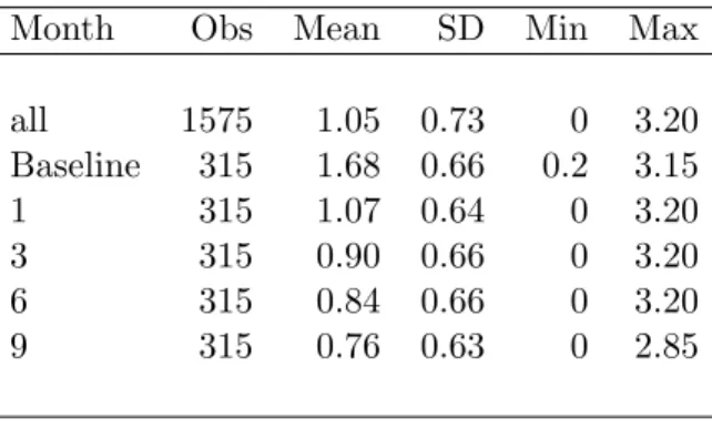
Table 3.3: Summary of Depression using HSCL-20 Score

Month Obs Mean SD Min Max

all 1575 1.05 0.73 0 3.20

Baseline 315 1.68 0.66 0.2 3.15

1 315 1.07 0.64 0 3.20

3 315 0.90 0.66 0 3.20

6 315 0.84 0.66 0 3.20

9 315 0.76 0.63 0 2.85

As seen in Table 3.3, the HSCL-20 mean measure continues to decrease throughout the

ARTIST trial, meaning that the patients’ general depression levels continuously improve. It

decreases at a decreasing rate until the last period with the largest improvement occurring in

the first period with a 36.30% change.

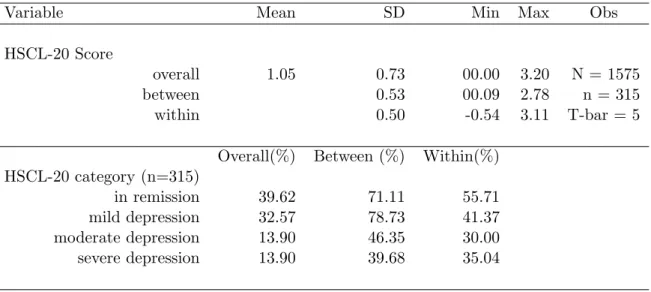
The trial follows individuals over time, and it is important to consider the breakdown of

the variation in the depression score into between-individual variation and within-individual

variation. I report similar statistics for the remainder of the outcome variables. Refer to

Table 3.4. Overall, 39.62% of the person-year observations are considered to be in remission

and 13.90% are categorized as having severe depression. Taking patients individually, 71.11%

of the individuals are in remission at some point, with 39.68% considered to be severely

depressed at least once; thus some individuals are characterized as having severe depressive

(29)

is considered to have major depression at least once, 35.04% of her observations fall into the

severe depression category. Similarly, if the patient is ever categorized to be in remission,

55.71% of her observations are considered to be in remission. If an individual’s depressive

status never varied over time in these data, the within individual variation percentages would

all be equal to 100. With a continuous variable, the mean and decomposed standard deviation

are reported. The standard deviation is decomposed into between and within components. If

the within standard deviation is equal to 0, all of the variation is between individuals. The

0.50 for the within variation confirms that there is variation within the individual.

Table 3.4: Variation in HSCL-20 Mental Health Variable

Variable Mean SD Min Max Obs

HSCL-20 Score

overall 1.05 0.73 00.00 3.20 N = 1575

between 0.53 00.09 2.78 n = 315

within 0.50 -0.54 3.11 T-bar = 5

Overall(%) Between (%) Within(%) HSCL-20 category (n=315)

in remission 39.62 71.11 55.71

mild depression 32.57 78.73 41.37

moderate depression 13.90 46.35 30.00

severe depression 13.90 39.68 35.04

SF-36 and SF-12

The 36-item Short-form Health Survey (SF-36) measures health-related quality of life

in eight domains, including physical functioning, social functioning, mental health, general

health perception, pain, vitality, and physical and emotional role functioning. Selected

mea-sures from the Medical Outcomes Study (MOS) are also used to assess social functioning,

concentration, positive well-being, hopefulness, sleep, and sexual function. Anxiety and

al-cohol disorder items are taken from the PHQ-9. Additionally, questionnaires were used to

evaluate quality of close relationships and disposition.

(30)

The 36-item short form was constructed to survey health status in the Medical Outcomes

Study (MOS), which was a part of the phone interviews at baseline, in month 3 and in

month 9. The SF-36 was designed for use in clinical practice and research, health policy

evaluations, and general population surveys. It includes one multi-item scale that assesses

aspects of both the individual’s physical and mental health: limitations in physical activities

because of health problems, limitations in social activities because of physical or emotional

problems, limitations in usual role activities because of physical health problems, bodily pain,

general mental health (psychological distress and well being), limitations in usual role activity

because of emotional problems, vitality (energy and fatigue), and general health perceptions.

Since this study is primarily concerned with questions surrounding mental health issues, I

will describe the questions that pertain to mental health. The 14 questions, out of 36 total

questions, affecting mental health fall into one of four scales (Vitality, Social Functioning,

Role- Emotional, Mental Health). The questions, scales and response alternatives that affect

the SF-36 score are found in Appendix A. The scores range from 0 to 100, with higher scores

indicating better mental health. As summarized in The SF-36 physical and mental health

summary scales: A user’s manual the best cut off for defining depression using the SF-36

mental health component score is at a score of 42.00 or below. This score minimizes the

possibility of either a false negative or a false positive. The false positive rate using this

SF-36 mental component scale cutpoint is 19.40% and the false negative rate is 26.30%.

The SF-12 was developed to be a much shorter, yet useful, alternative to the SF-36.

Only one to two questions are asked for each of the four scales (Vitality, Role Emotional,

Social Functioning, and Mental Health) rather than the three to four questions in the

SF-36. The choice between the 36-item or 12-item versions is largely practical and each has

advantages. The SF-12 is much shorter while reproducing the SF-36 summary scales very

well. It has the advantage of maximizing participant retention. The SF-36 profile has the

advantage of providing more information about the nature of differences in physical and

mental health outcomes. The SF-12 also uses a composite score of 42.0 as the cutoff score for

defining depression. The SF-12 interview is calculated in each month of the ARTIST trial.

(31)

In months 1 and 6, only twelve questions are asked so there is only a SF-12 score for each

individual interviewed in these months. The SF-12 scores will be used to divide the sample

into nondepressed and depressed individuals.

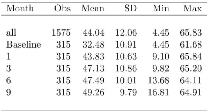
Table 3.5: Summary of Depression using SF-12 Score

Month Obs Mean SD Min Max

all 1575 44.04 12.06 4.45 65.83

Baseline 315 32.48 10.91 4.45 61.68

1 315 43.83 10.63 9.10 65.84

3 315 47.13 10.86 9.82 65.20

6 315 47.49 10.01 13.68 64.11

9 315 49.26 9.79 16.81 64.91

Similarly to when using the HSCL-20 component score, the SF-12 measure of mental

health continuously improves throughout the ARTIST trial as reported in Table 3.5, with a

higher score indicating better mental health. Patients experienced improvement each period,

with the largest improvement occurring in the first period with a 34.94% change. In Table 3.6,

it can be seen that there is within-individual variation for the SF-12 mental health measure

variation (SD=8.98).

Table 3.6: Variation in SF-12 Mental Health Variable

SF-12 Score

overall 44.04 12.06 4.45 65.83 N = 1575

between 8.06 15.26 61.78 n = 315

within 8.98 9.60 72.64 T-bar = 5

The SF-12 also includes questions related to physical health. The Physical Symptoms

Scale (PCS-12) is a scale consisting questions regarding the patient’s physical health. The

scores range from 0 to 100, with higher scores indicating better physical health. These

questions are asked at each interview. See Appendix B for the list of questions.

(32)

It can be assumed that any chronic condition will affect all decisions and outcomes in the

model. As a measure of medical comorbidity, I will use the Chronic Disease Score (CDS)

which is calculated at baseline for each patient. The CDS score increases with the number

of different chronic diseases as inferred from the subject’s medication profile. At baseline,

each patient is asked to list up to 14 prescription medications she is currently taking. With

these responses, the CDS score is calculated and used as a comorbidity index.10 Scores

have been shown to predict mortality and health care resource utilization after controlling

for demographics and previous resource utilization.11 As a measure of chronic depression,

at baseline, participants are asked if they had ever been treated for depression prior to the

ARTIST study. 34.60% of the individuals had experienced a depressive episode prior to the

ARTIST study. Baseline characteristics of these individuals are provided in Table 3.7.

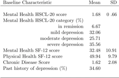
Table 3.7: Baseline Health Characteristics of Sample

Baseline Characteristic Mean SD

Mental Health HSCL-20 score 1.68 0 .66

Mental Health HSCL-20 category (%)

in remission 6.67 mild depression 32.06 moderate depression 25.71 severe depression 35.56

Mental Health SF-12 score 32.48 10.91

Physical Health SF-12 score 49.94 9.79

Chronic Disease Score 1.62 2.08

Past history of depression (%) 34.60

3.3 Labor Variables

The indirect costs related to depression can come in the form of presenteeism or

absen-teeism. The probability of being employed is also affected. This study uses three categories

of labor variables: participation variables (whether or not the individual is employed);

absen-10_{Specific medications are assigned to medication classes, which are then mapped to different chronic diseases.} 11

(33)

teeism variables (conditional on being employed, how often the worker is absent from work);

and presenteeism variables (conditional on employment, the worker’s productivity while at

work).

Work Limitations Questionnaire-Presenteeism and Absenteeism Variables

The Work Limitations Questionnaire (WLQ) labor variables are only used if the individual

answers yes to the following question: In the past two weeks did you work at anytime at a

job or business not counting work around the house?12

The objective of the WLQ was to develop a psychometrically sound questionnaire for

measuring the impact of chronic health problems and/or treatment on different job aspects of

employed workers. The WLQ is a self-reported instrument for measuring the degree to which

chronic health problems interfere with a workers’ ability to perform job roles with four

dis-tinct dimensions: handling time, physical, mental-interpersonal, and output demands. With

25 items, and a 2-week reporting period, the Work Limitations Questionnaire demonstrates

high reliability and validity. Unlike other questionnaires it addresses aspects of the job through

a demand-level methodology. In comparison to other questionnaires, the WLQ Output

De-mands scale, which I use to measure presenteeism, has superior performance for predicting

productivity. The Mental Interpersonal Demands and the SF-36 Role Limitation scales, which

are not used in this study, have moderate validity.13 A full listing of the questions can be

found in Appendix C.

Tables 3.8 and 3.9 report between-individual and within-individual variation for the labor

variables. In Table 3.8 it can be seen that there is within-individual variation in both the

employment probability measure and the ability to meet the required number of work hours.

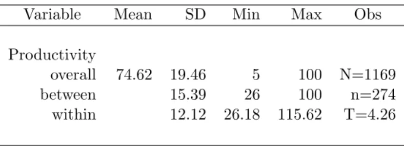
Table 3.9 reports means and standard deviations of the productivity measure for the overall

sample, between-individual and within-individual. The within statistics show the variation

of the ability to meet output demands within person around the global mean 74.62. The

within-individual SD shows that there is also within- individual variation in the productivity

12_{The wording of this question limits its use as an indicator of employment. An individual may still be}

employed if he/she has not worked in the last two weeks due to vacation, maternity leave, or an illness.

13_{For a full discussion of validity tests, see Lerner et al., 2002.}

(34)

measure.

Table 3.8: Variation in Labor Variables

Overall(%) Between (%) Within(%)

Employment Probability (n=315)

does work 74.22 86.98 85.33

does not work 25.78 46.98 54.86

Ability to Meet Required Work Hours (n=274)

All of the time 56.29 86.50 62.91

Most of the time 20.19 54.38 35.33

Some of the time 16.42 44.53 34.85

A slight bit of the time 6.07 19.34 30.74

None of the time 1.03 4.38 24.00

Table 3.9: Variation in Productivity Measure

Productivity

overall 74.62 19.46 5 100 N=1169

between 15.39 26 100 n=274

within 12.12 26.18 115.62 T=4.26

Table 3.10 presents descriptives statistics for each labor outcome by depressive state.

As expected the less depressed samples perform better for all labor variables. Employment

probabilities and depression levels show an inverse relationship, with 74.22% of the remission

sample being employed and only 67.00% of the sample categorized as having severe depression

working outside of the home. As depression levels decrease, the probability of working

con-tinuously increases. Less depressed workers are also better able to work the required number

of work hours. Again we see that the largest difference can be found between the depression

in remission sample and the mild depression group. The productivity measure also shows

(35)

productivity between the remission sample and those classified as having major depression is

larger than when comparing the sample’s employment probabilities and absenteeism.

Table 3.10: Summary of Labor Variables by HSCL-20 Mental Health Category

Variable n Mean SD Min Max

Employment Probability

full sample 1575 0.74 0.43 0 1

severe depression 219 0.67 0.47 0 1

moderate depression 219 0.72 0.44 0 1

mild depression 513 0.73 0.44 0 1

in remission 624 0.78 0.41 0 1

Ability to Meet Required Hours at Work

full sample 1169 4.24 1.00 1 5

mild depression 376 4.22 0.92 1 5

in remission 487 4.72 0.61 1 5

Productivity

full sample 1169 74.62 19.46 5 100

mild depression 376 73.11 16.25 5 100

in remission 487 86.60 11.73 35 100

3.4 Treatment Variables

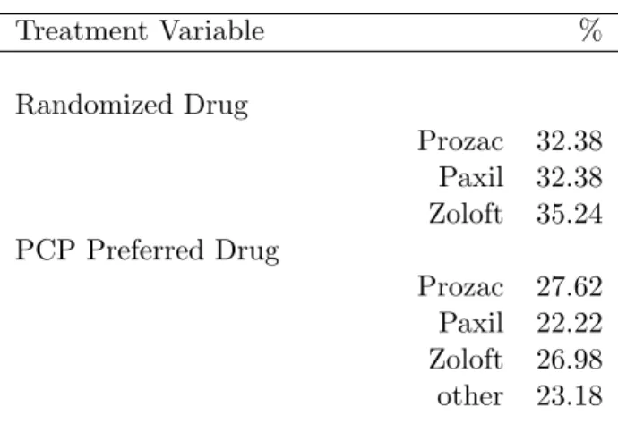
At baseline, a touch tone telephone procedure was used to randomly assign the patient to a

specific antidepressant: either Prozac, Zoloft or Paxil. A variable to indicate initial assignment

is created for each individual. Prior to randomization, the PCP is asked what antidepressant

he would prescribe in the absence of randomization. Responses included Celexa, Paxil, Prozac,

Wellbutrin, Zoloft or NA.14 These variables are summarized in Table 3.11.

A variable indicating if the same drug the PCP would have prescribed was randomized

14

N/A indicates that the PCP’s response was not Celexa, Paxil, Prozac, Wellbutrin or Zoloft.

(36)

to the patient at baseline is defined for each individual.15 Both patients and PCP’s were

aware of the baseline SSRI assignment. Decisions regarding treatment changes, including

SSRI type, dosage, and discontinuation were allowed and jointly made by the patient and

the PCP. At each interview, the individual is asked about her treatment decisions. She may

choose between continuing on the current drug, immediately switching to a new drug or

discontinuing use of the current drug without switching to an alternate medication. If she

chooses to change medication type, she is asked what type of SSRI she is currently taking.

At the next interview, she is asked about her treatment decisions with respect to the new

drug. 61% of the patients remain on the randomized drug throughout the trial. 20% of the

sample eventually stops the randomly assigned medication and does not immediately switch

to a new drug within the survey period, while 19% change SSRI medication and immediately

switch to a different SSRI at least once.

Table 3.11: Treatment Variables

Treatment Variable %

Randomized Drug

Prozac 32.38 Paxil 32.38 Zoloft 35.24 PCP Preferred Drug

Prozac 27.62 Paxil 22.22 Zoloft 26.98 other 23.18

Same Drug Randomized & Prescribed 33.33

15

(37)

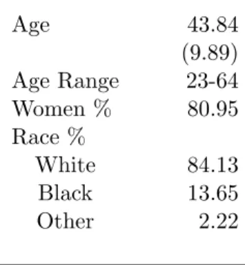
3.5 Exogenous Variables

Exogenous variables include the individual’s age, gender and race. Baseline characteristics

of the sample are found in Table 3.12. Additional time-varying information that may affect

outcomes exogenously are available from other data sources. Although participants report five

digit zip code information at each interview, Zip Code Tabulation Areas (ZCTAs) are used for

extracting Census 2000 and Current Population Study (CPS) information on a geographic

area from the reported zip code.16 Monthly state unemployment rates from the Current

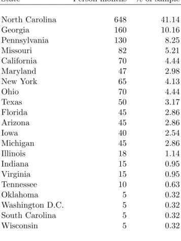
Population Study (CPS) are also used in the estimations. 21 states and Washington D.C.

are represented in the study. Table 3.13 describes the sample by state distribution. Current

local economic conditions facing the individual are likely to affect all employment decisions.

Therefore, they will be included in all labor equations.

Table 3.12: Summary of Baseline Individual Exogenous Characteristics

Baseline Characteristic

Age 43.84

(9.89)

Age Range 23-64

Women % 80.95

Race %

White 84.13

Black 13.65

Other 2.22

The month of the year is also included as a time-varying explanatory variable. The

calendar month of the year may affect both labor and health outcomes. Individuals may

experience more mental and physical health problems during the winter months. It is also

possible that labor outcomes may differ during specific times of the year. For example, a

worker may be more likely to take vacation during the summer months or during the winter

holiday time. Productivity may also be affected during specific times of the year depending

on the worker’s industry. Individuals enrolled in the study and completed baseline interviews

16

See Appendix E for discussion of ZCTAs.

(38)

Table 3.13: Represented States

State Person-months % of sample

North Carolina 648 41.14

Georgia 160 10.16

Pennsylvania 130 8.25

Missouri 82 5.21

California 70 4.44

Maryland 47 2.98

New York 65 4.13

Ohio 70 4.44

Texas 50 3.17

Florida 45 2.86

Arizona 45 2.86

Iowa 40 2.54

Michigan 45 2.86

Illinois 18 1.14

Indiana 15 0.95

Virginia 15 0.95

Tennessee 10 0.63

Oklahoma 5 0.32

Washington D.C. 5 0.32

South Carolina 5 0.32

(39)

during different months. On the interview date I create indicator variables=1 for each of the

twelve months.

(40)

Chapter 4 Theoretical Motivation

This section includes the theoretical background to the paper. In Section 5, I describe an

empirical approximation to the theoretical model that follows.

4.1 Overview of Decision Making Process

The individual enters a decision making periodtknowing her employment history, current

health status and her mental and physical health history. Future mental and physical health

are uncertain. With this knowledge, she decides whether or not to work in period t. By

accepting employment, she contracts for a certain number of hours of required work hours

(full time or part time). The required work hours are unobserved by the econometrician.

Conditional on working, the individual then decides the number of these required hours to

work and how productive to be for the duration of periodt. The individual must also decide

whether to continue her current medication, switch to another medication or discontinue

medication treatment entirely. The individual then realizes her health status at the end of

each period t. The per-period timing of decisions and realizations of health are depicted

below.

4.2 Decision Variables

Each period, individuals make optimal decisions with respect to employment and mental

(41)

beginning of t

et

employment decision

ot, at

productivity, attendance decisions Dt treatment decision

ht+1, bt+1

health production

beginning oft+ 1

St= (et−1, ot−1, at−1, Dt−1, ht, bt Xt,Zt)

-St+1 = (et, ot, at, Dt, ht+1, bt+1

Xt+1,Zt+1)

-Figure 4.1: Timing of per-period Employment and Treatment Decisions and Health Produc-tion

work outside of the home (et) where

et =

  

 

0 if individual does not work

1 if individual works.

If she decides to accept outside employment, she chooses her level of productivity for the

remainder of the period (ot) and attendance (at). The productivity measure (ot), a self

reported ability to meet output demands, takes the value 0 to 100, with 100 indicating

the highest productivity. With regard to absenteeism, the respondents answer the following

question: “Conditional on working, how much of the time during the past two weeks did your

physical health or emotional problems make it difficult for you to work the required number

of hours?” Attendance (at) takes on the values (with a higher score indicating less limitation):

at =

                      

1 All of the time

2 Most of the time

3 Some of the time

4 A slight bit of the time

5 None of the time

(42)

The individual makes the medication treatment decision (Dt). Treatment options include:

Dt =

     

    

0 if patient continues on the same drug

1 if patient immediately switches from the current drug to another drug

2 if patient stops current drug, does not immediately switch to new drug

When making decisions in period t, the individual may consider her employment status

(et−1), her productivity (ot−1), and her attendance at work (at−1) in the previous period.

She also considers her wage offer which depends on the worker’s employment history and past

performance. The wage offer is unobserved by the researcher.

Decisions may also be influenced by the individual’s health history including her treatment

decisions in the previous period (Dt−1), mental health state entering the current period (ht)1

where

ht =

        

       

1 if depression in remission

2 if mildly depressed

3 if moderately depressed

4 if severe depression

and physical health entering the current period (bt) where bt scores range from 0 to 100 with

higher scores indicating better physical health.

Current economic conditions such as median income by zipcode and monthly state

un-employment rates may also influence labor decisions and are denoted by the vectorZt. All

decisions are influenced by observed personal characteristics,Xt, including gender, race, and

age. The individual’s information, or state vector(St), entering period tis:

St= (et−1, ot−1, at−1, Dt−1, ht, bt, Zt, Xt). (4.1)

(43)

4.3 Health Production

An important part of this study is understanding how mental health evolves. The mental

health production function, or probability of a health transition from ht=h to ht+1=h0, is

modeled as

πhh_t₊₁0 = P r(ht+1=h0 |ht=h) ∀t

= exp{π0h0+π1h0ht+π2h0St+1} P4

h00=1exp{π0h 00₊_π

1h00ht+π2h00St+1}

. (4.2)

Particular components of St+1, namely (et, ot, at, Dt, bt+1, Xt+1), may influence depression.

Physical health (bt) also develops based on decisions and observed characteristics where

bt+1 =b(bt, ht, St+1). (4.3)

4.4 Optimization

An individual’s per period utility is a function of consumption (Ct), mental health status

(ht), labor choices (et,at,ot) and treatment decisions (Dt). LetJ equal the set of combinations

of the et, at, ot and Dt alternatives available to an individual. Each unique combination is

denoted j, j=1,2,3...J. Health status is assumed to have both direct effects (i.e., healthier

individuals derive more utility in all activities) and indirect effects (through its effect on

labor and treatment decisions) on utility. Treatment decisions affect utility through the

medication’s effects on physical health (side effects) and have productive effects on mental

health status. The individual’s per-period alternative-specific utility function is given by

U_tj =U(j, Ct, ht, bt, Xt, εjt) (4.4)

where εj_t represents alternate-specific and time-specific unobserved utility preferences and

consumption (Ct) is constrained by her budget. Sources of income include employment income

(44)

(Yt) if employed (et= 1) and unearned income (Wt) such that

Ct=et∗Yt+Wt. (4.5)

Employment income, Yt = Y(Xt, et−1, at−1, ot−1), is a function of personal characteristics,

and her employment history, days present at work and productivity in periodt−1. Ifet= 0,

consumption is constrained by unearned income. Treatment for depression is costless in these

data in pecuniary terms but may cause disutility through side effects, discomfort or stigma.

An individual is assumed to make decisions that will maximize her expected lifetime

utility. This includes the current utility of each alternative plus the discounted present value

of expected future utility where health and future utility shocks are uncertain. Her lifetime

value of each employment and treatment alternative is:

Vj(St, t) =Utj+

4 X

h0₌₁

πhh_t₊₁0Et

max

k∈J Vk(St+1, k t+1)|j

∀j ∀t (4.6)

where β is the discount factor. Since this research focuses on mental health and its effects

on labor market outcomes, physical health transitions are not modeled explicitly in the value

function. While physical health develops overtime, the value function assumes as written that

(45)

Chapter 5 Empirical Model

In measuring the effect of mental health on labor outcomes, many studies use the human

capital framework (Becker 1967, Grossman 1972) and assume people value good health for

both its direct effect on utility and its effect on human capital formulation. This paper focuses

on the relationship between depression and different labor market outcomes. Underlying the

analysis is the idea that for a group of depressed individuals, changes in depression levels lead

to changes in labor market outcomes. Additionally, treatment decisions affect health status.

In measuring the effects of depression on productivity and attendance for a group of initially

depressed individuals, there are multiple sources of bias that must be addressed in order to

obtain consistent estimates.

Two sources of endogeneity can lead to biased estimates of depression’s effect on labor

market outcomes. Structural endogeneity results from possible reverse causality. In this case,

the onset of depression may occur due to labor market outcomes. Statistical endogeneity

comes from potential unobserved factors causing depression that may also affect labor market

outcomes independent of depression. For example, unobserved personal characteristics, such

as excessive motivation or employment in high stress occupations may increase the risk of

depression and can lead to different labor outcomes. Including treatment decisions variables

explaining mental health transitions introduces additional potential bias in the measured

effect. Potential endogeneity results from permanent unobserved characteristics that affect

both the individual’s mental health status and treatment decisions.

(46)

workot and attendanceat, (Lit= [oit, ait]) if employed. The relationship is dynamic because

an individual’s labor outcomes depend on lagged endogenous variables. Let

eit =

  

 

1 if individual works in period t

0 if individual does not work in period t.

The work productivity (oit) and work attendance (ait) measures are only observed if the

individual works in period t (eit = 1). This dynamic model of labor outcomes includes a

lagged dependent variable as a regressor as follows:

Lit=δLi,t−1+αTi+βXit+εit ifeit= 1. (5.1)

An individual’s labor outcomeLit is related to time-invariant personal characteristics Ti1, a

vector of time-varying observables for the individual, Xit, and a disturbance term, εit. The

error component εit is decomposed as

εit=µi+νit (5.2)

where µi represents unobserved time invariant personal characteristics that will affect labor

outcomes (such as genetics) and νit accounts for random individual disturbances (such as

time-varying work demands). The vector of disturbances νit is assumed to be independent

and identically distributed (IID) IID(0, σ2_ν) and µi is distributed IID(0, σµ2). Substituting

equation (5.2) into equation (5.1),

Lit =δLi,t−1+αTi+βXit+µi+νit ifeit= 1. (5.3)

The binary choice selection model explaining whether an individual is working is described

by

e∗_it=ωΓit+ηi+ζit. (5.4)

1

Ti is not included in the theoretical model in the previous section. I separate this to clearly show the

(47)

where

eit =

  

 

1 ife∗_it>0

0 ife∗_it≤0

Γit is a vector of explanatory variables that may share elements with Xit, ηi is an

un-observable time-invariant individual-specific effect and ζit represents unobserved individual

time-specific disturbances. It is assumed that the error components in the two equations have

a joint normal distribution. This selection equation must be estimated jointly with the labor

outcomes in order to eliminate selection bias.

Dynamic panel bias and selection bias are additional sources of potential bias. Introducing

a lagged dependent variable complicates estimation when compared to a static model because

labor outcomes in past periods may also be correlated with unobserved permanent individual

heterogeneity,E(Li,t−1, µi)6= 0. Sample selection bias refers to problems where the dependent

variable is observed only for a restricted, nonrandom sample. In this case, the individuals

productivity in periodtis only observed if the individual is employed in that period. Similarly

to the productivity equation (the equation of interest), the employment equation (the selection

equation) may contain individual specific effects that are correlated with the explanatory

variables. To obtain consistent estimates, all potential sources of bias must be addressed.

In this study, the employment of an individual depends on unobserved time-invariant

char-acteristics of the individual such as motivation, ability or education level,E(eitµi)6= 0. These

characteristics are correlated with the unobserved individual effects from the productivity and

attendance equations.

If the potential sources of bias are due to time-invariant characteristics, a researcher can

time difference the data then use instrumental variables (IV) in a Generalized Method of

Moments (GMM) framework. The First-Differenced (FD) equation is:

(Lit−Li,t−1) =δ(Li,t−1−Li,t−2) +β(Xit−Xi,t−1) +νit−νi,t−1. (5.5)

(48)

This is equivalent to

∆Lit=δ∆Li,t−1+β∆Xit+ ∆νit. (5.6)

If the selection process is time constant, removing the fixed effect from productivity or

at-tendance equations eliminates any potential selection problem operating through µi. Now,

selection into employment is random when unrelated to the idiosyncratic errors νit, (i.e.,

E(eitνit) = 0). Since T = 5 and the entire panel covers 9 months, this is a realistic

assump-tion. For consistency, it is required that

E[∆νit|Xit, Xis, eit=eis = 1] = 0 ∀ s < t. (5.7)

First-differencing has the advantage that it eliminates the individual specific effects that are

correlated with both the explanatory variables in the labor equation and the selection

equa-tion. However, it does have an important weakness when an individual is not employed in

period t, eit 6= 1 ∀ t, since there is a gap in the panel.2 In these instances, there are no

productivity measures for these observations and withT = 5, many needed observations are

lost. A second transformation that will eliminate fixed effects without losing as many

obser-vations is called forward orthogonal deviations (FOD) (Arellano and Bover, 1995). Rather

than taking first-differences as in equation (5.5), it subtracts the average of all future available

observations of a variable. Therefore, despite the number of gaps, it can be computed for all

observations of Lit and explanatory variables except for t = 5. The orthogonal deviations

transform for any variablew is:

wi,t+1≡cit

wit−

1

Tit

X

s>t

wis

(5.8)

whereTit is the number of all future available observations. The scale factor to equalize the

variance of the transformed error, cit, equals

p

Tit/(Tit+ 1). With this transformation, the

disturbance term becomes

ν_i,t∗₊₁ ≡cit

νit−

1

Tit

X

s>t

νis

. (5.9)

2

A study of the dynamic relationships between depression, treatment, and work behavior