Emerging Science Journal
Vol. 3, No. 3, June, 2019
Position Control of a Flexible Joint via Explicit Model Predictive
Control: An Experimental Implementation
Massoud Hemmasian Ettefagh
a, Mahyar Naraghi
a*, Farzad Towhidkhah
ba Department of Mechanical Engineering, Amirkabir University of Technology, Tehran, Iran b Department of Biomedical Engineering, Amirkabir University of Technology, Tehran, Iran
Abstract
This paper experimentally controls a flexible joint via explicit model predictive control (Explicit MPC) method. The scheme divides the state space into different partitions, then solves the associated multi parametric optimization in off-line computations. The result stores in a look-up table to be used in on-line algorithm. First, the state space equations of the flexible joint are derived and linearized around the working point. Then, in order to meet the plant’s specifications, desired performance and the limitation of processor/memory, the constraints, weights, sampling time and prediction horizon are determined for the system. Finally, the algorithm is applied on the experimental plant. Numerous simulations, the result of the experiment and comparison with other methods confirmed that the method was able to control the vibrations of the constrained flexible joint.
Keywords:
Flexible Joint;
Explicit Model Predictive Control; Multi-Parametric Optimization; Discrete Linear Time Invariant System.
Article History:
Received: 10 October 2018
Accepted: 18 May 2019
1- Introduction
One of the important issues of industrial arms is backlash phenomenon in the joints and gearboxes and the associated nonlinear effects. One method of dealing with this problem is to use flexible joints. On the other hand, the flexibility produces some demerits, including the accuracy reduction in joint positioning and unwanted vibrations. To solve this problem and accurately position the robot arm, many control algorithms are proposed [1, 2].
Model predictive control uses a model of the plant to predict the future behavior of it through the prediction horizon time-span. The method employs the model to provide a control law that stabilize the system while the constraints are satisfied. At the beginning of the scheme, it was used exclusively to control stable and slow processes with large sampling times [3, 4]. Thanks to the state space approach and fast constrained optimization algorithms the method extended to different applications. Since then, many researches have done to further decrease the computations. Fast algorithms [5], tailored for the system with respect to its characteristics, parameterization of the input vector to decrease the number of decision variables [6, 7] are two successful of these attempts to decrease the computation times. Explicit model predictive control solves a multi parametric optimization problem and divide the state space into different partitions with respect to the active constraints. In addition to suits the benefits of model predictive control, advantages such as no need for an on-line optimization, easily implementation on industrial controllers with limited memory and processor and high reliability have made Explicit MPC a well-known method in industrial communities as well as in research groups.
This paper used Explicit MPC to experimentally control a flexible joint system. Weights, constraints, prediction horizon and sampling time selection as well as their effect on the system’s performance were studied here exhaustively. Step-by-step design procedure and the explanation of the implementation on the hardware device were other objects of
*CONTACT: [email protected]
DOI: http://dx.doi.org/10.28991/esj-2019-01177
this paper. The remainder of the paper is organized as follows. Section 2 is devoted to the derivation of the governing equations for the model and extracting constraints on the input and its incremental value and the state. In section 3, the theory of Explicit MPC is explained and the controller is designed for the system. Implementation of the designed controller and the evaluation of the performance in simulations and experiments are expressed in section 4. Finally, conclusion and final remarks are expressed in section 5.
2- Modeling of the Flexible Joint
Because MPC method uses a model to predict the future of the system, one needs to know the dynamics of the system to design the controller, in the first part of this section we drive the system’s equations of motion in state space. In the second part, input, rate of input and state constraints are determined for the system. To design a proper stabilizing controller, we have to have a relative knowledge of the values of the constraints because they represent practical restrictions of the system and violating them may lead to instability.
2-1- Dynamical Modeling of the System
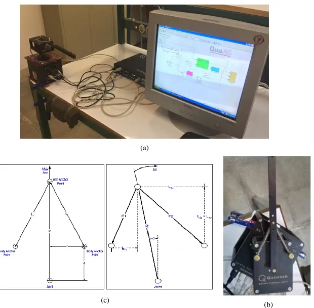
Figure 1 depicts the flexible joint system used in this paper. In this section we employ Euler-Lagrange equations to derive equations of motions of the system in state space.
According to Figure 1 the connection between the springs and the base is in such a way that we can substitute that with an equivalent torque. Then, this torque is used to determine the torsional stiffness of the joint. In other words, the applied torque M is 𝑀 = 𝐾𝑠(𝛼)𝛼 where α is the detection angle and 𝐾𝑠(𝛼) denotes the torsional stiffness which is also a function of the deflection angle.
(a)
(b) (c)
Figure 1. (a) Overview of the experimental setup, (b) the flexible joint and, (c) its schematic.
By assuming linear behavior of the springs, the rotational stiffness coefficient 𝐾𝑠(𝛼) is related to linear stiffness of the
(1)
𝐿1𝑥 = 𝑟 − 𝑅𝑠𝑖𝑛(𝛼), 𝐿1 𝑦= 𝑅 cos(𝛼) − 𝑑 , 𝐿1= √𝐿1𝑥2 + 𝐿21𝑦
𝐿2𝑥= 𝑟 + 𝑅𝑠𝑖𝑛(𝛼), 𝐿2 𝑦= 𝑅 cos(𝛼) − 𝑑, 𝐿2= √𝐿22𝑥+ 𝐿22𝑦
Which produce the following forces;
(2)
𝐹1= 𝐹1𝑥𝑖̂ + 𝐹1𝑦𝑗̂ = 𝐾𝐿(𝐿1− 𝐿) + 𝐹𝑟 , 𝐹1𝑥=
𝐹1𝐿1𝑥
𝐿1 , 𝐹1𝑦=
𝐹1𝐿1𝑦
𝐿1
𝐹2= 𝐹2𝑥𝑖̂ + 𝐹2𝑦𝑗̂ = 𝐾𝐿(𝐿2− 𝐿) + 𝐹𝑟 , 𝐹2𝑥=
𝐹2𝐿2𝑥
𝐿2 , 𝐹2𝑦=
𝐹2𝐿2𝑦
𝐿2 .
Where 𝐹𝑟 is tension force in springs when 𝛼 = 0, and 𝐾𝐿 is the stiffness coefficient of the linear springs. The resultant torque at the joint is;
(3)
𝑀 = 𝑅 × (𝐹𝑥𝑖̂ + 𝐹𝑦𝑗̂) = 𝑅 cos 𝛼 (𝐹2𝑥− 𝐹1𝑥) − 𝑅 sin 𝛼 (𝐹2𝑦+ 𝐹1𝑦).
The left hand side of (3) is equal to 𝑀 = 𝐾𝑠(𝛼)𝛼, so we can readily find the torsional stiffness of the joint. Since (3) is a nonlinear equation, the torsional stiffness is a nonlinear function of 𝛼. For small values of 𝛼 linearization around
𝛼 = 0 gives us
(4)
𝐾𝑠=
𝜕𝑀 𝜕𝛼|𝛼=0=
2𝑅 ((𝑅𝑟2𝐿 − 𝑑𝐷𝐿 + 𝑑𝐷3/2)𝑘 + (𝐷𝑑 − 𝑅𝑟2)𝐹 𝑟)
𝐷3/2 , 𝐷 = 𝑟2− (𝑅 − 𝑟)2.
The kinetic and potential energy and the equations of motion of the system are given as;
(5)
𝑈 =1 2𝐾𝑠𝛼2
𝑇 =1
2𝐽ℎ𝑢𝑏𝜃̇2+ 1
2𝐽𝑎𝑟𝑚(𝜃̇ + 𝛼̇)
2
(𝐽ℎ𝑢𝑏+ 𝐽𝑎𝑟𝑚)𝜃̈ + 𝐽𝑎𝑟𝑚𝛼̈ = 𝜏 − 𝐵𝑒𝑞𝜃̇
𝐽𝑎𝑟𝑚𝜃̈ + 𝐽𝑎𝑟𝑚𝛼̈ + 𝐾𝑠𝛼 = 0
Where 𝜃, 𝛼, 𝐽ℎ𝑢𝑏 and 𝐽𝑎𝑟𝑚 denote rotational angle of the hub, rotational angle of the arm, rotational inertia of the hub
at the joint and rotational inertia of the arm around the joint respectively. 𝐵𝑒𝑞 is the viscus damping coefficient between
the hub and the arm and 𝜏 is the applied torque from the actuator to the system. The relationship between 𝜏 and the controller output 𝑢 is given as [11]:
(6)
𝜏 =𝜂𝑚𝜂𝑔𝐾𝑡𝐾𝑔
𝑅𝑚 𝑢 −
𝜂𝑚𝜂𝑔𝐾𝑡𝐾𝑚𝐾𝑔2
𝑅𝑚 𝜃̇.
Numerical values of parameters and constants in (5) and (6) are 𝐽ℎ𝑢𝑏= 0.0021, 𝐽𝑎𝑟𝑚= 0.0019, 𝐾𝑠= 2.24, 𝐵𝑒𝑞 =
0.004, 𝐾𝑡= 𝐾𝑚= 0.0077, 𝐾𝑔= 70, 𝑅𝑚= 2.6, 𝜂𝑔= 0.9, 𝜂𝑚= 0.69 [11]. The state space vector is defined as 𝑥 =
[𝑥1= 𝜃, 𝑥2= 𝛼, 𝑥3= 𝜃̇, 𝑥4= 𝛼̇] 𝑇
; hence the linearized equations of motions in state space form are given as.
(7) [ 𝑥̇1 𝑥̇2 𝑥̇3 𝑥̇4 ] = [
0 0 1 0
0 0 0 1
0 982.8149 −1.7517 0
0 −2163.85 1.7518 0
] ⏟ 𝐴 [ 𝑥1 𝑥2 𝑥3 𝑥4 ] + [ 0 0 437.9316 −437.9316 ] ⏟ 𝐵 𝑢 ,
𝑦 = [𝜃
𝛼] = [1 0 0 0⏟ 0 1 0 0]
𝐶 [ 𝑥1 𝑥2 𝑥3 𝑥4
2.2. Modeling of the Constraints
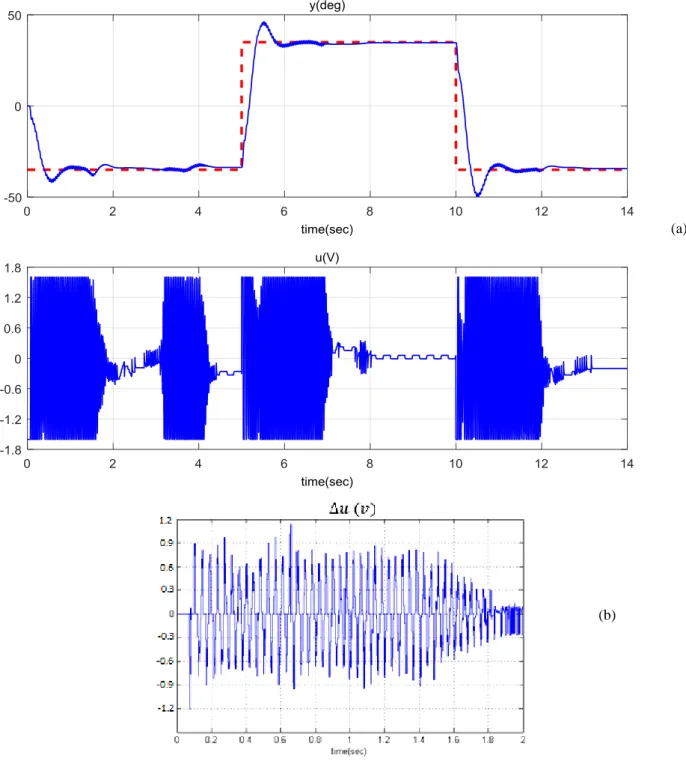
One of the main benefits of MPC is its ability to provide a control law that satisfies constraints. State and output constraints are usually defined for the system’s performance, so they are usually considered as soft constraints. Constraints on the input and rate of the input are related to actuators/systems characteristics and violation of them may leads to instability. Therefore, these constraints must be considered as hard constraints. In this section we employ some experiments to extract constraints on input, input rate and states of the system. In order to determine the constraint on the input and rate of the input, we used pole placement method to design a controller. Then, we set the poles of the closed-loop system to the far left of the 𝑗𝜔 axis till the closed-loop response of the system became unstable due to the uncertainties such as friction in gears, and un-modelled dynamics. This type of instability produced chattering behavior of the system under which the control signal was become saturated with the highest possible frequency. The saturation level was around 1.65 [𝑣]. Since the controller was working in the highest possible frequency, the constraint on rate could be obtained from Δ𝑢 = 𝑢𝑘− 𝑢𝑘−1. Figure 2 shows the valuse of constraints on the input and on the rate of the input. The mean value of the maximums of Δ𝑢, according to Figure 2 (b), is 0.9 [𝑣].
Figure 2. (a) input signal at its peak value, and (b) its rate 𝚫𝒖.
(b)
It is worthwhile to note that the required performance and physical restrictions of the system determine the state and output constraints. The required performance includes maximum velocity and error and the allowable value of the overshoot. These values are not very strict and can be modelled as soft constraints. However, there are another group of state/output constraints that deals with physical limitations of the structure, such as restriction of rotation of 𝛼 in Figure 1, and must be considered as hard constraints. According to our direct measurement and Figure 1, the constraints of 𝛼 and 𝜃 are determined as ±350, ±500 respectively. Therefore, system’s constraints are summarized as;
(8)
|𝑢| ≤ 1.65 [𝑣], |Δ𝑢| ≤ 1.2 [𝑣] , |𝜃| ≤ 0.87 [𝑟𝑎𝑑] , |𝛼| ≤ 0.61 [𝑟𝑎𝑑]
3. Designing of the Controller
In this section, we first briefly introduce the theory of Explicit MPC and then we employ the theory to design a controller for the system.
3.1. Explicit Model Predictive Controller
Consider the discrete linear time invariant system
(9)
𝑥(𝑖 + 1) = 𝐴𝑥(𝑖) + 𝐵𝑢(𝑖), 𝑦(𝑖) = 𝐶𝑥(𝑖), 𝑦min ≤ 𝑦(𝑖) ≤ 𝑦max , 𝑢min ≤ 𝑢(𝑖) ≤ 𝑢max ,
For this system, model predictive control solves the following optimization problem with respect to the initial condition𝑥(0) = 𝑥0.
( 10 )
𝐽∗(𝑥
0) = min 𝑢0,𝑢1,⋯,𝑢𝑁−1𝑥𝑁
𝑇𝑃𝑥
𝑁+ ∑ 𝑥𝑖𝑇𝑄𝑥𝑖+ 𝑢𝑖𝑇𝑅𝑢𝑖 𝑁−1
𝑖=0
𝑆𝑢𝑏𝑗𝑒𝑐𝑡 𝑡𝑜 𝑥𝑖+1= 𝐴𝑥𝑖+ 𝐵𝑢𝑖, 𝑖 = 0,1, ⋯ , 𝑁
𝑥0= 𝑥(0),
𝑦min ≤ 𝑦(𝑖) ≤ 𝑦max , 𝑖 = 0,1, ⋯ , 𝑁
𝑢min ≤ 𝑢(𝑖) ≤ 𝑢max , 𝑖 = 0,1, ⋯ , 𝑁 − 1
In which N denotes prediction horizon and Q, P, R are positive-definite matrices denoting weights on states, terminal states and the input. With some calculations, Equation 10 reduces to
( 11 )
𝐽∗(𝑥
0) = min𝑈 𝑈𝑇𝐻𝑈 + 𝑥0𝑇𝐹𝑈
𝑆𝑢𝑏𝑗𝑒𝑐𝑡 𝑡𝑜 𝐺𝑈 ≤ 𝑊 + 𝑆𝑥
Where U = [u0T, ⋯ , uN−1T ]T and matrices F, H, G, W, S are calculated from Equation 10- see [12] for the details.
The quadratic programming Equation 11 meets KKT conditions [13], so we can solve it as a multi-parametric
optimization and reduce the solution to [8];
( 12 )
𝑈∗(𝑥
0) = 𝐶1,𝑗𝑥0+ 𝐶2,𝑗= −𝐻−1(𝐹𝑥0+ 𝐺𝑎𝑐𝑡𝑇 𝜆𝑎𝑐𝑡),
𝜆𝑎𝑐𝑡 = −(𝐺𝑎𝑐𝑡𝐻−1𝐺𝑎𝑐𝑡𝑇 )−1(𝐺𝑎𝑐𝑡𝐻−1𝑆𝑎𝑐𝑡𝑥0+ 𝑊𝑎𝑐𝑡)
Where 𝑊𝑎𝑐𝑡, 𝐺𝑎𝑐𝑡, 𝑆𝑎𝑐𝑡 are rows of matrices 𝑊, 𝐺, 𝑆in [11] that determine the active constraints with respect to the given initial condition. It is shown in [8] that Equation 12 is a bounded piece-wise continuous function. Therefore, it divides the state space to limited number of partitions where each partition has its own exclusive control law. Next, the partitions and control laws are stored in a look-up table to be used on-line to control the plant [10].
3.2. Controller Design
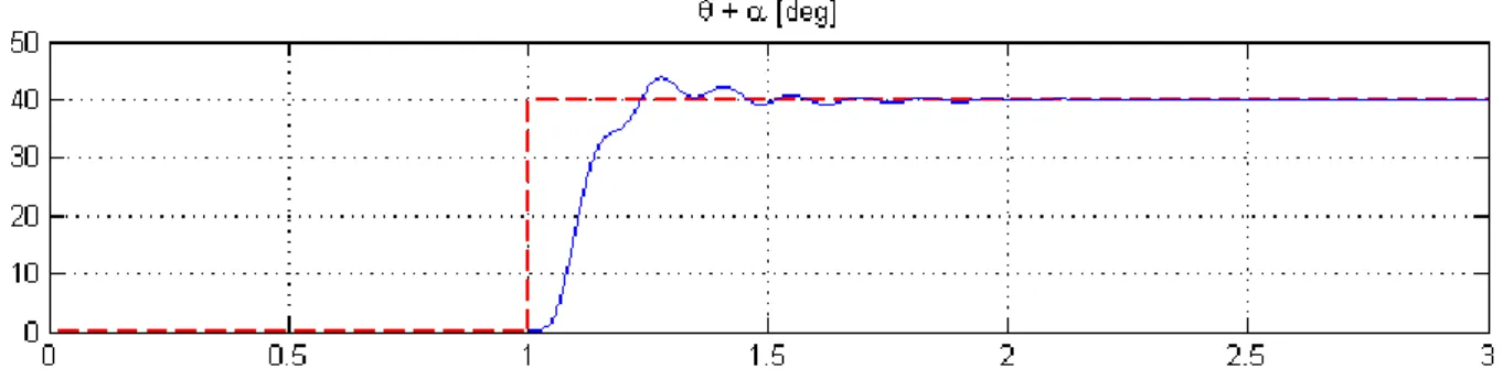
Based on the experimental setup’s characteristics we set the sampling time to Δ𝑡 = 0.002 = 2 𝑚𝑠 where is the smallest possible value of the data acquisition board. We start the simulations with 𝑄 = 𝐶𝑇𝐶, 𝑅 = 1 and then change Q as 𝑄 = 𝐶𝑇𝑄∗𝐶 to reach to the desired performance. Figure 3 shows the simulation result for 𝑄 = 𝐶𝑇𝐶, 𝑅 = 1 that has %10 overshoot and 1 sec setteling time. Flexibility of the joint is the main reason of overshoot.
Figure 3. Time response of the closed-loop system with DLQR controller. 𝑹 = 𝟏, 𝑸 = 𝒅𝒊𝒂𝒈([𝟏, 𝟏, 𝟎, 𝟎]).
As it is displayed in Figure 4, we can adjust the overshoot by changing the relative value of the elements of 𝑄 with eachother. Any increase in the first element, which is respect to 𝜃, decreases the raise time and increases the overshoot, control effort and transient error value of 𝛼. Figures 3 and 4 suggest us to choose 𝑄 and 𝑅 as
( 13 )
𝑄 = [
10 0 0 0
0 1 0 0
0 0 1 0
0 0 0 1
] , 𝑅 = 1
Figure 4. Time response of the closed-loop system with DLQR controller and different weights.
The terminal weight 𝑃 of Equation 10 is selected as the solution of Algebraic Ricaati Equation to imitate the infinite horizon behavior [14]. The value of 𝑃 is
( 14 )
𝑃 = 𝐴𝑇𝑃𝐴 + 𝑄 − 𝐴𝑇𝑃𝐵(𝐵𝑇𝑃𝐵 + 𝑅)−1𝐵𝑇𝑃𝐴.
In order to determine the appropriate 𝑁 and Δ 𝑡, we have to keep in mind that as sampling time decreases, the time for on-line calculations also decreases. To prepare the control effort in-time, the on-line calculations must be done during the time span of the sampling time, otherwise the system’s stability could not be assured. Therefore, the sampling time should be large enough for on-line calculations to be done. On the other hand, a large sampling time produces delay for the system that deteriorates the stability significantly. Another important parameter is the horizon. A large horizon is desirable in the sense that it increases stability; however, as the horizon increases the on-line computation load increases which means the sampling time has to increase too. To keep a balance between computation load, sampling time and horizon, we have to find the smallest horizon in which closed-loop stability is guaranteed in the simulations.
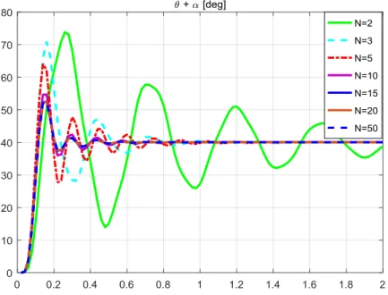
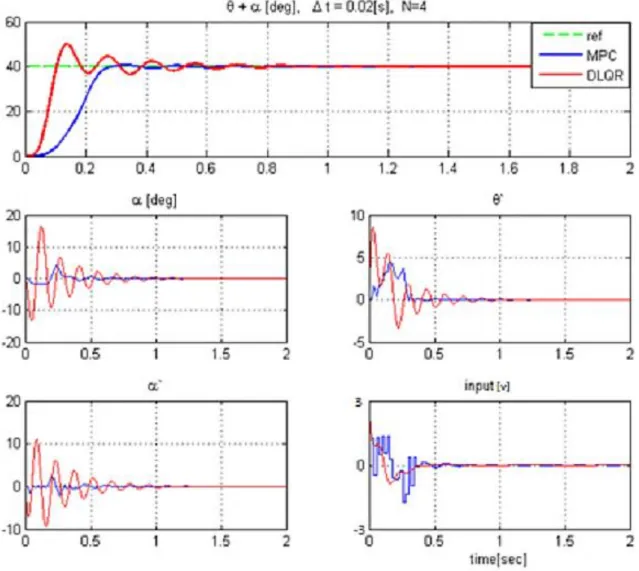
Figure 5 shows the sensitivity of the closed-loop solution to the prediction horizon. It shows that the quality of response is poor for 𝑁 = 1,2 and it improves significantly as 𝑁 increases (Note the difference between 𝑁 = 2 and 𝑁 =
Figure 5. Time response of the unconstrained system with different horizons and 𝚫𝒕 = 𝟐𝟎 𝒎𝒔.
Figure 6. effect of sampling time in system’s response.
The effects of applying constraints on the controller are shown in Figure 7. It depicts that the rise time in MPC is larger than the rise time in DLQR, but the settling time is the same for two controllers. In MPC solution, the selling time is equal to the rise time, while these values are considerably different in DLQR. Moreover, while the solution of DLQR produces overshoot, the MPC removes any overshoot from the closed-loop solution which is significantly important in industrial situations where the overshoot could be damaging.
Figure 7. Closed-loop performance after imposing constraints on input, rate of input and states.
4. Implementation of the Controller
In designing Explicit MPC, we should keep in mind that the main concern is to keep the on-line computations as small as possible. The on-line algorithm duty is to find the partition in which the measured initial condition is belong to, and then to apply the corresponding control law. Numerous research has shown that the most time-consuming part of the on-line algorithm is the determination of the partition [15, 16, 17]. Therefore, in order to keep the computation time minimum, we must decrease the number of partitions.
As it was mentioned before, the element is to keep the number of partitions as small as possible. We employed Yalmip [18] and mpt-toolbox [19] to extract Explicit MPC algorithm. In the first try, we designed the controller for 𝑁 =
5 that results to 4766 partitions. During the implementation, it was observed that the on-line search algorithm was not able to determine the partition of the given initial condition within the sampling time of 20 [𝑚𝑠]. Therefore, we used
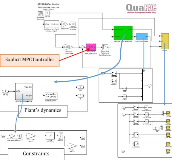
𝑁 = 4 for the prediction horizon which results in 1283 partitions. Then, we used the look-up table in Simulink to control the setup in Real Time Workshop. Figure 8 depicts an overview of the Simulink model where the explicit MPC is integrated through an embedded function. The joint rotations are measured with 1024-bit resolution encoders and
Figure 8. Simulation file for simulations and experiments.
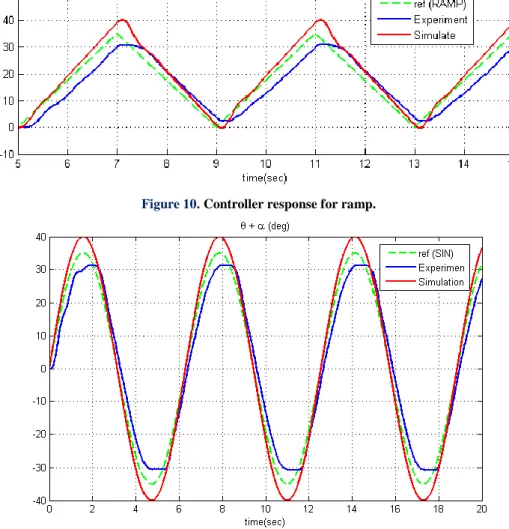
The response of the closed-loop system with explicit MPC controller for step, ramp and sine inputs are shown in Figures 9 to 11. In Figure 9, the constraints are set in such a way that the closed-loop solution is free from any overshoot. The result for step input is compared with the closed-loop result of DLQR controller. Both controller have the same settling time, but the rise time in DLQR is much less than the rise time in explicit MPC. Unlike DLQR, the closed-loop solution of explicit MPC shows no overshoot in the implementation. The discrepancy between the simulation and the implementation is a result of uncertainties, modeling inaccuracies and un-modelled dynamics. Figure 10 and 11 show the closed-loop response of simulation and implementation for ramp and sine inputs. Again, we can see some discrepancy between the simulations and the experiments, but the overall performance of the controller is satisfactory.
Figure 9. Controller response for step.
Plant’s dynamics
Figure 10. Controller response for ramp.
Figure 11. Controller response for sine.
5- Conclusion
In this article, the implementation of explicit model predictive control on a flexible joint was studied. The designing process such as weight selection, horizon selection and constraints values was explained step-by-step via a practical approach. The experiments showed the unwanted vibrations of the flexible joint can be reduced significantly with the explicit MPC approach. The ability to accommodate constraints is the main advantage of explicit MPC over DLQR. It was shown that the number of partitions is a major concern in this scheme and the designed should keep the it down as much as it can be.
6- Conflict of Interest
The authors declare no conflict of interest.
7- References
[1] Dwivedy, Santosha Kumar, and Peter Eberhard. “Dynamic Analysis of Flexible Manipulators, a Literature Review.” Mechanism and Machine Theory 41, no. 7 (July 2006): 749–777. doi:10.1016/j.mechmachtheory.2006.01.014.
[2] Shigang, Yue. “Redundant Robot Manipulators with Joint and Link flexibility—I. Dynamic Motion Planning for Minimum End Effector Deformation.” Mechanism and Machine Theory 33, no. 1–2 (January 1998): 103–113. doi:10.1016/s0094-114x(97)00028-1.
[3] Morari, Manfred, and Jay H. Lee. “Model Predictive Control: Past, Present and Future.” Computers & Chemical Engineering 23, no. 4–5 (May 1999): 667–682. doi:10.1016/s0098-1354(98)00301-9.
[4] Qin, S.Joe, and Thomas A. Badgwell. “A Survey of Industrial Model Predictive Control Technology.” Control Engineering Practice 11, no. 7 (July 2003): 733–764. doi:10.1016/s0967-0661(02)00186-7.
[6] Wang, Liuping. “Discrete Model Predictive Controller Design Using Laguerre Functions.” Journal of Process Control 14, no. 2 (March 2004): 131–142. doi:10.1016/s0959-1524(03)00028-3.
[7] Ettefagh, Massoud Hemmasian, Mahyar Naraghi, Farzad Towhidkhah, and Jose De Dona. “Model Predictive Control of Linear Time Varying Systems Using Laguerre Functions.” 2016 Australian Control Conference (AuCC) (November 2016). doi:10.1109/aucc.2016.7868014.
[8] Bemporad, Alberto, Manfred Morari, Vivek Dua, and Efstratios N. Pistikopoulos. “The Explicit Linear Quadratic Regulator for Constrained Systems.” Automatica 38, no. 1 (January 2002): 3–20. doi:10.1016/s0005-1098(01)00174-1.
[9] Hrovat, D., S. Di Cairano, H.E. Tseng, and I.V. Kolmanovsky. “The Development of Model Predictive Control in Automotive Industry: A Survey.” 2012 IEEE International Conference on Control Applications (October 2012). doi:10.1109/cca.2012.6402735.
[10] Alessio, Alessandro, and Alberto Bemporad. “A Survey on Explicit Model Predictive Control.” Lecture Notes in Control and Information Sciences (2009): 345–369. doi:10.1007/978-3-642-01094-1_29..
[11] Quanser Inc. (2011). SRV02 rotary servo base unit. User Manual.
[12] Ettefagh, Massoud Hemmasian, José De Doná, Mahyar Naraghi, and Farzad Towhidkhah. “Control of Constrained Linear-Time Varying Systems via Kautz Parametrization of Model Predictive Control Scheme.” Emerging Science Journal 1, no. 2 (September 19, 2017): 65. doi:10.28991/esj-2017-01117.
[13] Bazaraa, M. S., Sherali, H. D., & Shetty, C. M., Nonlinear programming: theory and algorithms. (2013), John Wiley & Sons. [14] Mayne, D.Q., J.B. Rawlings, C.V. Rao, and P.O.M. Scokaert. “Constrained Model Predictive Control: Stability and Optimality.”
Automatica 36, no. 6 (June 2000): 789–814. doi:10.1016/s0005-1098(99)00214-9.
[15] Baotić, Mato, Francesco Borrelli, Alberto Bemporad, and Manfred Morari. “Efficient On-Line Computation of Constrained Optimal Control.” SIAM Journal on Control and Optimization 47, no. 5 (January 2008): 2470–2489. doi:10.1137/060659314. [16] Geyer, Tobias, Fabio D. Torrisi, and Manfred Morari. “Optimal Complexity Reduction of Polyhedral Piecewise Affine
Systems.” Automatica 44, no. 7 (July 2008): 1728–1740. doi:10.1016/j.automatica.2007.11.027.
[17] Bemporad, A., and C. Filippi. “Suboptimal Explicit Receding Horizon Control via Approximate Multiparametric Quadratic Programming.” Journal of Optimization Theory and Applications 117, no. 1 (April 2003): 9–38. doi:10.1023/a:1023696221899. [18] Lofberg, J. “YALMIP : a Toolbox for Modeling and Optimization in MATLAB.” 2004 IEEE International Conference on
Robotics and Automation (IEEE Cat. No.04CH37508) (2004). doi:10.1109/cacsd.2004.1393890.