WAR, PEACE, AND TRANSPORTATION: USING COMPUTATIONAL MODELING TO EXPLORE THE EFFECT OF TRANSPORTATION
TECHNOLOGY ON WAR
Andrew Stephen Pennock
A thesis submitted to the faculty of the University of North Carolina at Chapel Hill in partial fulfillment of the requirements for the degree of
Masters of Arts in the Department of Political Science.
Chapel Hill 2007
ii
ABSTRACT
WAR, PEACE, AND TRANSPORTATION: Using Computational Modeling to Explore the Effect of Transportation Technology on War
(Under the direction of Thomas Oatley)
Studies investigating the effect of interdependence on conflict have produced contradictory empirical findings. Studies using datasets from the mid-19th century onward
DEDICATION
iv
ACKNOWLEDGEMENTS
This author owes a profound debt to several parties for their support of this thesis. Dr. Thomas Oatley encouraged this project from its beginning, patiently read many drafts, and made many useful suggestions. Dr. David Stotts introduced me to the world of object-oriented programming and spent many hours answering my many questions. He spent many more helping me to reconcile RepastJ with my vision of the project. Steven Cox proved a fast friend and helpful tutor on several occasions when the nuances of Java baffled me. Dr. George Rabinowitz was an enthusiastic supporter of the tact this thesis took. Daniel Serrano was essential in introducing me to SAS and a patient instructor.
Most of all, I owe Charity Lynn Pennock a profound debt for her patient review, numerous grammatical pointers, and love and support.
TABLE OF CONTENTS
LIST OF TABLES……….vii
LIST OF FIGURES………..viii
Chapter I. INTRODUCTION……….……….1
Expectations and Conflict.………....3
Trade, Guns and Butter………....4
Advances in Transportation Technology………..5
The Merits of Computational Modeling……….………...8
II. INTRODUCTION TO THE MODEL……….10
The Logic of IPE-Model………...………...….14
The Structure of a Round………..…….15
Assess ………....15
Offer Trade………...…….16
Set Defense………..………...17
Make War……….………..19
Reset Round………..……….21
III. GENERAL PATTERNS OF WARFARE………...………..24
IV. CAUSATION OF WAR IN THE SYSTEM………30
Dependent Variable……….31
vi
Descriptive Statistics of the Variables ……….………34
Results……….35
V. CONCLUSION………...………..39
VI. APPENDIX………...………40
LIST OF TABLES Table
1. Unit1 in Round One ………16
2. Decision Structure for Determining Defense Spending………18
3. Structure of a Round for Country C1 ………..22
4. Discerning between Causal Mechanisms……….………..31
5. Descriptive Statistics of Variables across All Observations………...……….34
6. Number of Times Significant Out of 50 Runs………..………35
7. Descriptive Parameter Estimates of Variables across All Observations.…………36
8. Number of Times Significant Out of 50 Runs………..………37
viii
LIST OF FIGURES Figure
1. Budget Constraints and Trade……….………...4
2. The Decision Whether or Not to Initiate War……….…….20
3. Sample Run………..25
4. Average Number of Countries at War across 50 Simulations………26
5. Median Number of Countries at War across 50 Simulations……….27
6. Minimum and Maximum Number of Countries at War across 50 Simulations……….…….…….…….…….………...28
Chapter 1: Introduction
“These more dynamic models of how international trade and domestic politics interact are an important area of research. They may tell us a good deal about what the rush to free trade, if sustained, may mean for the future. Will the global liberalization process bring increasing pressures for more openness and for democracy? Or will it undermine itself and breed demands for closure and a backlash against governments and the international
institutions that support openness? Will openness produce a peaceful international system or one prone to increasing political conflict? The
answers to these questions will in turn tell us much about the future direction of trade policy globally.” (Milner, 1999)
Does economic interdependence affect conflict between nations? Existing research on interdependence and conflict offers an incomplete set of theories and conflicting
evidence. Liberal scholars argue that Kant’s initial intuition is correct: increased
interdependence lessens the likelihood of conflict. (Kant & Smith, 1903) Mansfield and Pollins (Mansfield & Pollins, 2003) outline three reasons for this effect: that trade is a substitute for gains otherwise accrued through war, (Rosecrance, 1986) that trade creates better communication between dyads of trading partners resulting in greater ability to negotiate peace (Stein, 1993), and that trade creates interest groups who lobby for peace so they can continue trading.
2
independent trading partner. The less dependent partner, through the threat of cutting trade, can gain concessions from its weaker trading partner. It is argued that this mechanism of manipulation is why we should be skeptical of a peaceful future brought about through increasing levels of trade.
In addition to these conflicting hypothesized causal pathways, studies have presented conflicting evidence about interdependence and war.(McMillian, 1997) When data from the later part of the 19thcentury onwards is used, trade is statistically linked to a greater
likelihood of peace.(Domke, 1988; Gasiorowski & Polachek, 1982; Mansfield, 1994; Oneal, Oneal, Maoz, & Russett, 1996; Oneal & Russett, 1997; Oneal & Russett, 1999a; Oneal & Russett, 1999b; Polacheck, 1980) Several scholars have focused on the seventeenth and eighteenth centuries and concluded that increased interdependence creates conflict.(Holsti, 1991; Levy & Ali, 1998; Levy, 1999) Still other authors find that when time is controlled for, then the effect of interdependence on peace is no longer significant. (Beck, Katz, & Tucker, 1998)
I theorize that understanding the role of transportation technology in the
international system can help explain these disparate findings. Other international relations scholars have theorized that transportation technology is a key component of understanding international change.1 Robert Gilpin (Gilpin, 1981) and Lars-Erik Cederman(L. Cederman,
2003) view technological change as affecting the reach of nations and therefore their ability to make war against their peers. However, neither explores the connection between trade, transportation technology and warfare. Do different levels of transportation technology impact the probability of nations going to war?
1Scholars from other subfields have also studied the effects of changing transportation technology on political
Expectations and Conflict
Nations, and more particularly their selectorates, have expectations of welfare.2
When these expectations are not met, leaders must find a new source of goods with which to satisfy the selectorate. If new trading partners can be found, welfare levels can be
maintained without resorting to war. If they cannot, then war becomes an option. I posit that governments decide to fight wars because they face a guns-butter tradeoff (Viner, 1948) which is inherently contingent on stable international trade relationships. Chourci and North describe a dynamic similar to this one in their discussion of "lateral pressure.” (Choucri & North, 1975) Although Choucri and North argue that lateral pressure results from internal growth and an increasing demand for resources, the point is the same: changes which reduce per capita domestic consumption put pressure on governments to take international action. I suggest that lateral pressure can be caused by changes in trade configurations brought on by technological change. Unless replacements can be found, if a country loses trade partners when trade configurations change then per capita domestic consumption will decrease and domestic welfare losses will occur. When this pressure reaches a given threshold it can cause decision-makers in a country to displace the welfare losses either through taking from other countries through war or by displacing consumption of specific groups inside their own country. Exploring how consumption is redistributed internally would be an interesting endeavor, but is outside of the scope of this project.
Trade, Guns and Butter
Every country has a finite number of resources available to consume. In the classical “guns-butter” tradeoff, countries must decide whether they will spend their resources on
4
domestic consumption or on building a military. Ideally, countries would spend at the x-intercept in the figure below, spending all of their resources on butter. But as the threat of war is ever present in the international system, countries also spend a portion of their resources to maintain a national military.
Under autarky a country’s spending on either guns or butter is constrained by how many resources it has available domestically. When countries begin to trade, they begin to receive gains from trade. (Krugman & Obstfeld, 2003; Oatley, 2006) These gains shift the production possibility frontier outward. Therefore, a country may now spend more on guns, butter or both.
Figure One: Guns, Butter and Trade
trading partner due to a shift of demand from their goods to other countries’ goods; one country’s decision to trade with another partner; or if a trading partner has been destroyed through conflict. When a partner in trade disappears, domestic consumption necessarily falls unless a replacement partner can be found.
Advances in Transportation Technology
In order to understand exactly how changes in transportation technology affects the probability of warfare occurring in a system, it is important to understand how
transportation technology has evolved overtime. Instead of gradually and continuously improving, the world has become more interconnected in fits and starts. (Hugill, 1993) From the 1500s, transportation technology has increased in a stepwise fashion; a new technology is introduced and then a period of time passes before another increase in technology appears. While levels of trade have fluctuated over time, the technologies underlying these changes have not regressed. The Pandora's Boxes of the sailing ship, the airplane, and containerized cargo ship have irrevocably increased the physical accessibility of nations to each other, increasing the possibilities for both commerce and warfare. As
transportation technology has increased the world has become more interconnected.3(Frieden, 2006)
When transportation technology increases, the number of partners each country can trade with increases. If they can find a more desirable partner after an increase in
transportation technology, they will leave current trading relationships and enter into new trading relationships. If a country loses a trading relationship, then it must either find a new
3It is likely that this process of increasing trade is not yet finished. The Internet can usefully be thought of as
6
partner or consume less than it did before the technological change occurred. When a new trading partner is found, the consumption loss, which would have occurred from a cessation of trade, is prevented. Finding new trading partners enables countries that have lost trade partners to continue trading and consuming.4
When trading partners shift, economic winners and losers are produced, not through explicit manipulation as the Realist would argue, but through the trading constituencies seeking their own best interests. This shift causes a decrease in consumption for those countries that have had trade shift away from them. Their production possibility frontier changes accordingly and the frontier shrinks back to pre-trade levels. (Figure One) Countries suffer as their gains from trade disappear (and rather suddenly).
This is a different conception of the question of “why war?” than either the liberals or the realists would present. Having a different answer to “why war?” allows us to offer a unique explanation to the adjunct question of “how does interdependence affect war?” The outcomes of shifts in trading relationships are not constant over time. Shifts in trading relationships interact with the relative number of trading partners to create broad patterns of war in the international system. The model presented below tests the theory that early in the development of a trading system, shifts in trade between nations results in high levels of warfare. This is due to the absence of alternate trading partners who can absorb the
economic blow of the abandonment of trade relations. Later, when the trading system becomes more integrated, the shock of losing trading partners is less likely to result in warfare. A computational model founded on the micro-motivation of maintaining current
4One of the basic assumptions underlying this pattern is that the system contains independent political units
consumption levels, either through trade or through war, can be used to examine whether or not transportation technology has an effect on the probability of countries instigating wars.
If the number and makeup of trading partners increases over time, we can explain the changing frequency of warfare by constructing a dynamic theory of the effects of trade over time. When the computational model described in the following section is run, the results of these shifts in trade are dynamic across time. When the number of trading partners is relatively small then these shifts in trading relationships produce frequent wars, but as time goes by the likelihood that a shift in trade results in war is reduced. As countries have more available trading partners the negative effects of the shift in trade from one partner to another are reduced. The market appears to be providing the security that a government would be providing to economic losers in a domestic setting. Without the presence of a political organization who is able to ameliorate the effects, the model indicates that the larger the number of trading partners the more likely peace is.
Other theories exploring the interplay of trade and conflict do not incorporate the idea that trading partners shift over time and that this shift can cause losses that societies are willing to go to war to recoup. Increases in transportation technology can enable a country to leave a current trading partner for a more desirable one. The country that loses a trading partner can either consume less, find a new partner, or go to war. The likelihood of finding a replacement trading partner is also a function of transportation technology, because increases in transportation technology also increase the number of partners available for trade.
8
technology, the chances of finding a replacement partner increase. The question is how to investigate this hypothesis.
The Merits of Computational Modeling
While it is possible to explore this theory using a time-series analysis, an alternate method of exploration is the use of computational modeling. Computational modeling as a method of inquiry can be quite different than that of most formal social science. Agent-based modeling provides international relations researchers with a useful and unique tool with which to investigate theories.
Much of international relations research seeks to find evidence in support of theory by using historical data. This limits the field’s ability to draw conclusions when there is only one set of data from the last 100 years in which to test systemic theories. This places international relations scholars in a methodological pickle. Increasing the number of
observations by decreasing the size of the time period can somewhat ameliorate the problem by providing more data points. Case studies provide another means for the international relations scholar to test theories, but are limited in its ability to draw broad conclusions. Agent-based modeling provides one way around the n=1 problem of modern systemic history.
can trace the paths to equilibria. Yet the great strength of computational models is their ability to uncover dynamic patterns.” (pg. 8)
Chapter 2: Introduction to the Model
Computational modeling was first applied to the field of international relations in the 1970s and 1980s. (Bremer & Mihalka, 1977; Stoll, 1987) Most recently, and most
prominently, Lars-Erik Cederman and his coauthors have produced a series of agent-based models with a distinctive set of characteristics. First, their models attempt to model war in the international system. They have produced models with a number of different variations on this theme including emergent borders(L. Cederman, 1997) and the inclusion of
democratic regimes(L. Cederman, 2001; L. Cederman, 2002). Both models place the actors in an environment conceptualized from a Realist framework. Second, Cederman, et al’s models rely on a grid system as the fundamental analogy for conceptualizing the
international system. In a grid system, countries can inhabit multiple cells in the grid but are only allowed to interact with those countries to which they are adjacent. Since Cederman published Emergent Actors in World Politics in 1997 his models have become increasingly complex but have remained rooted in the grid system. (L. Cederman, 1997) Other agent-based modelers have also employed the grid system in order to model various political phenomena. (Bhavnani, 2003; J. M. Epstein, Axtell, & 2050 Project, 1996; Lustick, 2000; Lustick, Miodownik, & Eidelson, 2004) The final basic assumption of Cederman's family of models is that war is a random, probabilistic event that, once triggered, results in nations fighting until one destroys the other.
focused their models exclusively on the security side of the field and ignored the possible interactions with the field of international political economy. Only one article, to my knowledge, has attempted to model trade and war together. Bearce and Fisher investigate the relationship of war, trade and polarity.(Bearce & Fisher, 2002) While they embrace the importance of geographical representation as other models have, they challenge the assumptions of previous models by choosing to model war as an endogenous process. Bearce and Fisher create a model in which changing transportation technology influences trade and war. Bearce and Fisher complicate their model by including the possibility for incomplete information and bargaining in an attempt to implement the ideas of
Fearon(Fearon, 1995) and Morrow(Morrow, 1989).
Like Bearce and Fisher, the model presented here challenges several of Cederman’s assumptions, but does so without unduly complicating the model with game theoretic concepts. I challenge Cederman’s models because they neglect trade as a part of the international system, do not have an endogenous reason for why war occurs, and do not represent the international system as a network, but as a grid. As Waltz correctly argues, there is much to be said for creating parsimonious models.(Waltz, 1979) Therefore, what is to be gained from challenging the construction of Cederman's models and creating a less parsimonious model of the world? First, while many international issues are best
conceptualized as security problems, trade certainly plays a role in international
politics.(Keohane & Nye, 2001) Fully half the field of international relations is neglected when trade considerations are not accounted for. Second, trade and war may be interrelated in important ways as hypothesized earlier.
Once trade is added as a dynamic in the model, it is necessary to use a
12
country. Using a grid system captures the idea that some of the world functions in two-dimensional space. Rather than conceptualizing the world as a grid, this model
conceptualizes the world as a network. In this network each country is a given distance from every other country and is able to fully interact with a country when transportation
technology allows them to be connected. In the language of formal mathematics, networks consist of nodes and edges which connect one node to another. In this model, nodes are used to represent countries and edges are created between each and every country in the set of 200 countries. In order to model distance between any two countries, each edge
connecting them is assigned a random value between zero and one. By connecting the nodes in this fashion the idea of two-dimensional space is left behind. The distance between any three countries is not a product of a geometric relationship. The distance between country one and country two and country two and country three does not condition in any way the distance between country one and country three. This conceptualization can seem an awkward bending of spatial reality but it captures the reality of the world that trade volumes are not always a function of adjacent borders. The advantage of using this network framework is that, unlike a grid, it captures the reality that at high levels of transportation technology every country is equally connected every other country.
It is worth noting that this model is also a systems model. For example, when a country looses a trading partner and is unable to find another partner, it can make war with any country that it is close enough to trade with not just the lost partner. That is, changes in the relationship between two trading partners can have an effect on third parties. In this respect the model captures the systemic effects of shifts in trade.5
5Other scholars have studied systems and system models (Jervis, 1997; Penubarti & Ward, 2000; Polachek,
To investigate the systemic effects of shifts in trade, I create a model that meets Epstein’s five criteria for generative social science. (J. M. Epstein, 1999) In order to qualify as generative social science, a model must have the following. First, the units involved must be heterogeneous. Second, they must be autonomous. Third, they must engage in an explicit space. Fourth, their interactions must be local. Fifth, they must be boundedly rational. If each of these conditions holds then the generative social scientist can answer the generativist's question which is "how could the decentralized local interactions of
heterogeneous autonomous agents generate the given regularity?" In this case, the given regularity is the relationship between interdependence and war.
The model presented here falls squarely within this framework. The model begins with 200 agents engaging each other under the same set of rules. The agents differ from each other only in that they are randomly endowed with different abilities to produce two goods at the beginning of each simulation. Each agent makes autonomous decisions each round during the simulation based on the amount of domestic consumption, or “butter,” consumed each round. The amount of butter consumed is defined as the total GDP of a country minus the amount spent on their military; the classic guns versus butter tradeoff. (Viner, 1948) All agents are boundedly rational and make decisions about whether or not to engage in war or trade based on relatively simple decision rules.
This paper uses a computational model dubbed IPE-Model (so named for its contrast to previous models) to explore if patterns of warfare can be explained by increases in transportation technology. IPE-Model is a Java program implemented using the
programming package RepastJ.6 For the purposes of the discussion here, IPE-Model can be
seen as a master program which orchestrates a fixed number of other programs which
14
represent countries. IPE-Model then coordinates each of the units, giving each the chance to make individual decisions about trading and making war upon other countries. IPE-Model records key information about each unit in each period in a database. It also records statistics about the system as a whole at each period.
The Logic of IPE-Model
The main program, IPE-Model, is structured as follows. At the beginning of each run IPE-Model creates a world of 200 units which abstractly represent countries. Each unit has the exact same logical structure and therefore each unit responds to the same scenario in exactly the same fashion.
At the beginning of each simulation each unit is endowed with a randomly determined amount of two complimentary goods, A and B. Each unit is given a random distance between zero and one from every other unit. These distances are distributed using a random number generator (0,1) with a uniform distribution.
In each round a series of actions are executed by every unit in the system.7
IPE-Model asks all 200 countries in sequence to perform each action before moving to the next action. For the first action, assess, each unit is asked to conduct the same series of
calculations. After every unit in the system has executed this action then the next action is called. After every unit has preformed each and every action then an action called resetRound is executed which ends the round. When resetRound is executed, information is gathered, displayed graphically, and written to a database for analysis.
During a run the only value of a unit variable which is exogenously changed by IPE-Model is the range of vision which each unit has. This variable, internally referred to as
technology, represents the transportation technology available to countries in the system at
each time period. At the beginning of a run each unit can see only other units that are within its original range of vision, .05 out of a possible 1.0. Since distribution of how far away every unit is from every other unit is set in a random and uniform fashion the number of units visible to any one unit at the beginning of a run with 200 units is probabilistically eight. Every fifty rounds, the range of visibility is increased by an increment of .05. This results in an increasing number of potential trading and fighting partners until round 950 when every unit can interact with every other unit. This increase in vision represents technological change. Each run of the simulation consists of 1,000 rounds.
The Structure of a Round
During each round, every unit in the model is asked to do each of the following actions in the following order. Each action is executed for each unit before moving onto the next one. Table Two, presented at the end of this section, summarizes what happens to a country in each round. These actions are described in detail below.
Assess
At the beginning of each round it is important that each unit know two things about itself: (1) how much excess of either good A or good B it has to trade and (2) what units it is able to interact with this round. The method assess is called to ask each unit to calculate these two quantities.
16
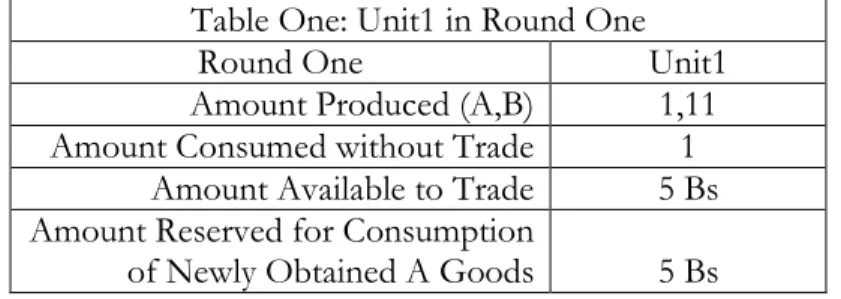
each round is a function of the amount of A and B produced during the previous round. A and B are defined to be complimentary goods. The total amount that each unit is able to consume is whichever good, A or B, the unit has the least of. Each unit places one half of the extra unconsumed amount in a “tradable” variable and keeps the other half to use when the complimentary good is traded for. For example, if Unit1 has one A and 11 Bs (1,11) it consumes 1 AB pair. It then takes the remaining 10 Bs, keeps half (five), and puts the other half (five) on the market in hopes of trading them for five A’s. These five Bs are stored in a variable called “tradable.”
Table One: Unit1 in Round One
Round One Unit1
Amount Produced (A,B) 1,11 Amount Consumed without Trade 1
Amount Available to Trade 5 Bs Amount Reserved for Consumption
of Newly Obtained A Goods 5 Bs
The second action taken by each unit in assess is to systematically look at all of the other units in the system and check to see if they are available to trade with or make war against this round. If the distance from Unit1 to Unit2 is less than the maximum distance that the units can see given the level of transportation technology in that round, then they are able to both trade and make war with each other as their decision trees dictate. Unit1 and Unit2 are “visible” to each other. If the distance between them is greater than the maximum distance then they are not visible to each other and they will not interact this round.
offerTrade
amount of excess A or B it had to offer and stored that amount in a variable called “tradable.” Each unit takes this excess and offers it to the first unit on its list. If the other unit has an excess of the opposite good, a trade is negotiated and the amount of A and B consumed by both units increase.8Once a trade is executed, each unit determines if it has
more to trade. If it does, the unit continues offering trades to the other visible units in the order which they appear on its list. Each unit’s list has a unique starting point. Trades are offered until the unit either runs out of goods to trade or partners to ask.
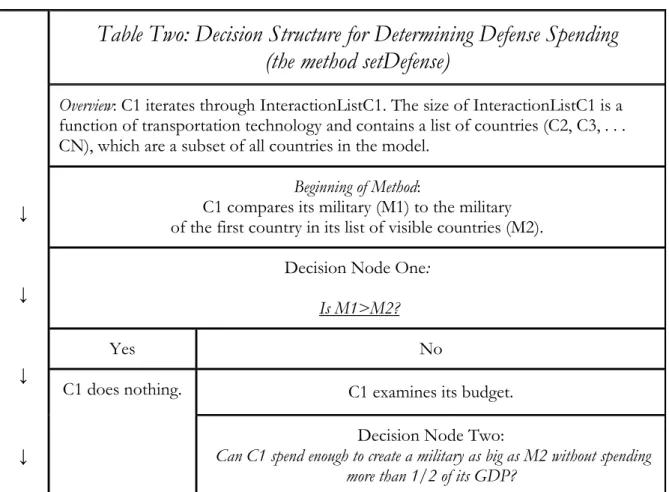
setDefense
In setDefense, each unit compares its own defenses to that of the other units that are visible to it. The first unit called in the first round (Unit1) looks at its first visible neighbor (Unit2) and asks it for its army size. In the first round Unit2 does not yet have an army. In the opening round, Unit2 decides to build an army and determines the size of that army by multiplying the amount it consumed after trading by a ratio (.2) dubbed
“initialDefenseRatio.” Unit2 then tells Unit1 the size of the army it has created.
When Unit1 receives this information, it then makes a series of decisions to decide what size army it should have. Each unit will spend up to one half of its total consumption on building an army. If the army of Unit2 is greater than one-half of Unit1’s post-trade consumption then Unit1 will build an army that is one half of its own consumption. If the army of Unit2 is smaller than one half of Unit1’s consumption, then Unit1 sets its army to the size of Unit2’s.
8The unit receiving the offer uses the method acceptOffer to if the offer should be accepted and how much of
18
Unit1 then goes on to examine each of the other units that are visible to it. When it encounters an army that is larger than its current army, it follows the same decision process detailed above. When this process is finished it subtracts the size of the army it has created this round from the amount it consumed after it finished trading. The remainder is how much “butter” it has been able to consume this round.
Domestic Consumption = Butter + Guns
This formula conceptualizes the inherent tradeoff countries must make in choosing between domestic consumption and military spending.(Viner, 1948) Table Two details the set of decisions described above.
Table Two: Decision Structure for Determining Defense Spending
(the method setDefense)
Overview: C1 iterates through InteractionListC1. The size of InteractionListC1 is a function of transportation technology and contains a list of countries (C2, C3, . . . CN), which are a subset of all countries in the model.
Beginning of Method:
C1 compares its military (M1) to the military of the first country in its list of visible countries (M2).
Decision Node One: Is M1>M2?
Yes No
C1 examines its budget.
P
P
P
P
C1 does nothing.
Decision Node Two:
Yes No
P
C1 spends enough to set
M1 = M2 C1 spends 1/2 half of its GDP on the military.
If there are more countries in InteractionListC1 then setDefense is executed again starting at Step One. This time the next country in InteractionListC1 is used. If there are no more countries in the list then C1 has finished setting its defense for this round.
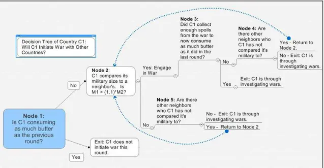
makeWar
After each unit has produced what it can, traded for as much additional wealth as it can, and spent a percentage of its total wealth in preparing its defenses then it does a self-check. This check is to see whether or not it has consumed what it has on average for the last five time periods plus 3% of that average.9If it has met this condition then the unit
(again, for clarity Unit1) will not instigate any wars. If Unit1 consumed less than that
amount, it will then run through a number of decisions about whether or not to go to war to see if it can to win, through war, the ability to consume what it could not through trade.
In deciding whether or not to go to war, Unit1 solicits the size of each visible unit’s army. It then selects the weakest unit (again Unit2 for purposes of clarity) and checks two conditions. First, Unit1 checks to see if its army is 10% stronger than the army of Unit2. Second, it checks to see if the spoils to be collected from Unit2 (20% of Unit2’s butter) are more than the cost of going to war (10% of Unit1’s army). If both these conditions hold, then Unit1 will instigate war. If either condition is false, then Unit1 will look to the next visible unit and ask the same questions.
20
Figure Two: The Decision Whether or Not to Initiate War
If Unit1 decides to go to war against Unit2, then the following series of calculations take place. First, an “advantage” variable is calculated by dividing the size of Unit1’s army by the sum of Unit1’s army and Unit2’s army.
advantage = (Unit 1’s ArmySize)/ (Unit 1’s ArmySize+ Unit 2’s ArmySize)
Because Unit1 only attacks countries with smaller armies “advantage” will always be greater than .5. Then a random number between zero and one is generated with a uniform
distribution. The attacking unit wins if the random number generated is less than the “advantage” variable. For example, if the attacker’s army is twice the size of the attacked, then the attacker has a two in three chance of wining.
eluded to earlier, both sides suffer a reduction in the size of their armies. The losing unit’s army is reduced by 20% and the winning unit’s army is reduced by 10%.
The unit whose turn it is then determines if it is now satisfied. If it is not, then it looks at the next visible unit and asks the same set of questions about whether or not to make war. When the unit is either satisfied or has exhausted its list of partners, it ceases to make war this round. In turn, the next unit decides whether or not to make war. When each unit has had its turn the next method is called.
resetRound
22
Table Three: Structure of a Round for Country C1
Action (or
method) Description Variables Created
In round one the amount of good A and the amount of good B are randomly set between 1 and 50. In all later rounds C1 produces 3% more of both goods (A and B) than it did in the previous round. C1 then determines how much it would like to trade with its partners by pairing one unit of A with one unit of B and placing any excess in a variable called AmountTradableC1 for later use.
AmountTradableC1
assess
C1 then creates a list of the countries it can interact with. The countries contained in this list are a function of the level of technology development of the system which is
exogenously given and increases every 50 rounds.
InteractionListC1(technology);
offerTrade
While C1 has goods to offer it sequentially asks each partner in InteractionListC1 if it would like to trade. If CXwould like to trade, C1 then reduces the amount it has to trade by the amount traded. When it has nothing less to trade then it stops looking for partners.
acceptTrade
C1 examines offers from other countries. If the offer is beneficial then C1 reduces AmountTradableC1 until
AmountTradableC1 = 0. When this occurs C1 no longer trades.
setDefense
C1 examines every county in
InteractionListC1. When another country has a larger army than C1, C1 builds its army to match the size of the opposing army. C1 will spend up to 1/2 of its GDP to create its army. At a minimum, C1 will spend 20% of its GDP on its army.
assessAgain
C1 subtracts how much it spent on its army to determine how much it can consume domestically. If that consumption is 3% less than the average of the previous five rounds, C1 is "dissatisfied."
Dissatisfied
makeWar
If C1 is dissatisfied, C1 looks through InteractionListC1 for weaker units. If C1 is 10% stronger than the other units (CX), C1
will start a war. The winner of the war is a randomly determined with C1's chance of winning increasing the larger its military is compared to CX's military. The winner
collects spoils from the loser and adds them to its consumption total. Both units lose a percentage of their armies during the
conflict. The winner loses 10% and the loser 20%.
resetRound
Dissatisfied, InteractionListC1, and
Chapter 3: General Patterns of Warfare
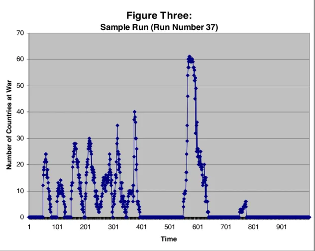
This section presents the output of the system as a whole to provide a general picture of how the system behaves. Given the assumptions and structure of the model, we expect war to initially be triggered by increases in trading technology. Some countries will find more preferable trading arrangements with new partners and therefore leave former partners. Figure One presents an example of the data output from a sample run of the model.
In this run, the predicted systemic pattern of warfare is occurring as expected. Wars occur after increases in transportation technology. As time passes the system returns to equilibrium. Increases in transportation technology early in the development of the system result in surges of war beginning at t = 51, 101, 151 . . . 350. From t = 400 to t= 550
subsequent improvements in transportation technology result in no wars. At t= 551 a major war begins. After t = 800 the system settles into a permanent peaceful equilibrium despite technological increases at t = 851, 900 and 951. This run suggests that changes in
Figure Three:
Sample Run (Run Number 37)
0 10 20 30 40 50 60 70
1 101 201 301 401 501 601 701 801 901
Time N u m b e r o f C o u n tr ie s a t W a r
26
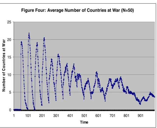
Figure Four: Average Number of Countries at War (N=50)
0 5 10 15 20 25
1 101 201 301 401 501 601 701 801 901
Time N u m b e r o f C o u n tr ie s a t W a r
Again, wars occur after increases in transportation technology. Table 2 suggests that the effects of increasing transportation technology differ over time. The average number of countries at war in time period 951 is considerably lower than those peaks occurring before t = 500.
Interestingly, when we further parse the results, we see that later in the system’s development the average number of wars is driven by large infrequent wars. Increases in transportation technology early in the run, almost always result in war. Increases in transportation technology later in the run, rarely result in war, but when these wars occur, they involve a large number of countries.
system’s development. Periods later in the system’s development are much less likely to have conflict.
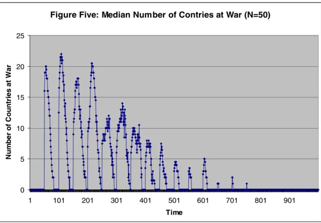
Figure Five: Median Number of Contries at War (N=50)
0 5 10 15 20 25
1 101 201 301 401 501 601 701 801 901
Time
N
u
m
b
e
r
o
f
C
o
u
n
tr
ie
s
a
t
W
a
r
28
Figure Six:
Minimum and Maximum Number of Countries at War (N=50)
0 10 20 30 40 50 60 70 80
1 101 201 301 401 501 601 701 801 901
Time N u m b e r o f C o u n tr ie s a t W a r
Minimum Across Sample Maximum Across Sample
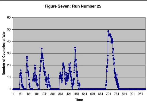
Figure Seven: Run Number 25
0 10 20 30 40 50 60
1 61 121 181 241 301 361 421 481 541 601 661 721 781 841 901 961
Time
N
u
m
b
e
r
o
f
C
o
u
n
tr
ie
s
a
t
W
a
Chapter 4: Causation of War in the System
The observations above show the general patterns of total countries at war in the system. I wish to investigate what predicts whether or not a country will start a war in any given period. Countries initiate war when consumption falls relative to historical levels. But as we have seen, the pattern of warfare seems to vary across time. The first step in an investigation is to see if this pattern can be statistically established. Is transportation technology negatively related to instigating war?
If transportation technology does have an effect on instigating wars, then the second question to answer is why does this relationship hold? Countries always go to war because they are deprived of butter consumption. What conditions make this deprivation more likely? What other variables could account for whether or not they make war? The empirical investigation below attempts to sort out these issues.
In order to test if there is a relationship between transportation technology and instigating war, I recorded the dependent variable, making war, and four independent variables: technology and three control variables. Each of these variables are recorded for each country in each time period.
If the relationship of transportation technology to conflict is established, I propose two mechanisms to explain why the frequency of wars falls over time as transportation technology increases:
Causal Mechanism 2: The farther each unit can see, the more likely it is that each unit can replace one lost trade partner with a new trade partner.
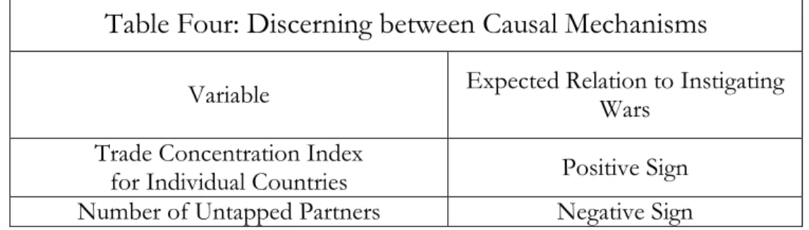
I created two variables to test these two causal mechanisms. First, if a concentration of trade variable was statistically linked to a decrease in the likelihood of a country to instigate wars, then there would be support for Causal Mechanism 1. Second, if a variable which captured the number of untapped trading partners was linked to a decrease in the likelihood of a country to instigate wars, then there would be support for Causal Mechanism 2. That is, if being connected to a greater number of countries enables a country to find new trading partners instead of incurring a loss, then the total number of untapped partners should be correlated with decreases in war instigation.
Table Four: Discerning between Causal Mechanisms
Variable Expected Relation to Instigating Wars Trade Concentration Index
for Individual Countries Positive Sign Number of Untapped Partners Negative Sign
The variables of interest are enumerated below. The reasoning behind their inclusion in the statistical analysis is provided in their description. The direction of their influence on the dependent variable is also hypothesized.
Dependent Variable
32
Independent Variables10
Technology measures how far each unit sees; it ranges between .05 and 1. Technology increases
by .05 every 50 time periods over the course of 1,000 time periods. The expected effect is unclear. It is possible that interacting with an increasing number of units will buffer trade shocks causing countries to make war less often. It is also possible that interacting with increasing numbers of units exposes countries to a greater number of warring countries. By losing resources in a war, countries might then be forced to go to war the next time period. The last possibility is that, by seeing more countries, the number of weak countries which a country would want to make war against increases.
Concentration of Trade is calculated in the following manner. First, the percentage of each
unit’s wealth due to trade is calculated by subtracting the pre-trading period wealth by the post-trade wealth and dividing by the post-trade wealth. If a country gets most of its wealth from trade, this number will trend towards a value of one. If little of a country’s wealth comes from trade, then this variable will trend towards zero. This percentage is then divided by the number of its trading partners. The measure reflects each unit’s average dependence on its partners where higher values indicate a higher level of dependence on a smaller number of countries. We expect this variable to take a positive sign.
10 Another variable was included in an initial analysis: Largest Army Two Links Away. It is possible that countries
Potential Trade Partners is the difference between the number of countries with which each
unit did trade and the total number of available trading partners. This difference is the number of countries which each unit could turn to in response to the loss of trade from one existing trade partners. We expect this variable to have a negative coefficient.
Armies Lost is the natural logarithm of number of armies each unit lost in war in the previous
round. Units replace armies lost in round T-1 with spending in round T. Because army size is in part a function of the economic size of a country and the economy grows exponentially, it was necessary to log the value. We expect this variable to take a negative sign.
Pre-War Army Size is the natural logarithm of the size of each unit’s military force after the
method setDefense is called and before makeWar is called. The larger a country’s army is, the more likely it is that it has a large military to be able to successfully initiate wars. As army size is in part a function of the economic size of a country and the economy grows
exponentially, it was necessary to log the raw value of this variable. We predict this variable to take a positive sign in predicting war.
Victim of War measures the number of times each unit has been attacked by other units in
34
Descriptive Statistics of the Variables
Table Five presents the descriptive statistics of the variables listed above. Armies Lost and Pre-War Army Size are presented after their transformation via the natural logarithm function.
Table Five: Descriptive Statistics of Variables Across All Observations
(9,990,000 observations per variable) Minimum Maximum Mean
Std. Error
Technology .05 1 0.525 0.288
Armies Lost (LN) -3.724 29.059 0.101 1.048
Victim of War 0 27 .058 .488
Pre-War Army Size (LN) -3.411 31.782 13.584 9.424
Concentration of Trade 0 .96 .242 0.224
Unused Partners 0 199 102.540 57.493 Results rounded to three decimal places.
Statistical Methods
Results
The first test I ran was to confirm that that increasing levels of transportation technology actually did have a significant and negative effect on the dependent variable madeWar. In order to do this I employed the following model:
madewar = madeWarUpon + preWarArmySize + Armies Lost + technology
The results of this model are displayed in Table Six. Unsurprisingly, the independent variables Armies Lost, Victim of War, and Pre-War Army Size were all significant at the .01 level in all 50 runs. Surprisingly, the sign for Pre-War Army-Size was negative, that is, having a larger army makes you less likely to instigate a war.
The other surprising result is that the effect of technology varied from run to run, with one run actually having technology be a strong predictor in the wrong direction. This occurred in run 9. An analysis of this run reveals an unusually low number of wars early in the simulation, high levels of warfare in the middle third, and a large war from t = 950 to t = 1,000.
Table Six: Number of Times Significant Out of
50 Runs Sign SignificantNot
Significant at the .1
level
Significant at the .05
level
Significant at the .01
level Outlier*
Armies Lost + - - - 50 -
Victim of War + - - - 50 -
Pre-War Army Size - - - - 50 -
Technology - 5 - 3 41 1*
Model Run: madewar= madeWarUpon + preWarArmySize + Armies Lost + technology; * In run 9 technology is significant at the .01 level but with a positive sign. An analysis of this run reveals an unusually low number of wars early in the simulation, high levels of warfare in the middle third, and a large war from t = 950 to t = 1,000
36
The descriptive statistics for the parameter estimates are displayed in Table Seven. The standard errors displayed in Table Seven are generated using the MIANALYZE procedure in SAS. Originally developed by Rubin (Rubin, 1987) to impute missing data by combining data sets the MIANALYZE procedure produces standard errors by combining the standard errors of both the individual parameters and the differences between the parameter estimates themselves.11
Table Seven: Descriptive Parameter Estimates of Variables Across All
Observations
(50 observations per parameter)
Minimum Maximum Mean Std. Error
Technology -1.597 0.396* -0.502 0.426
Armies Lost (LN) 0.654 1.120 0.902 0.113
Victim of War 0.484 1.696 1.323 0.179
Pre-War Army Size (LN) -0.613 -0.355 -0.455 0.057 Results rounded to three decimal places.
*This positive result occurs only once in the analysis of run 9. All other estimates of this parameter were negative.
The question of why increasing levels of technology result in less war was
investigated by removing technology from the logistic regression and inserting Concentration of Trade and Unused Partners to test the two causal mechanisms. The following model was used
and the results are displayed in Table Eight.
madeWar = madeWarUpon + preWarArmySize + Armies Lost + Concentration of Trade + Unused Partners
In this regression the three control variables, Armies Lost, Victim of War, and Pre-War Army Size, all maintained their signs and were significant at the .01 level in all 50 runs. The results
of the two independent variables were less uniform and are displayed in Table Eight. Unused Partners was significant in the correct direction in 92 percent of the runs and was
highly significant in 84 percent of the runs. Concentration of Trade preformed slightly less well. It was significant in the correct direction for 88 percent of the runs and highly significant in 78 percent of the runs.
Table Eight: Number of Times Significant Out of
50 Runs Sign
Not Significant
Significant at the.1 level
Significant at the .05
level
Significant at the .01
level Outlier Concentration of
Trade - 5 1 4 39 1*
Unused Partners - 2 0 4 42 2**
Armies Lost + - - - 50 -
Victim of War + - - - 50 -
Pre-War Army Size - - - - 50 -
Model Run:
madeWar = madeWarUpon + preWarArmySize + Armies Lost + Concentration of Trade + Unused Partners * For run 3 Concentration of Trade was positive and significant at the .1 level.
** For two runs Unused Partners took a positive value. Run 9 was significant at the .05 level and run 18 at .01 level.
38
Table Nine: Descriptive Parameter Estimates of Variables Across All
Observations
(50 observations per parameter)
Minimum Maximum Mean Std. Error
Concentration of Trade -0.112* 1.433 0.498 0.353 Unused Partners -0.009 0.001** -0.003 0.002
Armies Lost (LN) 0.644 1.102 0.892 0.114
Victim of War 0.487 1.691 1.318 0.178
Pre-War Army Size (LN) -0.591 -0.332 -0.443 0.056 Results rounded to three decimal places.
* The Concentration of Trade parameter took a negative sign for three runs: two insignificant and one significant at the .1 level. (Runs 23, 29 and 3 respectively).
Chapter 5: Conclusion
The results of the previous section suggest that the level of transportation
technology in a system can play an important effect on whether or not a country chooses to instigate war. In some runs the effect of technology (or its component parts) is highly significant. In other runs it has little effect. In one run, Run 9, higher levels of
transportation technology was a significant predictor of warfare. The variations in these findings are consistent with the variable findings in the literature. This model presents evidence that both the post-19th century analyses (finding trade is associated with peace) and
those that incorporate a larger time frame (finding that trade produces conflict) are correct, though the finding suggest a degree of spurious causation in the former.
This model provides support for several different streams of the political science literature. The significance of the Concentration of Trade variable provides support for the conclusion that countries that are highly dependent on a few countries for their welfare are more likely to be engaged in wars. (Barbieri, 1996)
40
Appendix -Illustrative Example of Three Countries over Three Rounds
This appendix provides an example of the mechanisms involved in the model using an example of two countries who engage in trade in rounds T and T+1. In round T+2 a third country is introduced and the effect explained.
Round T
In Round T, Saudi Arabia and the US have the productive capacity to produce two things, food and oil (food, oil). SA has (1,11) the US (11,1) We assume these goods are compliments and that these two countries want to trade. They swap 5 oils for 5 foods then have the following SA (6,6) and the US (6,6).
A country can spend its consumption on butter or guns. It sets its guns consumption based on what its neighbor does. As this is the first round, they would both build their armies to be .2 the size of their own economy. In this example the army size is .2*6 = 1.2. The amount left over is the butter it consumes as:
GDP – Guns = Butter
From Formula 1 we know that the butter is 4.8.
Round T SA US
Productive Capacity 1,11 11,1 Amount Produced 1,11 11,1
Amount Traded 5 5
Total Amount to be
Consumed 6 6
On Military 1.2 1.2
Round T+1
In Round T+1 each country’s productive capacity grows by .03. So far so good. Now the question is what to do with the army size (.2*6.18 = 1.236). Applying Formula 1 again we see that the butter for each country is now 4.944.
Round T+1 SA US
Productive Capacity 1.03,11.33 1.33,1.03 Amount Produced 1.03,11.33 11.33,1.03
Amount Traded 5.15 5.15
Total Amount to be
Consumed 6.18 6.18
On Military 1.236 1.236
On Butter 4.944 4.944
Round T+2:
In order to provide a picture of the dynamics produced by introducing new trading partners, this round complicates the story by introducing a third country to the trade group: Germany. Germany is randomly assigned the ability to produce five units of food and one unit of oil.
At the beginning of Round T+2 every one grows again. Then, when SA looks to trade if first trades with Germany 2 oils for 2 foods. Now SA only has 3.3 oils to trade with the US, dramatically driving down the US’s overall consumption.
42
chances of winning a war with both SA and Germany in the hopes of finding a weaker neighbor to capture resources from. Since the US is not 10% stronger than either neighbor it does not attempt to win a war and the round ends.
Round T+2 SA Germany US
Productive Capacity 1.061,11.67 5, 1 11.67, 1.061 Amount Produced 1.061,11.67 5, 1 11.67, 1.061
Amount Traded 2 + 3.3 = 5.3 2 3.3
Total Amount to be
Consumed 6.36 3 3.36
On Military 1.27 1.27 1.27
References
Barbieri, K. (1996). Economic Interdependence: A Path to Peace or a Source of Interstate Conflict? Journal of Peace Research, 33(1), 29.
Bearce, D. H., & Fisher, E. O. N. (2002). Economic Geography, Trade, and War. Journal of Conflict Resolution, 46(3), 365-393.
Beck, N., Katz, J. N., & Tucker, R. (1998). Taking Time Seriously: Time-series-cross-section analysis with a Binary Dependent Variable. American Journal of Political Science, 42(4), 1260-1288.
Bhavnani, R. (2003). Adaptive agents, Political Institutions and Civic Traditions in Modern Italy. [Electronic version]. Journal of Artificial Societies and Social Simulation, 6
Bremer, S. A., & Mihalka, M. (1977). Machiavelli in Machina: Or Politics among Hexagons. In K. W. Deutsch (Ed.), Problems of World Modeling. Boston: Ballinger.
Bueno de Mesquita, B. (2003). The Logic of Political Survival. Cambridge, Mass.: MIT Press. Cederman, L. E. (2005). Computational Models of Social Forms: Advancing Generative
Process Theory. American Journal of Sociology, 110(4), 864-893.
Cederman, L. (2001). Modeling the Democratic Peace as a Kantian Selection Process. Journal of Conflict Resolution, 45(4), 470-502.
Cederman, L. (2002). Back to Kant: Reinterpreting the Democratic Peace as a Macrohistorical Learning Process. American Political Science Review, 95(01), 15-31. Cederman, L. (2003). Modeling the Size of Wars: From Billiard Balls to Sandpiles. American
Political Science Review, 97(01), 135-150.
Cederman, L. (1997). Emergent Actors in World Politics: How States and Nations Develop and Dissolve. Princeton, N.J.: Princeton University Press.
Choucri, N., & North, R. C. (1975). Nations in Conflict: National Growth and International Violence. San Francisco: W. H. Freeman.
De Marchi, S. (2005). Computational and Mathematical Modeling in the Social Sciences. Cambridge, NY: Cambridge University Press.
Domke, W. K. (1988). War and the Changing Global System. New Haven: Yale University Press. Epstein, J. M. (1999). Agent-based Computational Models and Generative Social Science.
Complexity, 4(5), 41-60.
44
Fearon, J. D. (1995). Rationalist Explanations for War. International Organization, 49(3), 379-414.
Frieden, J. A. (2006). Global Capitalism: Its Fall and Rise in the Twentieth Century (1st ed.). New York: W.W. Norton.
Gasiorowski, M., & Polachek, S. W. (1982). Conflict and Interdependence: East-West Trade and Linkages in the Era of Detente. Journal of Conflict Resolution, 26(4), 709.
Gilpin, R. (1981). War and Change in World Politics. Cambridge; New York: Cambridge University Press.
Hart, D. B., & Munger, M. C. (1989). Declining Electoral Competitiveness in the House of Representatives: The Differential Impact of Improved Transportation Technology. Public Choice, 61(3), 217-228.
Hirschman, A. O. (1945). National Power and the Structure of Foreign Trade. Berkeley and Los Angeles: University of California Press.
Holsti, K. J. (1991). Peace and War: Armed Conflicts and International Order, 1648-1989. Cambridge; New York: Cambridge University Press.
Hugill, P. J. (1993). World Trade Since 1431: Geography, Technology, and Capitalism. Baltimore: Johns Hopkins University Press.
Jervis, R. (1997). System Effects: Complexity in Political and Social Life. Princeton, N.J.: Princeton University Press.
Kant, I., & Smith, M. C. (1903). Perpetual Peace: a Philosophical Essay (1.th ed.). London: G. Allen & Unwin.
Keohane, R. O., & Nye, J. S. (2001). Power and Interdependence (3rd ed.). New York: Longman. Kollman, K., Miller, J. H., & Page, S. E. (2003). Computational Models in Political Economy.
Cambridge, Mass.: MIT Press.
Krugman, P. R., & Obstfeld, M. (2003). International Economics:Theory and Policy (6th ed.). Boston: Addison Wesley.
Levy, J. S. (1999). "The Rise and Decline of the Anglo-Dutch Rivalry, 1609-1689. In W. R. Thompson (Ed.), Great Power Rivalries (pp. 172-200). Columbia: University of South Carolina Press.
Levy, J. S., & Ali, S. (1998). From Commercial Competition to Strategic Rivalry to War: The Evolution of the Anglo-Dutch Rivalry, 1609–1652. In P. F. Diehl (Ed.), The Dynamics of Enduring Rivalries (pp. 29–63). Urbana: University of Illinois Press.
Lustick, I. S., Miodownik, D., & Eidelson, R. J. (2004). Secessionism in Multicultural States: Does Sharing Power Prevent or Encourage It? American Political Science Review, 98(02), 209-229.
Mansfield, E. D. (1994). Power, Trade, and War. Princeton, N.J.: Princeton University Press. Mansfield, E. D., & Pollins, B. (2003). Economic Interdependence and International Conflict: New
Perspectives on an Enduring Debate. Ann Arbor: University of Michigan Press.
McMillian, S. (1997). "Interdependence and Conflict". Mershon International Studies Review, 41, 33-58.
Milner, H. V. (1999). “The Political Economy of International Trade.” Annual Review of Political Science, 2(1), 91-114.
Morrow, J. D. (1989). Capabilities, Uncertainty, and Resolve: A Limited Information Model of Crisis Bargaining. American Journal of Political Science, 33(4), 941-972.
Oatley, T. H. (2006). International Political Economy: Interests and Institutions in the Global Economy (2nd ed.). New York: Pearson/Longman.
Oneal, J. R., Oneal, F. H., Maoz, Z., & Russett, B. (1996). The Liberal Peace:
Interdependence, Democracy, and International Conflict, 1950-85. Journal of Peace Research, 33(1), 11.
Oneal, J. R., & Russett, B. M. (1997). The Classical Liberals were Right: Democracy,
Interdependence, and Conflict, 1950-1985. International Studies Quarterly, 41(2), 267-293. Oneal, J. R., & Russett, B. M. (1999a). Assessing the Liberal Peace with Alternative
Specifications: Trade Still Reduces Conflict. Journal of Peace Research, 36(4), 423-442. Oneal, J. R., & Russett, B. M. (1999b). The Kantian Peace: The Pacific Benefits of
Democracy, Interdependence, and International Organizations, 1885-1992. World Politics, 52(1), 1-37.
Penubarti, M., & Ward, M. D. (2000). Commerce and Democracy. Unpublished manuscript. Polacheck, S. (1980). Conflict and Trade. Journal of Conflict Resolution, 24, 55-78.
Polachek, S. W., Robst, J., & Chang, Y. C. (1999). Liberalism and Interdependence: Extending the Trade-Conflict Model. Journal of Peace Research, 36(4), 405-422.
Pollins, B. M., & Kirkpatrick, G. (1987). Modeling an international trade system. In C. A. Cioffi-Revilla, R. L. Merritt & D. A. Zinnes (Eds.), Communication and Interaction in Global Politics (pp. 65–88). Beverly Hills: Sage Publications.
46
Rubin, D. B. (1987). Multiple Imputation for Nonresponse in Surveys. New York: Wiley. Schafer, J. L. (1997). Analysis of Incomplete Multivariate Data (1st ed.). London; New York:
Chapman & Hall.
Stein, A. A. (1993). Governments, Economic Interdependence, and International
Cooperation. In Philip E. Tetlock, Jo L. Husbands, Robert Jervis, Paul C. Stern, and Charles Tilly (Ed.), Behavior, Society, and Nuclear War (pp. 241–324). New York: Oxford University Press.
Stoll, R. J. (1987). System and State in International Politics: A Computer Simulation of Balancing in an Anarchic World. International Studies Quarterly, 31(4), 387-402. Taber, C. S., & Timpone, R. J. (1996). Beyond Simplicity: Focused Realism and
Computational Modeling in International Relations. Mershon International Studies Review, 40(1), 41-79.
Viner, J. (1948). Power versus Plenty as Objectives of Foreign Policy in the Seventeenth and Eighteenth Centuries. World Politics, 1(1), 1-29.