Mismatched Decoding: Error Exponents,
Second-Order Rates and Saddlepoint Approximations
Jonathan Scarlett, Alfonso Martinez,
Senior Member, IEEE, and Albert Guillén i Fàbregas,
Senior Member, IEEE
Abstract—This paper considers the problem of channel coding with a given (possibly suboptimal) maximum-metric decoding rule. A cost-constrained random-coding ensemble with multiple auxiliary costs is introduced, and is shown to achieve error expo-nents and second-order coding rates matching those of constant-composition random coding, while being directly applicable to channels with infinite or continuous alphabets. The number of auxiliary costs required to match the error exponents and second-order rates of constant-composition coding is studied, and is shown to be at most two. For i.i.d. random coding, asymptotic estimates of two well-known non-asymptotic bounds are given using saddlepoint approximations. Each expression is shown to characterize the asymptotic behavior of the corresponding random-coding bound at both fixed and varying rates, thus unifying the regimes characterized by error exponents, second-order rates and moderate deviations. For fixed rates, novel exact asymptotics expressions are obtained to within a multiplicative
1 +o(1) term. Using numerical examples, it is shown that the saddlepoint approximations are highly accurate even at short block lengths.
Index Terms—Mismatched decoding, random coding, error exponents, second-order coding rate, channel dispersion, normal approximation, saddlepoint approximation, exact asymptotics, maximum-likelihood decoding, finite-length performance
I. INTRODUCTION
Information-theoretic studies of channel coding typically seek to characterize the performance of coded communication systems when the encoder and decoder can be optimized. In practice, however, optimal decoding rules are often ruled out due to channel uncertainty and implementation constraints. In this paper, we consider the mismatched decoding problem [1]– [8], in which the decoder employs maximum-metric decoding with a metric which may differ from the optimal choice.
The problem of finding the highest achievable rate possible with mismatched decoding is open, and is generally believed to be difficult. Most existing work has focused on achievable
J. Scarlett is with the Department of Engineering, University of Cam-bridge, CamCam-bridge, CB2 1PZ, U.K. (e-mail: [email protected]). A. Martinez is with the Department of Information and Communication Tech-nologies, Universitat Pompeu Fabra, 08018 Barcelona, Spain (e-mail: [email protected]). A. Guillén i Fàbregas is with the Institució Cata-lana de Recerca i Estudis Avançats (ICREA), the Department of Informa-tion and CommunicaInforma-tion Technologies, Universitat Pompeu Fabra, 08018 Barcelona, Spain, and also with the Department of Engineering, University of Cambridge, Cambridge, CB2 1PZ, U.K. (e-mail: [email protected]). This work has been funded in part by the European Research Council under ERC grant agreement 259663, by the European Union’s 7th Framework Programme under grant agreement 303633 and by the Spanish Ministry of Economy and Competitiveness under grants RYC-2011-08150 and TEC2012-38800-C03-03. This work was presented in part at the Allerton Conference on Communication, Computing and Control (2012), and at the Information Theory and Applications Workshop (2013, 2014).
rates via random coding; see Section I-C for an outline. The goal of this paper is to present a more comprehensive analysis of the random-coding error probability under various ensembles, including error exponents [9, Ch. 5], second-order coding rates [10]–[12], and refined asymptotic results based on the saddlepoint approximation [13].
A. System Setup
The input and output alphabets are denoted by X and
Y respectively. The conditional probability of receiving an output vector y = (y1,· · ·, yn) given an input vector x = (x1,· · ·, xn)is given by
Wn(y|x), n Y
i=1
W(yi|xi) (1)
for some transition law W(y|x). Except where stated oth-erwise, we assume that X and Y are finite, and thus the channel is a discrete memoryless channel (DMC). The encoder takes as input a message m uniformly distributed on the set
{1, . . . , M}, and transmits the corresponding codewordx(m)
from a codebookC={x(1), . . . ,x(M)}. The decoder receives the vector y at the output of the channel, and forms the estimate
ˆ
m= arg max j∈{1,...,M}
qn(x(j),y), (2) where qn(x,y)
, Qn
i=1q(xi, yi). The function q(x, y) is assumed to be non-negative, and is called thedecoding metric. In the case of a tie, a codeword achieving the maximum in (2) is selected uniformly at random. It should be noted that maximum-likelihood (ML) decoding is a special case of (2), since it is recovered by setting q(x, y) =W(y|x).
An error is said to have occurred ifmˆ differs from m. A rate R is said to be achievable if, for all δ >0, there exists a sequence of codes Cn of length n withM ≥en(R−δ) and vanishing error probabilitype(Cn). An error exponentE(R)is said to be achievable if there exists a sequence of codebooks
Cn of lengthn and rateR such that
lim inf n→∞ −
1
nlogpe(Cn)≥E(R). (3)
We let pe(n, M) denote the average error probability with respect to a given random-coding ensemble which will be clear from the context. The random-coding error exponent Er(R) is said to exhibit ensemble tightness if
lim n→∞−
1
nlogpe(n, e
nR) =E
B. Notation
The set of all probability distributions on an alphabet X is denoted by P(X), and the set of all empirical distributions on a vector inXn (i.e. types [14, Sec. 2] [15]) is denoted by Pn(X). The type of a vector x is denoted by Pˆx(·). For a
givenQ∈ Pn(X), the type classTn(Q)is defined to be the set of all sequences in Xn with typeQ.
The probability of an event is denoted by P[·], and the
symbol ∼ means “distributed as”. The marginals of a joint distributionPXY(x, y)are denoted byPX(x)andPY(y). We writePX =PeX to denote element-wise equality between two probability distributions on the same alphabet. Expectation with respect to a joint distribution PXY(x, y) is denoted by EP[·], or E[·] when the associated probability distribution
is understood from the context. Similar notations IP(X;Y) and I(X;Y) are used for the mutual information. Given a distribution Q(x) and conditional distribution W(y|x), we writeQ×W to denote the joint distributionQ(x)W(y|x).
For two positive sequences fn and gn, we write fn
.
=
gn if limn→∞n1loggfnn = 0, and we write fn≤˙ gn if lim supn→∞n1logfn
gn ≤ 0 and analogously for
˙
≥. We write
fngn iflimn→∞fgnn = 1, and we make use of the standard asymptotic notationsO(·),o(·),Θ(·),Ω(·)andω(·).
We denote the tail probability of a zero-mean unit-variance Gaussian variable byQ(·), and we denote its functional inverse byQ−1(·). All logarithms have basee, and all rates are in units of nats except in the examples, where bits are used. We define
[c]+= max{0, c}, and denote the indicator function by11{·}.
C. Overview of Achievable Rates
Achievable rates for mismatched decoding have been de-rived using the following random-coding ensembles:
1) the i.i.d. ensemble, in which each symbol of each code-word is generated independently;
2) the constant-composition ensemble, in which each code-word is drawn uniformly from the set of sequences with a given empirical distribution;
3) the cost-constrained ensemble, in which each codeword is drawn according to an i.i.d. distribution conditioned on an auxiliary cost constraint being satisfied.
While these ensembles all yield the same achievable rate under ML decoding, i.e. the mutual information, this is not true under mismatched decoding.
The most notable early works on mismatched decoding are by Hui [2] and Csiszár and Körner [1], who used constant-composition random coding to derive the following achievable rate for mismatched DMCs, commonly known as the LM rate:
ILM(Q) = min
e
PXY
I e
P(X;Y), (5)
where the minimization is over all joint distributions satisfying
e
PX(x) =Q(x) (6)
e
PY(y) = X
x
Q(x)W(y|x) (7)
EPe[logq(x, y)]≥EQ×W[logq(x, y)]. (8)
This rate can equivalently be expressed as [7]
ILM(Q), sup s≥0,a(·)
E
log q(X, Y) sea(X)
E[q(X, Y)sea(X)|Y]
, (9)
where(X, Y, X)∼Q(x)W(y|x)Q(x).
Another well-known rate in the literature is the generalized mutual information (GMI) [3], [7], given by
IGMI(Q) = min
e
PXY
D PeXYkQ×PeY
, (10)
where the minimization is over all joint distributions satisfying (7) and (8). This rate can equivalently be expressed as
IGMI(Q),sup s≥0E
log q(X, Y) s E[q(X, Y)s|Y]
. (11)
Both (10) and (11) can be derived using i.i.d. random coding, but only the latter has been shown to remain valid in the case of continuous alphabets [3].
The GMI cannot exceed the LM rate, and the latter can be strictly higher even after the optimization of Q. Motivated by this fact, Ganti et al. [7] proved that (9) is achievable in the case of general alphabets. This was done by gen-erating a number of codewords according to an i.i.d. dis-tribution Q, and then discarding all of the codewords for which 1nP
n
i=1a(xi)−EQ[a(X)]
exceeds some threshold.
An alternative proof is given in [16] using cost-constrained random coding.
In the terminology of [7], (5) and (10) are primal expres-sions, and (9) and (11) are the corresponding dual expressions. Indeed, the latter can be derived from the former using Lagrange duality techniques [5], [17].
For binary-input DMCs, a matching converse to the LM rate was reported by Balakirsky [6]. However, in the general case, several examples have been given in which the rate is strictly smaller than the mismatched capacity [4], [5], [8]. In particular, Lapidoth [8] gave an improved rate using multiple-access coding techniques. See [18], [19] for more recent studies on the benefit of multiuser coding techniques, [20] for a study of expurgated exponents, and [21] for multi-letter converse results.
D. Contributions
Motivated by the fact that most existing work on mis-matched decoding has focused on achievable rates, the main goal of this paper is to present a more detailed analysis of the random-coding error probability. Our main contributions are as follows:
1) In Section II, we present a generalization of the cost-constrained ensemble in [9, Ch 7.3], [16] to include multiple auxiliary costs. This ensemble serves as an alternative to constant-composition codes for improving the performance compared to i.i.d. codes, while being ap-plicable to channels with infinite or continuous alphabets. 2) In Section III, an ensemble-tight error exponent is given for the cost-constrained ensemble. It is shown that the exponent for the constant-composition ensemble [1] can be recovered using at most two auxiliary costs, and sometimes fewer.
3) In Section IV, an achievable second-order coding rate is given for the cost-constrained ensemble. Once again, it is shown that the performance of constant-composition coding can be matched using at most two auxiliary costs, and sometimes fewer. Our techniques are shown to provide a simple method for obtaining second-order achievability results for continuous channels.
4) In Section V, we provide refined asymptotic results for i.i.d. random coding. For two non-asymptotic random-coding bounds introduced in Section II, we give sad-dlepoint approximations [13] that can be computed ef-ficiently, and that characterize the asymptotic behavior of the corresponding bounds as n → ∞ at all positive rates (possibly varying withn). In the case of fixed rates, the approximations recover the prefactor growth rates obtained by Altu˘g and Wagner [22], along with a novel characterization of the multiplicative O(1) terms. Using numerical examples, it is shown that the approximations are remarkably accurate even at small block lengths.
II. RANDOM-CODINGBOUNDS ANDENSEMBLES
Throughout the paper, we consider random coding in which each codeword X(i)(i= 1,· · ·, M) is independently gener-ated according to a given distribution PX. We will frequently
make use of the following theorem, which provides variations of the random-coding union (RCU) bound given by Polyanskiy et al. [11].
Theorem 1. For any codeword distributionPX(x)and
con-stant s≥0, the random-coding error probability pe satisfies
1
4rcu(n, M)≤pe(n, M)≤rcu(n, M)≤rcus(n, M), (12)
where
rcu(n, M),E min
1,
(M−1)P[qn(X,Y)≥qn(X,Y)|X,Y] (13)
rcus(n, M),E
minn1,(M −1)E[q
n(X,Y)s|Y]
qn(X,Y)s o
(14) with(X,Y,X)∼PX(x)Wn(y|x)PX(x).
Proof: Similarly to [11], we obtain the upper boundrcu
by writing
pe(n, M)≤P
[
i6=m
qn(X(i),Y)≥qn(X,Y)
(15)
=E "
P
[
i6=m
qn(X(i),Y)≥qn(X,Y) X,Y
#
(16)
≤rcu(n, M), (17) where (15) follows by upper bounding the random-coding error probability by that of the decoder which breaks ties as errors, and (17) follows by applying the truncated union bound. To prove the lower bound in (12), it suffices to show that each of the upper bounds in (15) and (17) is tight to within a factor of two. The matching lower bound to (15)
follows since whenever a tie occurs it must be between at least two codewords [23], and the matching lower bound to (17) follows since the union is over independent events [24, Lemma A.2]. We obtain the upper bound rcus by applying Markov’s inequality to the inner probability in (13).
In this paper, we consider the cost-constrained ensemble characterized by the following codeword distribution:
PX(x) =
1
µn n Y
i=1
Q(xi)11
x∈ Dn , (18)
where
Dn,
x : 1
n
n X
i=1
al(xi)−φl
≤ δ
n, l= 1, . . . , L
, (19) and where µn is a normalizing constant, δ is a positive constant, and for each l = 1, . . . , L, al(·) is a real-valued function on X, and φl , EQ[al(X)]. We refer to each functional(·)as an auxiliary cost function, or simply a cost. Roughly speaking, each codeword is generated according to an i.i.d. distribution conditioned on the empirical mean of each cost function al(x) being close to the true mean. This generalizes the ensemble studied in [9, Sec. 7.3], [16] by including multiple costs.
The cost functions{al(·)}Ll=1 in (18) should not be viewed as being chosen to meet a system constraint (e.g. power lim-itations). Rather, they are introduced in order to improve the performance of the random-coding ensemble itself. However, system costs can be handled similarly; see Section VI for details. The constantδin (18) could, in principle, vary withl
andn, but a fixed value will suffice for our purposes. In the case that L = 0, it should be understood that Dn contains all x sequences. In this case, (18) reduces to the i.i.d. ensemble, which is characterized by
PX(x) =
n Y
i=1
Q(xi). (20)
A less obvious special case of (18) is the constant-composition ensemble, which is characterized by
PX(x) =
1 |Tn(Q
n)|
11x∈Tn(Qn) , (21)
whereQn is a type such thatmaxx|Qn(x)−Q(x)| ≤ n1. That is, each codeword is generated uniformly over the type class
Tn(Q
n), and hence each codeword has the same composition. To recover this ensemble from (18), we replaceQbyQn and choose the parametersL=|X |,δ <1 and
al(x) =11{x=l}, l= 1,· · · ,|X |, (22) where we assume without loss of generality that X = {1,· · ·,|X |}.
The following proposition shows that the normalizing con-stantµn in (18) decays at most polynomially inn. When|X | is finite, this can easily be shown using the method of types. In particular, choosing the functions given in the previous paragraph to recover the constant-composition ensemble, we have µn ≥ (n + 1)−(|X |−1) [14, p. 17]. For the sake of generality, we present a proof which applies to more general
alphabets, subject to minor technical conditions. The case
L= 1was handled in [9, Ch. 7.3].
Proposition 1. Fix an input alphabet X (possibly infinite or continuous), an input distributionQ∈ P(X)and the auxiliary cost functions a1(·),· · · , aL(·). If EQ[al(X)2]< ∞ for l = 1, . . . , L, then there exists a choice of δ > 0 such that the normalizing constant in (18)satisfiesµn = Ω(n−L/2).
Proof:This result follows from the multivariate local limit theorem in [25, Cor. 1], which gives asymptotic expressions for probabilities of i.i.d. random vectors taking values in sets of the form (19). LetΣdenote the covariance matrix of the vector
[a1(X), . . . , aL(X)]T. We have by assumption that the entries of Σare finite. Under the additional assumptiondet(Σ)>0, [25, Cor. 1] states that µn = Θ(n−L/2) provided thatδ is at least as high as the largest span of theal(X)(X ∼Q) which are lattice variables.1If all such variables are non-lattice, then
δ can take any positive value.
It only remains to handle the casedet(Σ) = 0. Suppose that
Σhas rankL0 < L, and assume without loss of generality that
a1(·),· · · , aL0(·) are linearly independent. Up to sets whose probability with respect to Q is zero, the remaining costs
aL0+1(·),· · ·, aL(·)can be written as linear combinations of the firstL0costs. Lettingαdenote the largest magnitude of the scalar coefficients in these linear combinations, we conclude that x∈ Dn provided that
1
n
n X
i=1
al(xi)−φl
≤ δ
αL0n (23)
for l = 1,· · ·, L0. The proposition follows by choosing δ to be at least as high asαL0 times the largest span of theal(X) which are lattice variables, and analyzing the first L0 costs analogously to the case that det(Σ)>0.
In accordance with Proposition 1, we henceforth assume that the choice ofδ for the cost-constrained ensemble is such that µn= Ω(n−L/2).
III. RANDOM-CODINGERROREXPONENTS
Error exponents characterize the asymptotic exponential behavior of the error probability in coded communication sys-tems, and can thus provide additional insight beyond capacity results. In the matched setting, error exponents were studied by Fano [26, Ch. 9] and later by Gallager [9, Ch. 5] and Csiszár-Körner [14, Ch. 10]. The ensemble tightness of the exponent (cf. (4)) under ML decoding was studied by Gallager [27] and D’yachkov [28] for the i.i.d. and constant-composition ensembles respectively.
In this section, we present the ensemble-tight error exponent for cost-constrained random coding, yielding results for the i.i.d. and constant-composition ensembles as special cases.
1 We say thatX is a lattice random variable with offsetγand spanhif its support is a subset of{γ+ih:i∈Z}, and the same cannot remain true by increasingh.
A. Cost-Constrained Ensemble We define the sets
S({al}),
PXY ∈ P(X × Y) :
EP[al(X)] =φl, l= 1,· · ·, L (24) T(PXY,{al}),
n e
PXY ∈ P(X × Y) :
EPe[al(X)] =φl(l= 1,· · ·, L),PeY =PY,
EPe[logq(X, Y)]≥EP[logq(X, Y)]
o
, (25) where the notation {al} is used to denote dependence on
a1(·),· · ·, aL(·). The dependence of these sets on Q (via
φl=EQ[al(X)]) is kept implicit.
Theorem 2. The random-coding error probability for the cost-constrained ensemble in(18)satisfies
lim n→∞−
1
nlogpe(n, e
nR) =Ecost
r (Q, R,{al}), (26)
where
Ercost(Q, R,{al}), min PXY∈S({al})
min
e
PXY∈T(PXY,{al})
D(PXYkQ×W) +D(PeXYkQ×PY)−R +
. (27) Proof:See Appendix A.
The optimization problem in (27) is convex when the input distribution and auxiliary cost functions are fixed. The following theorem gives an alternative expression based on Lagrange duality [17].
Theorem 3. The error exponent in (27)can be expressed as
Ecostr (Q, R,{al}) = max ρ∈[0,1]
E0cost(Q, ρ,{al})−ρR, (28)
where
E0cost(Q, ρ,{al}), sup s≥0,{rl},{rl}
−logE "
Eq(X, Y)se
PL
l=1rl(al(X)−φl)|Y
q(X, Y)sePL
l=1rl(al(X)−φl)
ρ#
(29)
and (X, Y, X)∼Q(x)W(y|x)Q(x). Proof:See Appendix B.
The derivation of (28)–(29) via Theorem 2 is useful for proving ensemble tightness, but has the disadvantage of being applicable only in the case of finite alphabets. We proceed by giving a direct derivation which does not prove ensemble tightness, but which extends immediately to more general alphabets provided that the second moments associated with the cost functions are finite (see Proposition 1). The extension to channels with input constraints is straightforward; see Section VI for details.
Using Theorem 1 and applyingmin{1, α} ≤αρ(ρ∈[0,1]) torcus in (14), we obtain2
pe(n, M)≤ 1
µ1+n ρ
Mρ X
x∈Dn,y
Qn(x)Wn(y|x)
× P
x∈DnQ
n(x)qn(x,y)s
qn(x,y)s
ρ
, (30) whereQn(x),Qn
i=1Q(xi). From (19), each codewordx∈ Dn satisfies
er(anl(x)−nφl)e|r|δ≥1 (31) for any real numberr, wherean
l(x), Pn
i=1al(xi). Weaken-ing (30) by applyWeaken-ing (31) multiple times, we obtain
pe(n, M)≤
eρP
l(|rl|+|rl|)δ
µ1+n ρ
Mρ X
x∈Dn,y
Qn(x)Wn(y|x)
× P
x∈DnQ
n(x)qn(x,y)seP
lrl(anl(x)−nφl)
qn(x,y)seP
lrl(anl(x)−nφl)
!ρ
, (32)
where{rl}and{rl}are arbitrary. Further weakening (32) by replacing the summations over Dn with summations over all sequences, and expanding each term in the outer summation as product fromi= 1ton, we obtain
pe(n, M)≤e ρP
l(|rl|+|rl|)δ
µ1+n ρ
Mρ X
x,y
Q(x)W(y|x)
× P
xQ(x)q(x, y) seP
lrl(al(x)−φl)
q(x, y)seP
lrl(al(x)−φl)
!ρ!n
. (33) Sinceµndecays to zero subexponentially inn(cf. Proposition 1), we conclude that the prefactor in (33) does not affect the exponent. Hence, and setting M =enR, we obtain (28).
The preceding analysis can be considered a refinement of that of Shamai and Sason [16], who showed that an achievable error exponent in the case thatL= 1is given by
Ercost0(Q, R, a1), max ρ∈[0,1]E
cost0
0 (Q, ρ, a1)−ρR, (34) where
E0cost0(Q, ρ, a1),sup s≥0
−logE "
E[q(X, Y)sea1(X)|Y]
q(X, Y)sea1(X) !ρ#
.
(35) By settingr1=r1= 1in (29), we see thatErcostwithL= 1 is at least as high as Ecost0
r . In Section III-C, we show that the former can be strictly higher.
B. i.i.d. and Constant-Composition Ensembles
Setting L= 0 in (29), we recover the exponent of Kaplan and Shamai [3], namely
Eriid(Q, R), max ρ∈[0,1]E
iid
0 (Q, ρ)−ρR, (36)
2In the case of continuous alphabets, the summations should be replaced by integrals.
where
Eiid0 (Q, ρ),sup s≥0
−logE "
Eq(X, Y)s|Y
q(X, Y)s
ρ#
. (37) In the special case of constant-composition random coding (see (21)–(22)), the constraints EPe[al(X)] = φl for l =
1,· · ·,|X | yield PX = Q and PeX = Q in (24) and (25) respectively, and thus (27) recovers Csiszár’s exponent for constant-composition coding [1]. Hence, the exponents of [1], [3] are tight with respect to the ensemble average.
We henceforth denote the exponent for the constant-composition ensemble byEcc
r (Q, R). We claim that
Ercc(Q, R) = max ρ∈[0,1]E
cc
0 (Q, ρ)−ρR, (38) where
E0cc(Q, ρ) = sup s≥0,a(·)
E "
−logE
Eq(X, Y)sea(X)|Y
q(X, Y)sea(X)
ρ
X
#
. (39) To prove this, we first note from (22) that
X
l
rl(al(x)−φl) = X
e
x
r e
x(11{x=xe} −Q(xe)) (40) =r(x)−φr, (41) where (40) follows sinceφl=EQ[11{x=l}] =Q(l), and (41) follows by definingr(x),rx andφr,EQ[r(X)]. Defining
r(x) and φr similarly, we obtain the following E0 function from (29):
E0cc(Q, ρ), sup s≥0,r(·),r(·)
−logX x,y
Q(x)W(y|x)
× P
xQ(x)q(x, y)
ser(x)−φr
q(x, y)ser(x)−φr
ρ
(42)
≤ sup s≥0,r(·),r(·)
−X x
Q(x) logX y
W(y|x)
× P
xQ(x)q(x, y)
ser(x)−φr
q(x, y)ser(x)−φr
ρ
(43)
= sup s≥0,r(·)
−X x
Q(x) logX y
W(y|x)
× P
xQ(x)q(x, y) ser(x)
q(x, y)ser(x)
ρ
, (44)
where (43) follows from Jensen’s inequality, and (44) follows by using the definitions ofφr andφr to write
−X x
Q(x) log
e−φr
er(x)−φr
ρ
=−X x
Q(x) log 1
er(x)
ρ
.
(45) Renaming r(·) as a(·), we see that (44) coincides with (39). It remains to show that equality holds in (43). This is easily seen by noting that the choice
r(x) =1
ρlog
X
y
W(y|x) P
xQ(x)q(x, y) ser(x)
q(x, y)s
ρ
makes the logarithm in (43) independent of x, thus ensuring that Jensen’s inequality holds with equality.
The exponent Eiid
r (Q, R) is positive for all rates below
IGMI(Q)[3], whereasErccrecovers the stronger rateILM(Q). Similarly, bothEcost
r (L= 1) andEcost
0
r recover the LM rate provided that the auxiliary cost is optimized [16].
C. Number of Auxiliary Costs Required We claim that
Eriid(Q, R)≤E cost
r (Q, R,{al})≤Ercc(Q, R). (47) The first inequality follows by settingrl=rl= 0in (29), and the second inequality follows by setting r(x) = P
lrlal(x) and r(x) = P
lrlal(x) in (29), and upper bounding the objective by taking the supremum over all r(·) and r(·) to recover Ecc
0 in the form given in (42). Thus, the constant-composition ensemble yields the best error exponent of the three ensembles.
In this subsection, we study the number of auxiliary costs required for cost-constrained random coding to achieve Ercc. Such an investigation is of interest in gaining insight into the codebook structure, and since the subexponential prefactor in (33) grows at a slower rate whenLis reduced (see Proposition 1). Our results are summarized in the following theorem.
Theorem 4. Consider a DMCW and input distributionQ. 1) For any decoding metric, we have
sup a1(·),a2(·)
Ercost(Q, R,{a1, a2}) =Eccr (Q, R) (48)
max Q asup
1(·)
Ercost0(Q, R, a1) = max
Q E
cc
r (Q, R). (49) 2) If q(x, y) =W(y|x)(ML decoding), then
sup a1(·)
Ecostr (Q, R, a1) =Ercc(Q, R) (50) sup
a1(·)
Ercost0(Q, R, a1) =Eriid(Q, R) (51) max
Q E
iid
r (Q, R) = max
Q E
cc
r (Q, R). (52) Proof: We have from (47) that Ecost
r ≤Ercc. To obtain the reverse inequality corresponding to (48), we set L = 2,
r1=r2= 1andr2=r1= 0 in (29). The resulting objective coincides with (42) upon settinga1(·) =r(·)anda2(·) =r(·). To prove (49), we note the following observation from Appendix C: Given s > 0 and ρ > 0, any pair (Q, a)
maximizing the objective in (39) must satisfy the property that the logarithm in (39) has the same value for all xsuch that
Q(x)>0. It follows that the objective in (39) is unchanged when the expectation with respect to X is moved inside the logarithm, thus yielding the objective in (35).
We now turn to the proofs of (50)–(52). We claim that, under ML decoding, we can write Ecc
0 as
E0cc(Q, ρ) = sup a(·)
−logX y
X
x
Q(x)W(y|x)1+1ρea(x)−φa
1+ρ
, (53)
where φa , EQ[a(X)]. To show this, we make use of the form ofEcc
0 given in (42), and write the summation inside the logarithm as
X
y
X
x
Q(x)W(y|x)1−sρe−ρ(r(x)−φr)
×
X
x
Q(x)W(y|x)ser(x)−φr
ρ
. (54) Using Hölder’s inequality in an identical fashion to [9, Ex. 5.6], this summation is lower bounded by
X
y
X
x
Q(x)W(y|x)1+1ρer(x)−φr
1+ρ
(55)
with equality if and only if s = 1+1ρ and r(·) = −ρr(·). Renamingr(·)asa(·), we obtain (53). We can clearly achieve
Ecc
r using L = 2 with the cost functions r(·) and r(·). However, since we have shown that one is a scalar multiple of the other, we conclude that L= 1suffices.
A similar argument using Hölder’s inequality reveals that the objective in (35) is maximized bys=1+1ρ anda1(·) = 0, and the objective in (37) is maximized by s = 1+1ρ, thus yielding (51). Finally, combining (49) and (51), we obtain (52). Theorem 4 shows that the cost-constrained ensemble recov-ers Ecc
r using at most two auxiliary costs. If either the input distribution or decoding rule is optimized, thenL= 1suffices (see (49) and (50)), and if both are optimized then L = 0
suffices (see (52)). The latter result is well-known [15] and is stated for completeness. While (49) shows that Ercost and
Ercost0 coincide whenQis optimized, (50)–(51) show that the former can be strictly higher for a givenQeven whenL= 1, sinceErcccan exceed Eriid even under ML decoding [15].
D. Numerical Example
We consider the channel defined by the entries of the|X | × |Y|matrix
1−2δ0 δ0 δ0
δ1 1−2δ1 δ1
δ2 δ2 1−2δ2
(56)
with X = Y = {0,1,2}. The mismatched decoder chooses the codeword which is closest to y in terms of Hamming distance. For example, the decoding metric can be taken to be the entries of (56) with δi replaced by δ∈(0,13) for i= 1,2,3. We let δ0 = 0.01, δ1 = 0.05, δ2 = 0.25 and Q =
(0.1,0.3,0.6). Under these parameters, we have IGMI(Q) =
0.387,ILM(Q) = 0.449 andI(X;Y) = 0.471 bits/use. We evaluate the exponents using the optimization software YALMIP [29]. For the cost-constrained ensemble withL= 1, we optimize the auxiliary cost. As expected, Figure 1 shows that the highest exponent isErcc. The exponentErcost(L= 1) is only marginally lower thanErcc, whereas the gap toEcost
0
r is larger. The exponentEriidis not only lower than each of the other exponents, but also yields a worse achievable rate. In the case of ML decoding,Ecc
0 0.1 0.2 0.3 0.4 0.5 0
0.05 0.1 0.15 0.2
Rate (bits/use)
E
rr
or
E
x
p
on
en
t
Ercc(ML)
Eiid r (ML)
Ercc=Ecostr (L= 2)
Ecost r (L= 1)
Ercost′
Eiid r
Figure 1. Error exponents for the channel defined in (56) withδ0= 0.01, δ1 = 0.05,δ2 = 0.25andQ= (0.1,0.3,0.6). The mismatched decoder uses the minimum Hamming distance metric. The corresponding achievable rates IGMI(Q), ILM(Q) and I(X;Y) are respectively marked on the horizontal axis.
IV. SECOND-ORDERCODINGRATES
In the matched setting, the finite-length performance limits of a channel are characterized by M∗(n, ), defined to be the maximum number of codewords of length nyielding an error probability not exceedingfor some encoder and decoder. The problem of finding the second-order asymptotics of M∗(n, )
for a givenwas studied by Strassen [10], and later revisited by Polyanskiyet al.[11] and Hayashi [12], among others. For DMCs, we have under mild technical conditions that
logM∗(n, ) =nC−√nVQ−1() +O(logn), (57) where C is the channel capacity, and V is known as the channel dispersion. Results of the form (57) provide a quan-tification of the speed of convergence to the channel capacity as the block length increases.
In this section, we present achievable second-order coding rates for the ensembles given in Section I, i.e. expansions of the form (57) with the equality replaced by ≥. To distinguish between the ensembles, we defineMiid(Q, n, ),Mcc(Q, n, ) andMcost(Q, n, )to be the maximum number of codewords of length n such that the random-coding error probability does not exceedfor the i.i.d., constant-composition and cost-constrained ensembles respectively, using the input distribution
Q. We first consider the discrete memoryless setting, and then discuss more general memoryless channels.
A. Cost-Constrained Ensemble
A key quantity in the second-order analysis for ML decod-ing is the information density, given by
i(x, y),logP W(y|x) xQ(x)W(y|x)
, (58)
where Q is a given input distribution. In the mismatched setting, the relevant generalization ofi(x, y) is
is,a(x, y),log
q(x, y)sea(x)
P
xQ(x)q(x, y)sea(x)
, (59)
where s ≥ 0 and a(·) are fixed parameters. We write
ins,a(x,y) , Pn
i=1is,a(xi, yi) and similarly Qn(x) , Qn
i=1Q(xi)anda n(x)
,Pn
i=1a(xi). We define
Is,a(Q),E[is,a(X, Y)] (60)
Us,a(Q),Var[is,a(X, Y)] (61)
Vs,a(Q),EVar[is,a(X, Y)|X]
, (62)
where(X, Y)∼Q×W. From (9), we see that the LM rate is equal to Is,a(Q)after optimizing sanda(·).
We can relate (60)–(62) with the E0 functions defined in (35) and (39). Letting E0cost0(Q, ρ, s, a) and E0cc(Q, ρ, s, a)
denote the corresponding objectives with fixed(s, a)in place of the supremum, we have Is,a =
∂Ecost0 0 ∂ρ
ρ=0 =
∂Ecc 0 ∂ρ ρ=0,
Us,a = − ∂2Ecost0
0 ∂ρ2
ρ=0, and Vs,a = − ∂2Ecc
0 ∂ρ2
ρ=0. The latter
two identities generalize a well-known connection between the exponent and dispersion in the matched case [11, p. 2337].
The main result of this subsection is the following theorem, which considers the cost-constrained ensemble. Our proof differs from the usual proof using threshold-based random-coding bounds [10], [11], but the latter approach can also be used in the present setting [30]. Our analysis can be interpreted as performing a normal approximation of rcus in (14).
Theorem 5. Fix the input distribution Qand the parameters
s≥0 and a(·). Using the cost-constrained ensemble in (18) withL= 2 and
a1(x) =a(x) (63)
a2(x) =EW(·|x)[is,a(x, Y)], (64)
the following expansion holds:
logMcost(Q, n, )≥nIs,a(Q)− q
nVs,a(Q)Q−1()+O(logn). (65) Proof:Throughout the proof, we make use of the random variables (X, Y, X)∼ Q(x)W(y|x)Q(x) and (X,Y,X) ∼
PX(x)Wn(y|x)PX(x). Probabilities, expectations, etc.
con-taining a realization x of X are implicitly defined to be conditioned on the eventX =x.
follows:
rcus(n, M) =E
min
1,(M −1) P
x∈DnPX(x)q
n(X,Y)s
qn(X,Y)s
(66)
≤E
min
1, M e2δ
P
x∈DnPX(x)q
n(X,Y)sean(X)
qn(X,Y)sean(X)
(67)
≤E
min
1,M e
2δ
µn P
xQ
n(x)qn(X,Y)sean(X)
qn(X,Y)sean(X)
(68)
=P
ins,a(X,Y) + logU ≤logM e
2δ
µn
(69)
≤P
ins,a(X,Y) + logU ≤logM e
2δ
µn
∩ X∈ An
+P
X ∈ A/ n
(70)
≤ max
x∈An
P
ins,a(x,Y) + logU ≤logM e
2δ
µn
+PX∈ A/ n, (71) where (67) follows from (31), (68) follows by substituting the random-coding distribution in (18) and summing over all x
instead of x ∈ Dn, and (69) follows from the definition of
in
s,aand the identity
E[min{1, A}] =P[A > U], (72)
whereAis an arbitrary non-negative random variable, andU
is uniform on(0,1)and independent ofA. Finally, (70) holds for any set An by the law of total probability.
We treat the casesVs,a(Q)>0andVs,a(Q) = 0separately. In the former case, we choose
An=
x∈ Dn : 1
nv
n
s,a(x)−Vs,a(Q) ≤ζ
r logn
n
, (73) whereζ is a constant, and vn
s,a(x), Pn
i=1vs,a(xi)with
vs,a(x),VarW(·|x)[is,a(x, Y)]. (74) Using this definition along with that of Dn in (19) and the cost function in (64), we have for anyx∈ An that
E[i
n
s,a(x,Y)]−nIs,a(Q)
≤δ (75)
Var[i
n
s,a(x,Y)]−nVs,a(Q) ≤ζ
p
nlogn, (76) for allx∈ Dn. SincelogU has finite moments, this implies
E[i
n
s,a(x,Y) + logU]−nIs,a(Q)
=O(1) (77)
Var[i
n
s,a(x,Y) + logU]−nVs,a(Q) =O
p
nlogn.
(78) Using (18) and definingX0∼Qn(x0), we have
PX ∈ A/ n≤ 1
µn
PX0∈ A/ n. (79) We claim that there exists a choice of ζ such that the right-hand side of (79) behaves asO √1
n
, thus yielding
PX ∈ A/ n
=O√1
n
. (80)
Since Proposition 1 states that µn = Ω(n−L/2), it suffices to show that P[X0 ∈ A/ n] can be made to behave as
O(n−(L+1)/2). This follows from the following moderate deviations result of [31, Thm. 2]: Given an i.i.d. sequence
{Zi}ni=1 with E[Zi] = µ and Var[Zi] = σ2 > 0, we have Pn1P
n
i=1Zi−µ
> ησ
q
logn n
2 η√2πlognn
−η2/2
provided that E[Zη 2+2+δ
i ] < ∞ for some δ > 0. The latter condition is always satisfied in the present setting, since we are considering finite alphabets.
We are now in a position to apply the Berry-Esseen theorem for independent and non-identically distributed random vari-ables [32, Sec. XVI.5]. The relevant first and second moments are bounded in (77)–(78), and the relevant third moment is bounded since we are considering finite alphabets. Choosing
logM =nIs,a(Q)−logµn−2δ−ξn (81)
for someξn, and also using (71) and (80), we obtain from the Berry-Esseen theorem that
pe≤Q q ξn+O(1)
nVs,a(Q) +O( √
nlogn) !
+O√1
n
. (82)
By straightforward rearrangements and a first-order Taylor expansion of the square root function and the Q−1 function, we obtain
ξn≤ q
nVs,a(Q)Q−1(pe) +O p
logn
. (83)
The proof for the caseVs,a(Q)>0is concluded by combining (81) and (83), and noting from Proposition 1 that logµn =
O(logn).
In the case thatVs,a(Q) = 0, we can still make use of (77), but the variance is handled differently. From the definition in (62), we in fact have Var[is,a(x, Y)] = 0 for all xsuch that
Q(x)>0. Thus, for allx∈ Dn we haveVar[ins,a(x,Y)] = 0 and hence Var[in
s,a(x,Y) + logU] =O(1). Choosing M as in (81) and settingAn=Dn, we can write (71) as
rcus(n, M)≤ max
x∈DnP
ins,a(x,Y) + logU−nIs,a(Q)≤ −ξn (84)
≤ O(1) (ξn−O(1))2
, (85)
where (85) holds due to (77) and Chebyshev’s inequality provided that ξn is sufficiently large so that the ξn −O(1) term is positive. Rearranging, we see that we can achieve any target value pe= withξn =O(1). The proof is concluded using (81).
Theorem 5 can easily be extended to channels with more general alphabets. However, some care is needed, since the moderate deviations result [31, Thm. 2] used in the proof requires finite moments up to a certain order depending onζ
in (73). In the case thatallmoments of is,a(X, Y)are finite, the preceding analysis is nearly unchanged, except that the third moment should be bounded in the setAn in (73) in the same way as the second moment. An alternative approach is
to introduce two further auxiliary costs into the ensemble:
a3(x) =vs,a(x) (86)
a4(x) =E|is,a(x, Y)−Is,a(Q)|3, (87) wherevs,ais defined in (74). Under these choices, the relevant second and third moments for the Berry-Esseen theorem are bounded within Dn similarly to (77). The only further requirement is that the sixth moment of is,a(X, Y) is finite under Q×W, in accordance with Proposition 1.
We can easily deal with additive input constraints by han-dling them similarly to the auxiliary costs (see Section VI for details). With these modifications, our techniques provide, to our knowledge, the most general known second-order achiev-ability proof for memoryless input-constrained channels with infinite or continuous alphabets.3In particular, for the additive white Gaussian noise (AWGN) channel with a maximal power constraint and ML decoding, settings= 1anda(·) = 0yields the achievability part of the dispersion given by Polyanskiyet al.[11], thus providing a simple alternative to the proof therein based on theκβ bound.
B. i.i.d. and Constant-Composition Ensembles
The properties of the cost-constrained ensemble used in the proof of Theorem 5 are also satisfied by the constant-composition ensemble, so we conclude that (65) remains true when Mcost is replaced by Mcc. However, using standard bounds onµnin (71) (e.g. [14, p. 17]), we obtain a third-order
O(logn) term which grows linearly in |X |. In contrast, by Proposition 1 and (81), the cost-constrained ensemble yields a third-order term of the form −L
2logn+O(1), whereL is independent of|X |.
The second-order asymptotic result for i.i.d. coding does not follow directly from Theorem 5, since the proof requires the cost function in (64) to be present. However, using similar arguments along with the identities E[ins(X,Y)] = nIs(Q) andVar[in
s(X,Y)] =nUs(Q)(whereX ∼Qn), we obtain logMiid(Q, n, )≥nIs(Q)−
p
nUs(Q)Q−1()+O(1) (88) fors≥0, whereIs(Q)andUs(Q)are defined as in (60)–(61) witha(·) = 0. Under some technical conditions, theO(1)term in (88) can be improved to 12logn+O(1)using the techniques of [33, Sec. 3.4.5]; see Section V-C for further discussion.
C. Number of Auxiliary Costs Required
For ML decoding (q(x, y) = W(y|x)), we immediately see that a1(·) in (63) is not needed, since the parameters maximizing Is,a(Q) in (60) are s = 1 and a(·) = 0, thus yielding the mutual information.
We claim that, for any decoding metric, the auxiliary cost
a2(·) in (64) is not needed in the case that Q and a(·) are optimized in (65). This follows from the following observation
3Analogous results were stated in [12], but the generality of the proof techniques therein is unclear. In particular, the quantization arguments on page 4963 therein require that the rate of convergence fromI(Xm;Y)to
I(X;Y)is sufficiently fast, whereXmis the quantized input variable with a support of cardinalitym.
proved in Appendix C: Given s > 0, any pair (Q, a) which maximizes Is,a(Q) must be such that EW(·|x)[is,a(x, Y)] has the same value for all x such that Q(x) > 0. Stated differently, the conditional variance Vs,a(Q) coincides with the unconditional variance Us,a(Q) after the optimization of the parameters, thus generalizing the analogous result for ML decoding [11].
We observe that the number of auxiliary costs in each case coincides with that of the random-coding exponent (see Section III-C):L= 2suffices in general,L= 1suffices if the metric or input distribution is optimized, and L= 0 suffices is both are optimized.
V. SADDLEPOINTAPPROXIMATIONS
Random-coding error exponents can be thought of as providing an estimate of the error probability of the form
pe ≈ e−nEr(R). More refined estimates can be obtained having the form pe ≈ αn(R)e−nEr(R), where αn(R) is a subexponential prefactor. Early works on characterizing the subexponential prefactor for a given rate under ML decoding include those of Elias [23] and Dobrushin [34], who studied specific channels exhibiting a high degree of symmetry. More recently, Altu˘g and Wagner [22], [35] obtained asymptotic prefactors for arbitrary DMCs.
In this section, we take an alternative approach based on the saddlepoint approximation [13]. Our goal is to provide approximations for rcuand rcus (see Theorem 1) which are not only tight in the limit of largenfor a fixed rate, but also when the rate varies. In particular, our analysis will cover the regime of a fixed target error probability, which was studied in Section IV, as well as the moderate deviations regime, which was studied in [36], [37]. We focus on i.i.d. random coding, which is particularly amenable to a precise asymptotic analysis.
A. Preliminary Definitions and Results
Analogously to Section IV, we fixQands >0and define the quantities
is(x, y),log
q(x, y)s P
xQ(x)q(x, y)s
(89)
ins(x,y), n X
i=1
is(xi, yi) (90)
Is(Q),E[is(X, Y)] (91)
Us(Q),Var[is(X, Y)], (92)
where(X, Y)∼Q×W. We writercusin (14) (withPX =
Qn) as
rcus(n, M) =E h
min1,(M−1)e−ins(X,Y)
i
. (93)
We let
Eiid0 (Q, ρ, s),−logE
e−ρis(X,Y) (94) denote the objective in (37) with a fixed value of s in place of the supremum. The optimal value ofρis given by
ˆ
ρ(Q, R, s),arg max ρ∈[0,1]
and the critical rate is defined as
Rscr(Q),sup
R : ˆρ(Q, R, s) = 1 . (96) Furthermore, we define the following derivatives associated with (95):
c1(Q, R, s),R−
∂E0iid(Q, ρ, s)
∂ρ
ρ= ˆρ(Q,R,s)
(97)
c2(Q, R, s),−
∂2Eiid
0 (Q, ρ, s)
∂ρ2
ρ= ˆρ(Q,R,s)
, (98)
The following properties of the above quantities are analo-gous to those of Gallager for ML decoding [9, pp. 141-143], and can be proved in a similar fashion:
1) For all R ≥0, we havec2(Q, R, s) >0 if Us(Q)>0, andc2(Q, R, s) = 0ifUs(Q) = 0. Furthermore, we have
c2(Q, Is(Q), s) =Us(Q).
2) If Us(Q) = 0, thenRscr(Q) =Is(Q).
3) For R ∈
0, Rcr s(Q)
, we have ρˆ(Q, R, s) = 1 and
c1(Q, R, s)<0. 4) For R∈
Rcr
s(Q), Is(Q)
,ρˆ(Q, R, s)is strictly decreas-ing in R, andc1(Q, R, s) = 0.
5) For R > Is(Q), we have ρˆ(Q, R, s) = 0 and
c1(Q, R, s)>0.
Throughout this section, the arguments to ρˆ, c1, etc. will be omitted, since their values will be clear from the context.
The density function of a N(µ, σ2) random variable is denoted by
φ(z;µ, σ2),√ 1 2πσ2e
−(z−µ)2
2σ2 . (99)
When studying lattice random variables (see Footnote 1 on Page 4) with span h, it will be useful to define
φh(z;µ, σ2),
h
√ 2πσ2e
−(z−µ)2
2σ2 , (100)
which can be interpreted as an approximation of the integral of φ(·;µ, σ2)fromz toz+hwhenhis small.
B. Approximation for rcus(n, M)
In the proof of Theorem 6 below, we derive an approxima-tion rcucsof rcustaking the form
c
rcus(n, M),αn(Q, R, s)e−n(E iid
0 (Q,ρ,sˆ )−ρRˆ ), (101)
where R = n1logM, and the prefactor αn varies depending on whether is(X, Y) is a lattice variable. In the non-lattice case, the prefactor is given by
αnln(Q, R, s),
ˆ ∞
0
e−ρzˆ φ(z;nc1, nc2)dz
+
ˆ 0
−∞
e(1−ρˆ)zφ(z;nc1, nc2)dz. (102) In the lattice case, it will prove convenient to deal withR−
is(X, Y) rather than is(X, Y). Denoting the offset and span of R−is(X, Y)by γ andhrespectively, we see that nR−
in
s(X,Y)has spanh, and its offset can be chosen as
γn,min n
nγ+ih : i∈Z, nγ+ih≥0 o
. (103)
The prefactor for the lattice case is given by
αnl(Q, R, s), ∞ X
i=0
e−ρˆ(γn+ih)φ
h(γn+ih;nc1, nc2)
+ −1
X
i=−∞
e(1−ρˆ)(γn+ih)φ
h(γn+ih;nc1, nc2), (104)
and the overall prefactor in (101) is defined as
αn, (
αnln is(X, Y)is non-lattice
αl
n R−is(X, Y)has offsetγ and span h. (105)
While (102) and (104) are written in terms of integrals and summations, both prefactors can be computed efficiently to a high degree of accuracy. In the non-lattice case, this is easily done using the identity
ˆ ∞
a
ebzφ(z;µ, σ2)dz=eµb+12σ 2b2
Qa−µ−bσ
2
σ
. (106) In the lattice case, we can write each of the summations in (104) in the form
X
i
eb0+b1i+b2i2 =e−
b21
4b2+b0 X
i
eb2(i+2bb12) 2
, (107)
whereb2<0. We can thus obtain an accurate approximation by keeping only the terms in the sum such thatiis sufficiently close to −b1
2b2. Overall, the computational complexity of the
saddlepoint approximation is similar to that of the exponent alone.
Theorem 6. Consider a DMC W, decoding metric q, input distribution Q, and parameter s > 0 such that Us(Q) >0. For any sequence{Mn} such thatMn→ ∞, we have
lim n→∞
c
rcus(n, Mn) rcus(n, Mn)
= 1. (108)
Proof:See Appendix E.
A heuristic derivation of the non-lattice version ofrcucswas provided in [38]; Theorem 6 provides a formal derivation, along with a treatment of the lattice case. It should be noted that the assumption Us(Q)>0 is not restrictive, since in the case thatUs(Q) = 0the argument to the expectation in (93) is deterministic, and hencercuscan easily be computed exactly. In the case that the rate R is fixed, simpler asymptotic expressions can be obtained. In Appendix D, we prove the fol-lowing (herefngn denotes the relationlimn→∞fgnn = 1):
• IfR∈[0, Rcrs(Q))or R > Is(Q), then
αn(Q, R, s)1. (109)
• IfR=Rcrs(Q)or R=Is(Q), then
αn(Q, R, s) 1
• If R∈(Rcr
s(Q), Is(Q)), then
αnln(Q, R, s) √ 1 2πnc2ρˆ(1−ρˆ)
(111)
αln(Q, R, s) √ h 2πnc2
× e−ργˆ n
1 1−e−ρhˆ
+e(1−ρˆ)γn
e−(1−ρˆ)h
1−e−(1−ρˆ)h !
.
(112) The asymptotic prefactors in (109)–(112) are related to the problem ofexact asymptoticsin the statistics literature, which seeks to characterize the subexponential prefactor for prob-abilities that decay at an exponential rate (e.g. see [39]). These prefactors are useful in gaining further insight into the behavior of the error probability compared to the error exponent alone. However, there is a notable limitation which is best demonstrated here using (111). The right-hand side of (111) characterizes the prefactor to within a multiplicative
1 + o(1) term for a given rate, but it diverges as ρˆ → 0
or ρˆ→ 1. Thus, unless n is large, the estimate obtained by omitting the higher-order terms is inaccurate for rates slightly above Rcrs(Q)or slightly belowIs(Q).
In contrast, the right-hand side of (102) (and similarly (104)) remains bounded for allρˆ∈[0,1]. Furthermore, as Theorem 6 shows, this expression characterizes the true behavior of rcus to within a multiplicative1+o(1)term not only for fixed rates, but also when the rate varies with the block length. Thus, it remains suitable for characterizing the behavior of rcuseven when the rate approachesRcr
s(Q)orIs(Q). In particular, this implies that rcucs gives the correct second-order asymptotics of the rate for a given target error probability (see (88)). More precisely, the proof of Theorem 6 reveals that rcucs= rcus+
O √1 n
, which implies (via a Taylor expansion of Q−1 in (88)) that the two yield the same asymptotics for a given error probability up to the O(1)term.
C. Approximation for rcu(n, M)
In the proof of Theorem 1, we obtainedrcusfromrcuusing Markov’s inequality. In this subsection we will see that, under some technical assumptions, a more refined analysis yields a bound which is tighter than rcus, but still amenable to the techniques of the previous subsection.
1) Technical Assumptions: Defining the set
Y1(Q),
n
y : q(x, y)6=q(x, y)for some
x, xsuch that Q(x)Q(x)W(y|x)W(y|x)>0o, (113) the technical assumptions on(W, q, Q)are as follows:
q(x, y)>0 ⇐⇒ W(y|x)>0 (114)
Y1(Q)6=∅. (115)
When q(x, y) = W(y|x), (114) is trivial, and (115) is the non-singularity condition of [22]. A notable example where this condition fails is the binary erasure channel (BEC) with
Q= 1
2, 1 2
. It should be noted that if (114) holds but (115)
fails then we in fact havercu = rcusfor anys >0, and hence c
rcus also approximates rcu. This can be seen by noting that rcus is obtained from rcu using the inequality11{q ≥ q} ≤
q q
s
, which holds with equality when qq ∈ {0,1}.
2) Definitions: Along with the definitions in Section V-A, we will make use of the reverse conditional distribution
e
Ps(x|y),
Q(x)q(x, y)s P
xQ(x)q(x, y)s
, (116)
the joint tilted distribution
Pρ,sˆ∗ (x, y) = Q(x)W(y|x)e
−ρiˆs(x,y)
P
x0,y0Q(x0)W(y0|x0)e−ρiˆs(x
0,y0), (117)
and itsY-marginalPρ,sˆ∗ (y), and the conditional variance
c3(Q, R, s),E h
Var
is(Xs∗, Y ∗ s)
Ys∗
i
, (118)
where(Xs∗, Ys∗)∼Pρ,sˆ∗ (y)Pes(x|y). Furthermore, we define
Is, n
is(x, y) : Q(x)W(y|x)>0, y∈ Y1(Q)
o
(119) and let
ψs, (
1 Is does not lie on a lattice h
1−e−h Is lies on a lattice with spanh.
(120) The set Is is the support of a random variable which will appear in the analysis of the inner probability in (13). While
hin (120) can differ fromh(the span ofis(X, Y)) in general, the two coincide whenever Y1(Q) =Y.
We claim that the assumptions in (114)–(115) imply that
c3>0 for anyR ands >0. To see this, we write
Var
e
Ps(·|y)[is(X, y)] = 0
⇐⇒ logPes(x|y)
Q(x) is independent ofxwherePes(x|y)>0
(121)
⇐⇒ q(x, y)is independent ofxwhereQ(x)q(x, y)>0
(122)
⇐⇒ y /∈ Y1(Q), (123)
where (121) and (122) follow from the definition ofPesin (116) and the assumptions >0, and (123) follows from (114) and the definition ofY1(Q)in (113). Using (89), (114) and (117), we have
Pρ,sˆ∗ (y)>0 ⇐⇒ X x
Q(x)W(y|x)>0. (124)
Thus, from (115), we have Pρ,sˆ∗ (y)>0for some y∈ Y1(Q), which (along with (123)) proves thatc3>0.
3) Main Result: The main result of this subsection is written in terms of an approximation of the form
c
rcu∗s(n, M),βn(Q, R, s)e−n(E iid
0 (Q,ρ,sˆ )−ρRˆ ). (125)
Analogously to the previous subsection, we treat the lattice and non-lattice cases separately, writing
βn, (
βnln is(X, Y)is non-lattice
βl
n R−is(X, Y)has offsetγand span h, (126)
where
βnnl(Q, R, s),
ˆ ∞
log
√ 2πnc3
ψs
e−ρzˆ φ(z;nc1, nc2)dz
+√ψs 2πnc3
ˆ log
√ 2πnc3
ψs
−∞
e(1−ρˆ)zφ(z;nc1, nc2)dz (127)
βnl(Q, R, s), ∞ X
i=i∗
e−ρˆ(γn+ih)φ
h(γn+ih;nc1, nc2)
+√ψs 2πnc3
i∗−1
X
i=−∞
e(1−ρˆ)(γn+ih)φ
h(γn+ih;nc1, nc2), (128) and where in (128) we useγn in (103) along with
i∗,min
i∈Z : γn+ih≥log √
2πnc3
ψs
. (129)
Theorem 7. Under the setup of Theorem 6 and the assump-tions in (114)–(115), we have for any s >0 that
rcu(n, Mn)≤rcu∗s(n, Mn)(1 +o(1)), (130) where
rcu∗s(n, M),E
min
1,√M ψs 2πnc3
e−ins(X,Y)
. (131) Furthermore, we have
lim n→∞
c
rcu∗s(n, Mn) rcu∗
s(n, Mn)
= 1. (132)
Proof: See Appendix F.
When the rate does not vary with n, we can apply the same arguments as those given in Appendix D to obtain the following analogues of (109)–(112):
• If R∈[0, Rcrs(Q)), then
βn(Q, R, s)
ψs √
2πnc3
, (133)
and similarly forR=Rcrs(Q)after multiplying the right-hand side by 12.
• If R∈(Rcrs(Q), Is(Q)), then
βnnl(Q, R, s)
ψ
s √
2πnc3
ρˆ 1 √
2πnc2ρˆ(1−ρˆ) (134)
βnl(Q, R, s)
ψ
s √
2πnc3
ρˆ h √
2πnc2
× e−ργˆn0
1
1−e−ρhˆ
+e(1−ρˆ)γn0
e−(1−ρˆ)h 1−e−(1−ρˆ)h
!
,
(135) whereγn0 ,γn+i∗h−log
√
2πnc3
ψs ∈[0, h)(see (129)).
• For R ≥ Is(Q), the asymptotics of βn coincide with those of αn (see (109)–(110)).
When combined with Theorem 7, these expansions provide an alternative proof of the main result of [22], along with a characterization of the multiplicative Θ(1)terms which were left unspecified in [22]. A simpler version of the analysis
in this paper can also be used to obtain the prefactors with unspecified constants; see [40] for details.
Analogously to the previous section, in the regime of fixed error probability we can write (132) more precisely asrcuc∗s= rcu∗s+O √1
n
, implying that the asymptotic expansions of the rates corresponding torcu∗s andrcuc∗s coincide up to theO(1)
term. From the analysis given in [33, Sec. 3.4.5],rcu∗s yields an expansion of the form (88) with theO(1)term replaced by
1
2logn+O(1). It follows that the same is true ofrcuc ∗ s.
D. Numerical Examples
Here we provide numerical examples to demonstrate the utility of the saddlepoint approximations given in this section. Along with rcucs and rcuc
∗
s, we consider (i) the normal ap-proximation, obtained by omitted the remainder term in (88), (ii) the error exponent approximationpe≈e−nE
iid
r (Q,R), and (iii) exact asymptotics approximations, obtained by ignoring the implicit 1 +o(1) terms in (112) and (135). We use the lattice-type versions of the approximations, since we consider examples in whichis(X, Y)is a lattice variable. We observed no significant difference in the accuracy of each approximation in similar non-lattice examples.
We consider the example given in Section III-D, using the parameters δ0 = 0.01, δ1 = 0.05, δ2 = 0.25, and
Q = (13,13,13). For the saddlepoint approximations, we ap-proximate the summations of the form (107) by keeping the 1000 terms4 whose indices are closest to −b1
2b2. We choose
the free parameter s to be the value which maximizes the error exponent at each rate. For the normal approximation, we choose tos achieve the GMI in (11). DefiningRcr(Q)to be the supremum of all rates such thatρˆ= 1whensis optimized, we have IGMI(Q) = 0.643 andRcr(Q) = 0.185bits/use.
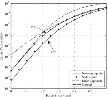
In Figure 2, we plot the error probability as a function of the rate withn= 60. Despite the fact that the block length is small, we observe that rcus and rcuc∗s are indistinguishable at all rates. Similarly, the gap from rcu to rcuc∗s is small. Consistent with the fact that Theorem 7 gives an asymptotic upper bound onrcu rather than an asymptotic equality,rcuc∗s
lies slightly above rcu at low rates. The error exponent approximation is close torcusat low rates, but it is pessimistic at high rates. The normal approximation behaves somewhat similarly to rcus, but it is less precise than the saddlepoint approximation, particularly at low rates.
To facilitate the computation ofrcuandrcusat larger block lengths, we consider the symmetric setup of δ0 =δ1 =δ2=
δ= 0.1andQ= 13,13,13
. Under these parameters, we have
I(X;Y) = 0.633 andRcr(Q) = 0.192 bits/use. In Figure 3, we plot the rate required for each random-coding bound and approximation to achieve a given error probability= 10−8, as a function ofn. Once again,rcucsis indistinguishable from rcus, and similarly for rcuc∗s and rcu. The error exponent approximation yields similar behavior torcus at small block lengths, but the gap widens at larger block lengths. The exact asymptotics approximations are accurate other than a divergence near the critical rate, which is to be expected from
4The plots remained the same when this value was increased or decreased by an order of magnitude.
0 0.1 0.2 0.3 0.4 0.5 10−8
10−7 10−6 10−5 10−4 10−3 10−2 10−1 100
Rate (bits/use)
E
rr
or
P
rob
ab
ili
ty
Non−asymptotic Saddlepoint Error Exponent Normal
rcus
rcu
Figure 2. i.i.d. random-coding bounds for the channel defined in (56) with minimum Hamming distance decoding. The parameters are n= 60,δ0 =
0.01,δ1= 0.05,δ2= 0.25andQ= (13,13,13).
100 200 300 400 500 600 700 800
0.05 0.1 0.15 0.2 0.25 0.3 0.35 0.4 0.45
Block Length
R
at
e
(b
it
s/u
se
)
Non−Asymptotic Saddlepoint Exact Asymptotics Error Exponent Normal rcus
rcu
Figure 3. Rate required to achieve a target error probabilityfor the channel defined in (56) with ML decoding. The parameters are= 10−8,δ
0=δ1= δ2=δ= 0.1andQ= (13,13,13).
the discussion in Section V-B. In contrast to similar plots with larger target error probabilities (e.g. [11, Fig. 8]), the normal approximation is inaccurate over a wide range of rates.
VI. DISCUSSION ANDCONCLUSION
We have introduced a cost-constrained ensemble with mul-tiple auxiliary costs which yields similar performance gains to constant-composition coding, while remaining applicable in the case of infinite or continuous alphabets. We have studied the number of auxiliary costs required to match the performance of the constant-composition ensemble, and shown
that the number can be reduced when the input distribution or decoding metric is optimized. Using the saddlepoint approxi-mation, refined asymptotic estimates have been given for the i.i.d. ensemble which unify the regimes of error exponents, second-order rates and moderate deviations, and provide ac-curate approximations of the random-coding bounds.
Extension to Channels with Input Constraints
Suppose that each codeword x is constrained to satisfy 1
n Pn
i=1c(xi) ≤ Γ for some (system) cost function c(·). The i.i.d. ensemble is no longer suitable, since in all non-trivial cases it has a positive probability of producing code-words which violate the constraint. On the other hand, the results for the constant-composition ensemble remain un-changed provided that Q itself satisfies the cost constraint, i.e.P
xQ(x)c(x)≤Γ.
For the cost-constrained ensemble, the extension is less trivial but still straightforward. The main change required is a modification of the definition of Dn in (19) to include a constraint on the quantity 1nPn
i=1c(xi). Unlike the auxiliary costs in (19), where the sample mean can be above or below the true mean, the system cost of each codeword is constrained to be less than or equal to its mean. That is, the additional constraint is given by
1
n
n X
i=1
c(xi)≤φc, X
x
Q(x)c(x), (136)
or similarly with both upper and lower bounds (e.g. −δ n ≤ 1
n Pn
i=1c(xi)−φc ≤ 0). Using this modified definition of Dn, one can prove the subexponential behavior of µn in Proposition 1 provided that Q is such that φc ≤ Γ, and the exponents and second-order rates for the cost-constrained ensemble remain valid under any such Q.
APPENDIX
A. Proof of Theorem 2
The proof is similar to that of Gallager for the constant-composition ensemble [15], so we omit some details. The codeword distribution in (18) can be written as
PX(x) =
1
µn n Y
i=1
Q(xi)11 ˆ
Px∈ Gn , (137) where Pˆx is the empirical distribution (type) of x, and Gn is the set of types corresponding to sequences x ∈ Dn (see (19)). We define the sets
Sn(Gn),PXY ∈ Pn(X × Y) : PX∈ Gn (138)
Tn(PXY,Gn),
e
PXY ∈ Pn(X × Y) : PeX ∈ Gn, e
We have from Theorem 1 that pe = rcu. . Expanding rcu in terms of types, we obtain
pe=. X
PXY∈Sn(Gn)
P(X,Y)∈Tn(PXY)
min
1,
(M −1) X
e
PXY∈Tn(PXY,Gn)
P(X,y)∈Tn(PeXY)
, (140)
wherey denotes an arbitrary sequence with typePY. From Proposition 1, the normalizing constant in (137) satisfies µn = 1. , and thus we can safely proceed from (140) as if the codeword distribution were PX =Qn. Using
the property of types in [15, Eq. (18)], it follows that the two probabilities in (140) behave as e−nD(PXYkQ×W) and
e−nD(PeXYkQ×PY) respectively. Combining this with the fact that the number of joint types is polynomial in n, we obtain
pe
.
=e−nEr,n(Q,R,Gn), where
Er,n(Q, R,Gn), min PXY∈Sn(Gn)
min
e
PXY∈Tn(PXY,Gn)
D(PXYkQ×W) +
D(PeXYkQ×PY)−R +
. (141) Using a simple continuity argument (e.g. see [28, Eq. (30)]), we can replace the minimizations over types by minimiza-tions over joint distribuminimiza-tions, and the constraints of the form
|EP[al(X)]−φl| ≤ nδ can be replaced by EP[al(X)] = φl. This concludes the proof.
B. Proof of Theorem 3
Throughout the proof, we make use of Fan’s mini-max theorem [41], which states that minasupbf(a, b) = supbminaf(a, b)provided that the minimum is over a com-pact set,f(·, b)is convex inafor allb, andf(a,·)is concave in b for all a. We make use of Lagrange duality [17] in a similar fashion to [5, Appendix A]; some details are omitted to avoid repetition with [5].
Using the identity[α]+= max
ρ∈[0,1]ραand Fan’s minimax theorem, the expression in (27) can be written as
Eccr (Q, R) = max ρ∈[0,1]
ˆ
E0cc(Q, ρ)−ρR, (142)
where
ˆ
E0cc(Q, ρ), min PXY∈S({al})
min
e
PXY∈T(PXY,{al})
D(PXYkQ×W) +ρD(PeXYkQ×PY). (143)
It remains to show thatEˆ0cc(Q, ρ) =E0cc(Q, ρ). We will show this by considering the minimizations in (143) one at a time. We can follow the steps of [5, Appendix A] to conclude that
min
e
PXY∈T(PXY,{al})
D(PeXYkQ×PY) = sup s≥0,{rl}
X
x,y
PXY(x, y) log
q(x, y)s P
xQ(x)q(x, y)se
P
lrl(al(x)−φl), (144)
wheresand{rl} are Lagrange multipliers. It follows that the inner minimization in (143) is equivalent to
min PXY∈S({al})
sup s≥0,{rl}
X
x,y
PXY(x, y) log
PXY(x, y)
Q(x)W(y|x)
+ρlog q(x, y) s P
xQ(x)q(x, y)se
P
lrl(al(x)−φl)
!
. (145) Since the objective is convex in PXY and jointly concave in (s,{rl}), we can apply Fan’s minimax theorem. Hence, we consider the minimization of the objective in (145) over
PXY ∈ S({al}) with s and {rl} fixed. Applying the tech-niques of [5, Appendix A] a second time, we conclude that this minimization has a dual form given by
sup {rl}
−logX x,y
PXY(x, y) P
xQ(x)q(x, y) seP
lrl(al(x)−φl)
q(x, y)seP
lrl(al(x)−φl)
!ρ
,
(146) where{rl} are Lagrange multipliers. The proof is concluded by taking the supremum oversand{rl}.
C. Necessary Conditions for the Optimal Parameters 1) Optimization of Ecc
0 (Q, ρ): We write the objective in (39) as
E0cc(Q, ρ, s, a),ρX
x
Q(x)a(x)−X x
Q(x) logf(x), (147) where
f(x),X y
W(y|x)q(x, y)−ρs
X
x
Q(x)q(x, y)sea(x)
ρ
.
(148) We have the partial derivatives
∂f(x)
∂Q(x0) =ρg(x, x
0) (149)
∂f(x)
∂a(x0) =ρQ(x
0)g(x, x0), (150)
where
g(x, x0),X y
W(y|x)q(x, y)−ρs
×ρ X
x
Q(x)q(x, y)sea(x)
!ρ−1
q(x0, y)sea(x0) (151) We proceed by analyzing the necessary Karush-Kuhn-Tucker (KKT) conditions [17] for(Q, a)to maximizeEcc
0 (Q, ρ, s, a). The KKT condition corresponding to the partial derivative with respect toa(x0)is
ρQ(x0)−X x
Q(x)ρQ(x
0)g(x, x0)
f(x) = 0, (152)
or equivalently
X
x
Q(x)g(x, x 0)