User Manual
analySIS
Imaging Solutions for Light Microscopy
Any copyrights relating to this manual shall belong to Olympus Soft Imaging Solutions GmbH. We at Olympus Soft Imaging Solutions GmbH have tried to make the information contained in this manual as accurate and reliable as possible. Nevertheless, Olympus Soft Imaging Solutions GmbH disclaims any warranty of any kind, whether expressed or implied, as to any matter whatsoever relating to this manual, including without limitation the merchantability or fitness for any particular purpose. Olympus Soft Imaging Solutions GmbH will from time to time revise the software described in this manual and reserves the right to make such changes without obligation to notify the purchaser. In no event shall Olympus Soft Imaging Solutions GmbH be liable for any indirect, special, incidental, or consequential damages arising out of
purchase or use of this manual or the information contained herein.
No part of this document may be reproduced or transmitted in any form or by any means, electronic or mechanical, for any purpose, without the prior written permission of
Olympus Soft Imaging Solutions GmbH.
Windows, Word, Excel and Access are trademarks of Microsoft Corporation which can be registered in various countries.Adobe and Acrobat are trademarks of Adobe Systems Incorporated which can be
registered in various countries.
© Olympus Soft Imaging Solutions GmbH All rights reserved
Printed in Germany ESbS51007
Olympus Soft Imaging Solutions GmbH, Johann-Krane-Weg 39, D-48149 Münster, Phone: (+49)251/79800-0, Fax: (+49)251/79800-6060
Contents
Step by Step analySIS ...5
Installing analySIS ...5
Any questions or problems? ...9
First Steps ...12
The (GUI) User Interface ...12
Loading images ...14
Displaying multiple images ...18
Saving GUI configuration ...21
Acquiring images ...25
Acquiring images using intX ...25
Configuring inputs ...26
Optimizing display ...30
Acquiring images ...34
Calibrating inputs ...37
Saving images ...41
Showing scale bar ...45
Saving / Printing / E-mailing ...48
Saving images ...48
Printing images ...50
E-mailing images ...53
Archiving images ...57
Define a database ...57
Define the directories for data storage ...57
Set up a new database ... 58
Define organizational fields ... 63
Define database fields... 63
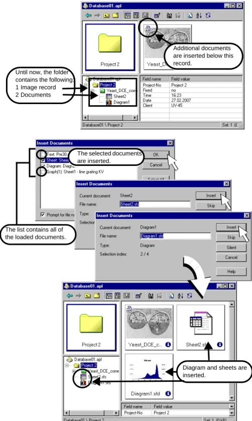
Insert data ...66
Create a new database folder ... 66
Insert images... 73
Insert documents... 73
Work in the database window ...81
Arrange fields ... 76
Choose view... 79
Find data ... 84
Load data ... 86
Archive data ...89
Protect with a password ...94
Processing images ...96
Editing overlay ...96
Increasing image contrast ...101
Adjusting image color ...103
Filtering gray-value images ...106
Interactive Image Measurement ...111
Save, load and edit measurement results ...113
Create measurement sheets ...116
Using statistics functions ...119
Measuring arbitrary structures ...120
Optimizing work environment for measuring ...124
Creating 3-D surfaces ...128
Creating models ...128 Editing models ...130 Coloring models ...133 Measuring models ...136Image Analysis ...139
Phase analysis ...139 Detecting particles ...141 Image preparation ... 142 Setting thresholds ... 145Defining detection area ... 147
Defining detection ... 150
Measuring particles ... 153
Editing detection interactively... 159
Classifying particles ... 161
Possible stumbling blocks during a particle analysis ... 166
Report Generator ...168
Creating reports ...168
Saving / Exporting report ...172
Report objects ...173 Image Objects ...177 Record objects ...181 Text objects...188 Sheet objects ...192 Diagram objects ...197 Report templates ...197
Creating / saving new templates ...197
Object templates ...202
Planning report templates ...204
Step by Step analySIS Step by Step analySIS - Background information
5
Step by Step analySIS
Installing analySIS
Background information
Welcome to analySIS!
The software package you have chosen is by Olympus Soft Imaging Solutions. You have thus entered into the worldwide analySIS-user community. Welcome. The broad range of functions for digital image acquisition, image processing, analysis, database archival and results documentation are all at your disposal in analySIS. We think you’ll find working with analySIS a tremendously satisfying experience!
analySIS configuration
analySIS is available in many various expansion versions and configurations. This means that some functions described in this "Step by Step" introductory manual, or in other documentation may not be included in the software package you have cho-sen - or vice versa - some functions that are included in your package may not be described below.
www. olympus-sis .com
Stop on by our website. It is chock full of information including: our ever-growing range of products, how to contact our customer service hotline, all about our upcom-ing workshops and seminars - and much much more.
Software protection The software is protected by a dongle. It is standard practice that a USB dongle, which is to be installed on one of your PC's USB ports, comes with the computer. For PCs that don't have a USB port, an LPT dongle is available on request.
The software is protected by a dongle. On the left you can see the LPT dongle for the parallel port on the right, the standard USB dongle.
•
analySIS can neither be installed nor started without the dongle.•
The dongles are differently colored, depending on which type they are:•
A network dongle can be connected to any of the computers of the network. Please keep in mind that before analySIS can be installed, the driver software for the network dongle has to be installed first. The Setup menu includes an op-tion for installing the driver software for the network dongle.USB-Dongle LPT-Dongle Meaning
blue white unlimited single license
black not
available
limited time dongle which only unlocks the software for a limited amount of time.
red red network dongle
Related topics
Step by Step analySIS Installing analySIS - Step-by-step
6
Step-by-step
Installing the analySIS software
1) Turn on your PC and, if necessary, start up the operating system.
2) Close any and all application programs.
3) Insert the software protection key (dongle) into a USB port of your PC.
"
The Found New Hardware Wizard dialog box will appear. The operating system will then try to install a driver for the dongle.As soon as you have in-serted the software pro-tection dongle, the Found New Hardware Wizard dialog box will appear.
4) Close the Found New Hardware Wizard dialog box by clicking the Cancel but-ton.
Keep clicking the Cancel button until the dialog box disappears.
5) Place the analySIS installation CD into the CD-ROM drive.
"
The setup program will start automatically - unless you have deactivated the autorun function. If so, start the setup.exe file manually via Windows Explorer.Warning Install the image analysis program before connecting the camera with the FireWire slot. This sequence is necessary to avoid having the operating sys-tem install the wrong camera driver. The camera drivers which are required for the operation of the cameras are installed together with the software.
Warning The installation of the hardware is described in the corresponding installation manu-al. The notes on hardware installation in this chapter apply solely to Olympus Soft Imaging Solutions' FireWire cameras.
Step by Step analySIS Installing analySIS - Step-by-step
7
When you insert the in-stallation CD the setup menu will come up automatically.
6) Select the analySIS FIVE option in the setup menu to install or update this soft-ware.
7) An installation wizard guides you through the entire software installation. Simply follow the onscreen instructions and select the relevant entries.
Update/Reinstall
•
Should you already have analySIS installed, Setup offers you an update of the installation. You should select this option to keep important program settings. These settings include the calibration data, for example.Precalibrated input channels
•
When working with a light microscope, the input channel can be precali-brated. This can, however, only be done with certain camera types such as the FireWire cameras from Olympus Soft Imaging Solutions, for example.Hardware
installation
•
analySIS supports different types of microscopes, stages and cameras. Select your hardware during installation so that the correct drivers are in-stalled.
"
After successful installation, a program file with the links to the installed components is opened.8) You may now connect your FireWire camera to your computer.
9) Doubleclick the program symbol to start the software.
•
The icon to start analySIS can be dragged and dropped onto your desktop while you press the [Ctrl] key. You can then conveniently open analySIS with one doubleclick.10) Doubleclick on the "Read Me" icon for the latest information on analySIS.
Related topics
Step by Step analySIS Installing analySIS - Step-by-step
8
Installing the network dongle
These step-by-step instructions are only relevant when you use a network dongle. In these instructions, "Server" stands for the computer on which the network dongle and the license manager have been installed.
"Client" stands for all computers which are part of the network and which must be connected to the server in order to install and operate an analySIS version.
1) First install the license manager on the server. The license manager is required for the operation of the network dongle.
2) Plug in the dongle on the computer which is to be the server and start the setup program from the analySIS CD.
3) Select the Network software protection key option in the setup menu.
4) In the Installation type dialog box select the Service option.
"
The license manager is installed after a few standard questions have been answered."
The installation of the dongle has then been completed. You don't have to install an analySIS version on the server."
You don't need to copy the license manager onto any client PC.To enable analySIS to locate the license manager more quickly
To make a quick and reliable access to the license manager possible, you should copy the "nethasp.ini" file onto every single client PC. The "nethasp.ini" file uses the server's IP address. How you find out this IP address, and how you use the "nethasp.ini" file will be described in the following.
Display the server's IP address
To find out the server's IP address, when using the Windows operating system, do the following.
1) Click the Windows Start button on the PC into which you've inserted the network dongle and installed the license manager on.
2) Select the Run... command.
3) Enter "Command" and confirm with OK.
4) Enter the command "ipconfig" in the command window and confirm with the [En-ter] key.
"
The IP address belonging to this computer will be shown in the command window.5) Copy the IP address you've found to your Windows clipboard. Inserting the
"nethasp.ini" file
1) Select the Explore this CD option in the analySIS setup menu.
You will find the "nethasp.ini" text file in the \program\HASP\Network\ Help di-rectory.
2) Make a backup copy of this file. Open the copy you've created.
3) Replace the entry "127.0.0.1" in this file with the contents of your Windows clip-board.
4) Save the modified file under the name "nethasp.ini".
"
In the modified "nethasp.ini" file, the IP address you found for your server will then appear on the "NH_SERVER_ADDR=" line.5) Copy the modified "nethasp.ini" file to the Windows directory (c:\winnt or c:\windows) of all of the PCs that have been installed in the network, on which analySIS versions run.
"
By employing this adapted "nethasp.ini" file, you make the search for the license manager in the complete network much easier. Starting analySIS on every single client PC will take place more quickly.Step by Step analySIS Any questions or problems? - Background information
9
Installing analySIS on the server
Is analySIS to run on the PC on which the license manager has also been installed, the following step will have to additionally be taken.
Copy the unmodified "nethasp.ini" file to the server's (c:\winnt or c:\windows) Windows directory. (You will find the "nethasp.ini" file in the \program\HASP\Net-work\ Help directory.
"
With the help of the "nethasp.ini" file, analySIS can then also be installed on the PC into which the network dongle has been inserted. In this file, the "127.0.0.1" entry is a reference to the PC itself.Installing PDF documentation
1) Select the Documentation option in the setup menu to have PDF documentation files copied onto your PC’s hard drive in full or in part.
2) Simply follow the onscreen instructions and select the documentation desired.
"
A program icon that looks like a book will appear within the program folder selected. This is a link to the documentation files that were just installed.3) Select the Quit option to exit the setup menu.
•
To start up analySIS and/or the documentation you had installed, simply doubleclick on the corresponding icon(s).•
Via the setup menu you can copy/delete additional parts of the documen-tation to/from your hard disk.Any questions or problems?
Background information
Other documentation
All documentation is also available as PDF files on the analySIS installation CD. To select the files you wish to have copied onto your hard drive, go to the setup menu. These files can be viewed onscreen and printed out using Acrobat Reader by Adobe (comes with analySIS).
Depending on the scope of your order, you will also have been supplied with other manuals, as well as these step-by-step instructions.
See more tips by using the ? > Welcome...
Step by Step analySIS
Any questions or problems? - Step-by-step
10
Step-by-step
We want to hear from you.
If you have any questions or any problems you’re having difficulty solving on your own - even after consulting the relevant documentation - then contact our customer service, preferably by e-mail. Our customer-service representatives will be more than happy to assist you.
1) Start your image analysis program.
2) Try and specify when and under what exact conditions the problem you’re hav-ing occurs.
•
Ideally, you should try and be able to reproduce the problem/error. This fa-cilitates our customer service finding the source of the problem, and thus, a solution.3) Make an exact note of any possible onscreen error messages involved.
•
Or simply make a "screenshot" of the message(s). All you need to do to get a snapshot of the active window is to press [Alt+Print]. This copies the ac-tive window to the Windows clipboard. Then you can easily include the copied window in an e-mail, by pressing [Ctrl+V].•
Oversized e-mails can lead to transmission difficulties. It is thus not advis-able to copy ‘screenshots’ of an entire onscreen view into an e-mail.4) With the ? > About... command, open the About dialog box.
"
The About dialog box tells you what expansion version you have, the build number and the serial number of your version, as well as the operating sys-tem being used.•
Please be sure and have all this information available when you contact our customer service.You can have the most important software data displayed by using the ? > About... command.
5) Now all you need to do is to write us an e-mail describing the problem you’re having as precisely as possible (incl. snapshots if applicable). Include the sys-tem information as well. Then send it to us at our customer-service e-mail ad-dress.
Step by Step analySIS Any questions or problems? - Step-by-step
11
•
The easiest, and most convenient, way to contact our customer service, is by using the automatic e-mail generation function.The ? > About... > System Info... > Send command will automatically gen-erate an e-mail form, which you can then send to us when you've added the relevant details of the problem you’re experiencing. Before sending it off to us, please read the notes in the e-mail window, concerning the infor-mation on your system, which will be sent to us via this e-mail.
Should you not be able to send an e-mail from your PC, use the ? > About... > System Info... > Save Info command to save the files, so that you can send the e-mail from another PC.
•
Please feel free to call us or fax us as well - at the following numbers. Tel.: (+ 49) 2 51 / 7 98 00-0Fax: (+ 49) 2 51 / 7 98 00-6060 The ? > About... >
Sys-tem Info... > Send com-mand opens the window with the automatically generated e-mail form you use to contact our customer service. All necessary system info is automatically includ-ed in this e-mail form. All you need to do is enter a precise description of the question/problem you’re having and then just click on Send (up-per-left button, e-mail-window button bar) to send it off to us.
First Steps
First Steps - Background information
12
First Steps
The (GUI) User Interface
Background information
GUI The graphical user interface influences the appearance of a program. It determines which menus there are, how the individual functions can be called up, how and where files, e.g., images, are displayed, and much more. This chapter describes the basic elements of GUI.
Please note: The Graphical User Interface (GUI) in your image analysis program is fully adaptable to meet your own specific requirements.
Menu bar Many commands are accessible via the relevant menus. You can configure the menu bar as needed. Use the Special > Define Menu Bar... command to add, alter or re-move menus as you wish.
Image buffer box Each image is allotted its own image buffer within your image analysis program. When you start up your image analysis program all available image buffers will be empty. While using the program they get filled - by loading or acquiring images, and by performing various image operations for altering the image such that a new image results. During any given work session, this means that many images are accessible simultaneously. Only one image buffer however, may be active at a time.
Active image buffer
•
The image in the active image buffer will always be displayed in the image win-dow independent of how many other images are being displayed.•
The active image buffer contains either the live image or an acquired image. Any interactive input or measurements are always applied to the active image buffer.Button bars Commands you use frequently are linked to a button providing you with quick and easy access to these functions. Please note, that there are many functions which are only accessible via a button bar, e.g., the functions required for editing an image overlay. Use the Special > Edit Button Bars... command to make button bars look and include what you want them to.
Viewport manager The viewport manager enables you to determine how images are displayed in the im-age window. Your are provided with many ways - no matter what the application - for displaying your images optimally onscreen. You can hide the viewport manager to create more room for other windows, for example: To do so, use the [Alt+1] key stroke.
Image manager The image manager contains numerous tabs. Click the different tabs to alter the ap-pearance of the image manager. The first two tabs List and Gallery are reserved for the administration of images.
The operands box is for:
•
determining source and destination image buffers used in image processing op-erations which alter the original image, e.g., inversion.•
linking images for certain image processing operations, e.g., addition of two im-ages.Use the image buffer box:
•
for an overview of the images loaded,•
for rapid access to image information, such as its size and image type,Related topics
First Steps The (GUI) User Interface - Background information
13
•
to activate image buffers. The icon area•
is for printing, archiving or saving images one at a time.You can hide the image manager to create more room for other windows, for exam-ple: To do so, use the [Alt+2] key stroke.
First Steps
Loading images - Background information
14
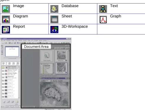
Document Area Documents can only be displayed within this area. Each document is opened within a separate window. Your image analysis program supports the following document types.
Image window The image window is a special window for viewing either loaded and/or live images. It is possible to view up to 25 images simultaneously. To display them, the image win-dow is divided up into several winwin-dows, i.e. viewports. Each viewport can display a single image.
To alter image display within the image window - e.g., zoom factor - use the Image
button bar.
Status bar The status bar displays the following and more:
•
brief descriptions of all functions. Simply move the pointer over the command or button for this information.•
name of the active input channel,•
position and size of the global frame.Loading images
Background information
Loading images You can load several images simultaneously. Click the Open button in the Open Im-age dialog box to load all selected image files. The image files will be loaded into suc-cessive image buffers. The first image buffer is the active image buffer.
To select...
•
a continuous group of images: Leftclick on the first of the images. Then, while pressing [Shift], leftclick on the last one of the images.Image Database Text
Diagram Sheet Graph
First Steps Loading images - Background information
15
•
a non-continuous group of images:Select the first image by clicking on it with the left mouse button. Keep the [Ctrl] key depressed as you select all image files needed with the left mouse button.
•
all images within a directory:Simply press [Ctrl+ A].
The File > Open... command is context-sensitive. This means the Open Image dialog box only appears if an image window is active. If a text document is active the Open Text dialog box will appear, etc.
The Open button is in the Standard button bar. To have a look at the dropdown list of all the various commands for opening, click the arrow beside this button.
Image-buffer-box icons
After you have loaded an image, it will be displayed in the image manager. Image type, image name and resolution are directly displayed in the image manager. The displayed information are somewhat different depending on whether or not you have set the list or gallery view in the image manager.
A resolution of 318 x 223 x 24 corresponds to a true-color image with a bit depth of 24, width of 318 pixels and a height of 223 pixels. The gallery view shows you thumbnails in the image-buffer box of all images currently loaded (right).
Possible image types are: Empty image buffer
A gray value image can be comprised of 256 (8 Bit) or 216 (16 Bit) gray values.
A binary image is comprised of 2 gray values - black and white.
A false-color image is an 8-bit gray-value image whose gray-values are shown in color.
A true-color image, or RGB image, is comprised of 224 colors (24-bit).
A Fourier image is a 32-bit image made up of real and imaginary numbers of 16 bits respectively.
First Steps
Loading images - Step-by-step
16
Step-by-step
Loading images stored on the hard drive
1) Click on the image buffer you wish to load the image into with the left mouse button in the Image Manager. Activate - for example - image buffer #5.
"
The image buffer selected will be color highlighted and assigned to the ac-tive viewport.2) Select the File > Open... command to load an image.
"
The Open Image dialog box will appear. Dialog boxes for loadingfiles are based on stan-dard MS Windows dia-log boxes. The diadia-log box for loading images also has a preview func-tion.
3) Select Tagged Image Format (*.tif), the standard image format, in the Files of type list.
•
This format is the default when you open this dialog box for the first time. The Files of type list is inall dialog boxes for load-ing documents. It pro-vides file formats for all document types.
4) Click the Up One Level button to move up a level in the directory structure of your computer.
"
In the field below the button bar you will find a list of all sub-folders and doc-uments of the file types selected.5) Doubleclick on one of the folders listed to get a listing of its contents - i.e., all sub-directories and files the folder contains.
•
The root directory of your program contains the "Images" sub-directory. A selection of TIF images is available here.6) Click the Preview button to view thumbnails of image files. Select the image files one at a time.
First Steps Loading images - Step-by-step
17
8) Click the Open button to load the images selected.
"
The Open Image dialog box will be closed."
The images will be loaded into successive image buffers. The first image will be loaded into the active image buffer, e.g., #5. The next images you load are then put into image buffers 6-9 (if you have loaded altogether 5 images simultaneously).Activate image window
Sometimes the image window is covered by another window. This is the case if a document window has been maximized or if many other documents are open. The following step by step instruction is only one possibility to bring the image window back to the foreground.
1) Select the Window > Document-Manager... command or use the [Alt+3] key stroke.
"
You will find all of the open document windows listed in the document man-ager. The document type and the title of the document window are given for each document.2) Select the image window.
"
There is always one image window!3) Click the Activate button located in the document manager.
"
The image window is now in the foreground.Loading images into specific image buffers 1) Click the Gallery tab in the image manager.
2) Activate the image window by simply leftclicking within the window.
•
If the header of the Images window is in color, this means it is active.3) Select the Standard (button bar) > Open... command.
4) Leftclick on the image file you wish to load.
5) Drag the file directly onto any one of the image buffers while pressing the left mouse button (drag&drop).
"
The image buffer will show a preview of the image you have loaded.6) Repeat the last step as often as needed.
First Steps
Displaying multiple images - Background information
18
Use the mouse to drag&drop images into the image buffer de-sired. MS Explorer, a file man-ager, can also be used for drag&drop loading.
Displaying multiple images
Background information
Viewport A viewport is a window in the image window where each of the loaded images, or the live image is displayed. You can divide the image window into numerous viewports, thus displaying numerous images simultaneously.
The viewport manager enables you to influence the way images are dis-played in the image win-dow.
The viewport manager has a separate button bar for setting viewport properties fast.
Button Description
Arrange View-ports
Determines the amount and order of the viewports in the image window.
Display Proper-ties
Opens the Display Properties dialog box. Enables you, for example, to change the ap-pearance of the viewports and the maximum amount of viewports.
You can enter a comment for each image which is then saved together with the image. Use the display properties to show this image comment in the viewport.
The Display-Properties > Visualization tab enables you to select a false color view for all loaded gray-value images.
Zoom This button enables you to increase or decrease the size of the image in the active viewport by increments of 100%.
First Steps Displaying multiple images - Step-by-step
19
Select one of the 3 pos-sible views from the viewport manager:
Dual Screen System
This paragraph is only relevant if your system supports two monitors. A dual screen system means that there is an additional monitor which is exclusively used for view-ing images. The Windows monitor is the main monitor on which your operatview-ing sys-tem runs. The second monitor is called the dual monitor. The dual monitor solely con-tains an additional image window.
The viewport manager contains a tab for each monitor. Click on the appropriate tab to switch back and forth between the monitors. Use the buttons located in the view-port manager, to influence the appearance of the dual monitor.
Step-by-step
Optimizing display
1) Press [Ctrl+Alt+T] to generate a test image.
•
The image window contains a button bar with which you can quickly alter the appearance of the images in the image window.Display Configu-ration
This button enables you to save all viewport settings. You can also link images with viewport settings which can be loaded together with the viewport settings.
Select Viewport Manager Pane
You see a schematic monitor in the viewport manager. This button enables you to de-termine what is to be shown in this monitor. Three views are possible:
View Viewports The viewport view is the default view. It shows you the current order of the viewports in the image window. In other words, you see the image window in a schematic view. The image names and numbers of the image buffers are shown in the image buffer instead of the images. You will need this view when working with dual screen systems. Navigator The navigator view shows the image in the active image buffer. The image is
com-pletely shown in the navigator. You can define the image section which is shown in the image window directly in the overview image located in the navigator.
Rightclick in the viewport manager to open the context menu. Select the Show Live
command to view the live image in the navigator.
Magnifier The magnifier shows a magnified portion of the image in the active image buffer. Move the pointer across the image. The shown section always corresponds to the image sec-tion which is directly under the pointer. Rightclick in the viewpoint manager to set the zoom factor of the magnified image.
First Steps
Displaying multiple images - Step-by-step
20
Press [Ctrl+Alt+T] to generate a test image. It will have a color image overlay which displays current monitor resolu-tion and other informa-tion. Press [Ctrl+Alt+Shift+T] to generate a color test im-age. The test image is auto-matically the same size as the active viewport. The test image will al-ways be displayed at 100% zoom. The header shows the number of the image’s image buffer, (2), the image name, (Test), and the current zoom factor (100%).
2) Click the Arrange Viewports button to re-define the number and arrangement of viewports. Select a 1x2 arrangement.
"
The image window will be divided up into two viewports. The test image is in the left viewport. Image buffers will be reassigned. Zoom factors will be set to Auto. Though reduced in size somewhat, the entire test image will be shown.3) Click the Single View button to display just one image in the image window - the active viewport image.
"
The viewport arrangement and what image buffers are shown in which viewports remain unchanged.4) Select one of the entries of the Zoom Factor dropdown list - or enter any zoom factor desired into the field directly; e.g., 30%.
"
The test image will be reduced to 30% zoom. The viewport will no longer be totally taken up by the image. Where the patterned background starts (in the viewport) is where the image stops.5) Click the Zoom In button to double the current zoom factor.
"
The test image will now be displayed at a zoom factor of 60%.6) Click the Adjust Zoom button to have the zoom factor adjusted to fit current viewport size.
•
The length/width ratio of the image will not change. Unlike the automatic zoom factor, this zoom factor is not linked to the size of a window - i.e., even when you adjust the size of a window, the zoom factor stays the same.7) Alter the size of the image window.
8) Click the Adjust Window button to have window size adjusted to fit current im-age size.
9) Click the Zoom button in the viewport manager.
"
You will now see a magnifying glass appear in the active viewport. Use the mouse to move it. As soon as the magnifying glass touches the top border of the viewport, the image will be moved upward.First Steps Saving GUI configuration - Background information
21
•
Leftclick to raise the zoom factor by 100%, e.g., from 300% to 400%. Rightclick to lower the zoom factor by 100%, e.g., from 300% to 200%. The minimum zoom factor is 100%.Click the middle mouse button (or press [Esc]) to exit the zoom mode.
10) Click the Select Viewport Manager Pane button located in the viewport manag-er. Select the Navigator view. Select what image segment you want shown (in the image window) within the thumbnail.
•
Move the mouse onto the red-frame border around the thumbnail. The mouse pointer will change shape, turning into a double arrowhead. While pressing the left mouse button you can reduce the frame in size. The length/width ratio of the frame will be the same as the viewport in the image window.•
Now move the mouse to within the red frame. The mouse pointer will now turn into a four-pronged arrowhead. You can move the frame by moving the mouse while pressing the left mouse button."
The image segment you selected will be shown in the image window.11) Magnify the images zoom factor, so that only one image section is shown in the image window. Use the slide control located in the image window to move the image section.
"
The frame in the navigator moves accordingly and once again shows the current image position.Within the thumbnail in the viewport manager you can define which image segment is to be displayed within the im-age window. To define the segment, adjust the size of the frame and move it to where you want it within the Navi-gator.
Saving GUI configuration
Background information
Workspace You can save your graphical user interface in a file. This is called a workspace. A workspace includes the layout of all document windows and button bars as well as how viewport and image manager are positioned. It can also include specific images and documents you wish to have loaded.
First Steps
Saving GUI configuration - Background information
22
•
Defining GUI layoutYou may want to define workspaces for each of the various kinds of tasks, thus optimizing how the graphical user interface is laid out for each of these. Sepa-rate workspaces could be for image acquisition, report generation and image analysis. Having separate workspaces gets you the onscreen layout you need and fast.
•
Reloading images/documentsThe path names of currently loaded images and documents can be saved in a workspace. Saving the current GUI in a workspace at the end of your workday makes it totally easy for you to continue where you left off the next morning. Any and all images, sheets, diagrams, database(s), report(s) that were loaded when you saved the workspace will be right where you left them.
Configuration versus Workspace
The Special > Configuration command enables you to individually determine ele-ments on your user interface, as well. Please note that the configuration and work-space contain different elements of the user interface. Configuration refers to what commands have been defined for menus, button bars and keyboard, e.g., user-de-fined button bars. A configuration saves what functions are available on your GUI. A workspace, however, actually saves what the GUI looks like, including specific doc-uments. The information saved in workspaces and configurations is totally different. The program interface can greatly differ in appearance. In the example below, the image graphs, sheets and database windows are arranged so that they do not cover each other. This order is optimal when wanting to do intensity profiles or measure his-tograms. You can save such a layout in a workspace.
Please not that there is a default workspace for working with reports. Use the [Ctrl+2] key stroke to load this workspace.
Warning Be sure to save all your images before shutting down your image analysis program. Any unsaved images will be deleted without prior warning.
First Steps Saving GUI configuration - Step-by-step
23
Step-by-step
Saving GUI layouts as workspaces
1) Open documents of all the types you wish to have included in your graphical user interface (GUI), e.g., an image, a database, a measurement sheet and a diagram. Close all other documents.
Use the Measure > Histogram... command to quickly create a diagram and sheet in addition to the active image.
•
Press [Alt+1] and [Alt+2] to make both viewport and image manager disap-pear from view.2) Arrange the windows optimally to your satisfaction within the GUI.
•
Select the Special > Preferences > View > Allow tiling and cascading of im-age window check box. Then select the Window > Tile Vertical menu com-mand.3) Select the File > Workspace > Save as.... command.
•
Enter a name for your workspace into the File name field of the Save Work-space dialog box, e.g., "analysis".•
Disable the Load documents (not only layout) check box so that only the layout of the GUI is saved, and not any specific documents.•
Select the Do not save option to ensure this workspace remains un-changed when you close it.First Steps
Saving GUI configuration - Step-by-step
24
Loading workspaces
1) Activate the Workspace button bar. This is done by selecting the following check box: Special > Edit Button Bars... > Button bars > Workspace.
"
This button bar has 5 buttons which represent 5 workspaces. The first two buttons are already assigned to the predefined workspaces called "nor-mal" and "report". The third button represents the new workspace you have just defined ("analysis").•
To make any changes as to what workspaces the buttons represent, sim-ply use the File > Workspace > Define Menu... command.2) Let’s have a look at how a workspace can be used: First, load a different work-space: e.g., the predefined workspace called "normal". Simply click on the but-ton for this workspace (the first one) to load it.
3) Close all documents.
4) Now load your own user-defined workspace ("analysis"). Simply click the third button in the Workspace button bar.
5) Then load an image, your database, a sheet and a histogram. All these docu-ments will be positioned according to your workspace layout.
Creating workspaces to use day-in and day-out
1) Select the File > Workspace > Save as... command. In the dialog box, enter the name of the workspace, e.g., date. Select the Load documents check box. Se-lect the Confirm save on close option. Close the dialog box.
"
The fourth button now represents this workspace.•
At the end of your workday: save all images you wish to retain. Any images that have not been saved will be deleted without any prior warning and are thus lost for good.Close down your image analysis program. Click Yes when a message ap-pears asking you whether or not you wish to save this workspace. All doc-uments that have not been saved will result in similar messages. Save those documents you wish to hang onto.
The next time you start up all those documents will be loaded automatically as well.
Acquiring images Acquiring images - Background information
25
Acquiring images
Your image analysis program supports a wide array of cameras and acquisition de-vices. The commands for acquisition depend on the acquisition devices or cameras being used. The functionality can therefore diverge considerably from what is de-scribed here. Divergences occur between a digital camera or a video camera, for ex-ample.
Acquiring images using intX
Background information
intX The abbreviation intX stands for intelligent Exposure. Use this acquisition process to make good acquisitions with functions that are easy to use. The intX acquisition pro-cess is only offered for cameras made by Olympus Soft Imaging Solutions.
Image resolution: acquisition and snapshots
A considerable advantage of using intX is that you can select different resolutions for the live-image (acquisition) and for the snapshot. A lower image resolution is sug-gested by default for the live-image since the frame rate is then higher and thus the movements in the live-image are not choppy. If you are writing a snapshot to the im-age buffer, it is recommended, however, to select the highest camera resolution pos-sible in order to attain the optimal in image quality.
intX enables you to automate the acquisition process to a large extent. The exposure times for live acquisitions and snapshots are optimized independently of one anoth-er. The optimization of the exposure time occurs continually and automatically.
Camera calibration Before you can use intX for the first time, your image analysis program has to cali-brate the camera. This calibration is solely required to determine your camera's spe-cial properties, which are required for the automatic calculation of the exposure times. To carry out this calibration, simply follow the directions your image analysis program gives you.
XY-calibration and intX
intX uses the calibration data of the active input channel for the XY-calibration of the images.
intelligent Exposure of-fers a convenient alter-native to the acquisition commands Images > Acquisition and Images > Snapshot.
Click the left mouse but-ton to start the live-im-age. Click the right mouse button to end the live-image and to write the image to the image buffer.
Warning Illustrations and examples in the following chapter are based on the CCD color camera ColorViewIIIu.
Related topics
Acquiring images
Configuring inputs - Step-by-step
26
Step-by-step
Acquire images using intX
This command is not available for all cameras and software configurations.
1) Select the Images > intelligent Exposure... command.
"
The intelligent Exposure dialog box is opened. When using this dialog box, you still retain access to all of your image analysis program's other func-tions.2) Should this be your first time using intX, you will receive the message that your camera has not yet been calibrated. Follow the directions.
3) Click the Acquisition button to begin the live-acquisition.
"
The exposure times calculated by intelligent Exposure are displayed in the dialog box's status bar. The term Live Exp. (Live Exposure Time) stands for the exposure time of the live acquisition, while Snap Exp. (Snapshot Ex-posure Time) stands for the exEx-posure time of the snapshot. Independent of the calculated exposure time for the snapshot, the exposure time for the live acquisition cannot exceed 125 ms. In this way, a quickly reacting live-image is guaranteed, which simplifies setting the microscope while the camera is running.4) Bring the image into focus.
•
Before you focus, click the Focus mode button. By doing this you will switch the camera to the highest resolution. One camera pixel is then ex-actly equal to one pixel on your screen. Then click the Focus mode button once more to return to a view of the complete image.5) Click the White Balance button to conduct a white balance. In the image win-dow, move the ROI's red rectangle to a white or uniformly gray position on the specimen. Change the size of the ROI by keeping the mouse depressed and moving the mouse. Rightclick to confirm position and size of the ROI.
•
When using a reflected light microscope, you can simply take a white sheet of paper as a sample for the white balance.When using a transmitted light microscope, try to find a position on the mi-croscope slide without a sample.
6) The Exposure adjustment slide control enables you to manually influence the exposure time for snapshots as calculated by intelligent Exposure. Move the
Exposure adjustment slide control to the right to increase the exposure time, or to the left to shorten it.
7) Click the Snapshot button to acquire a single image.
"
intelligent Exposure acquires a snapshot and writes it to the active image buffer. The snapshot acquisition ends the live mode.Configuring inputs
Background information
Logical input channel
Your image analysis program uses the concept of logical input channels when ac-quiring images via camera, slowscan-interface, or other acquisition devices. A logical input channel includes all settings relevant to image acquisition. The graphical user interface of a logical input channel is basically the same for physically-different
ac-Acquiring images Configuring inputs - Step-by-step
27
quisition devices - such as digital cameras or video cameras. The only differences are in the available functions in the Configure Input dialog box and the Camera con-trol.
Usually, the setup program installs the appropriate input channel so that you can start acquiring images immediately after installation. You only then have to configure the input channel when you want to use special camera settings. In the input channel you can, among other things, set the following aquisition parameters:
•
the image resolution,•
calibration data,•
live-image display within viewport,•
real time functions such as the live-overlay or an over exposure warning and•
macro commands to be carried out either before or after image acquisition. You can, for example, select the microscope magnification before the acquisi-tion or have a scale bar automatically drawn into the image after the acquisiacquisi-tion.Online shading correction
Optical systems consisting of camera and microscope generate image inhomogene-ity, or so called shading, even if care was taken with setting up the devices. The shading makes itself noticed by the fact that the image gets darker toward the edge. A shading correction corrects these image flaws with the help of reference images. Using the online shading correction of ColorViewIIIu these corrections already take place in the live-image.
The online shading correction is activated in the logical input channel. Before the on-line shading correction is able to be used, you must acquire these reference images. In addition to the camera characteristics, the microscope's optical characteristics, es-pecially the objective being used, contribute to the correction image. A correction im-age for each camera resolution and objective combination must be made according-ly.
A software wizard will guide you step-by-step through the acquisition of these refer-ence images. This wizard is automatically called up when you acquire the first image with the online shading correction activated.
Step-by-step
Set up a new input
Only set up a new input if no input has been predefined for your camera. Should an input already exist, it is usually better to duplicate the already existing input.
1) Select the Image > Set Input... command.
"
All current logical input channels are listed in the Set Input dialog box. You may duplicate an existing channel and then modify it, or set up an entirely new input channel.2) Click the New Channel button.
"
The Select Device dialog box will be opened.You will find predefined inputs for all image signals which can currently be read with your image analysis program.
3) Select the device desired in the Available devices list.
•
To display all inputs available, click on the plus sign (within the tree control directory).Acquiring images
Configuring inputs - Step-by-step
28
Two different system modes are offered for the ColorViewIIIu, Col-or and Black/White. In order to be able to use the Black/White mode, you must create a new channel.
4) Select, for example, "ColorView IIIu FW #...", if you have installed a CCD-color camera of the ColorViewIIIu type. The abbreviation "FW" stands for FireWire.
•
Two channels will be automatically set up for ColorView I and ColorViewIIIu. The channel with the additional "BW" must be used for the camera's black & white mode.5) Click on OK.
"
A new logical input will be added to the list of available input channels.6) Click the Configure Input button to define the properties of this input channel.
7) Close the two dialog boxes by clicking OK.
Duplicate already existing input
If you want to configure the input differently, first duplicate one of the already existing inputs. In doing so, you retain all of the channels settings.
1) Select the Image > Set Input... command.
"
All current logical input channels are listed in the Set Input dialog box.2) Choose one of the existing inputs, for example the ColorView IIIu FW input, if you have installed a CCD-color camera of the type ColorViewIIIu.
3) Click the Duplicate channel button.
"
The selected input channel is copied together with its settings and a new input channel is set up with these settings. The number 1 is added to the name of the input.Configure inputs
1) Select the Image > Set Input... command. Select an already existing input.
2) Click the Configure Input button to define the properties of this input channel.
"
The Configure Input dialog box will be opened. Doubleclicking on thecamera icon in the sta-tus bar will open up the Configure Inputdialog box also.
3) Click on the Info tab to change the name of the input channel.
4) Click on the Input tab to set image acquisition parameters.
•
The functionality of this tab will depend on what kind of camera you are us-ing. This may mean that your Input tab is significantly different to the one described here.Acquiring images Configuring inputs - Step-by-step
29
5) You do not have to make an entry in the exposure time field when configuring the input.
•
Exposure time may be interactively adjusted while viewing a live image. To do this, use the Camera Control dialog box (Image > Camera Control...command) during live-image acquisition.
•
The Sharpen filter may be activated/deactivated in this tab as well via the respective check boxes. Or, use the Camera Control dialog box to do the same thing - conveniently - during live-image acquisition. If you are using intX, the settings for the sharpen filter are adopted from the active input.•
The Camera field shows a description of your camera type. Click the Info...button for more information on the camera, for example the current tem-perature of the CCD chip and of the camera housing.
6) Select a predefined camera resolution from the Resolution list. The selected resolution influences the spatial resolution of the acquired images.
•
Please note: the larger the spatial resolution, the slower the camera works in live mode, and the longer the exposure times you'll need, will be. There-fore, it can make sense to define two channels with different resolutions. You still use the channel with the smaller resolution mainly for the live mode, whereas the channel with the larger resolution will be used for the snapshot image acquisition.7) Select the Online Shading-Correction > Activate check box to utilize the online shading correction.
Select the procedure used by you from the Illumination method list.
•
The online shading correction will immediately be used should correction images already exist for the current settings. Should no appropriate correc-tion images be available, your image analysis program will automatically start a software wizard for the acquisition of correction images.8) Click OK to close the dialog box. Logical input channel
properties will be de-fined in a single dialog box on several tabs. For every different camera configuration used you may define a separate input channel. Your im-age analysis program supports up to 100 channels. Scanners and cameras with a TWAIN interface may be operated via these input channels as well. New Channel Duplicate Channels Configure Input Delete Channel Configure Device Help Set Input
Acquiring images
Optimizing display - Background information
30
Optimizing display
Background information
Configure Input > Display
The Configure Input > Displaytab provides you with a number of possibilities for op-timizing the way live-images and snapshots are displayed on your screen. These in-clude:
•
having an overexposure warning appear;•
enhanced-contrast onscreen display of images even if acquisition conditions are poor, via automatic or fixed-scale contrast enhancement (Automatic gain display or Fixed scaling),•
checking on current intensity distribution (intensity = mean of all 3 color chan-nels) during image acquisition using the online histogram;•
activating live overlay;•
setting the scaling of an image within its viewport.N e w Chan nel Con figure Input > Inpu t
Acquiring images Optimizing display - Background information
31
Live overlay If the Live overlay check box has been selected, image overlays are also available to you in the live acquisition mode. This means you may:
•
conduct numerous measurements within a live-image as well and have the re-sults written in the overlay;•
have a measurement grid and automatic scale bar shown within the live image;•
during the live acquisition, already highlight and label image details (or more generally, write texts or insert graphics into the overlay).Please note: The following functions for Olympus Soft Imaging Solutions cameras are available only if the Live-Overlay has been activated: setting the ROI for white balance in the live-image, Partial Readout, and setting the ROI for a sharpness monitor in the live-image.
Automatic gain display
Use the automatic gain display to acquire images independent of the illumination pa-rameters. The system analyze the current histogram in real time and spreads the his-togram onto the entire dynamic range of the camera.
Even when working with the automatic gain display, you should align the exposure time with the actual illumination parameters. Use the online histogram as a check. The exposure time should be set in such a way, so that the spread of the histogram is as wide as possible, thus filling the entire dynamic range.
Please note: The automatic gain display only slightly improves the image contrasts. Over exposure cannot be corrected by the Automatic Gain DisplayInversely, there is increased noise if the image is very much underexposed.
You cannot use the Automatic Gain Display if you want to compare the intensities of numerous images with one another.
Acquiring images
Optimizing display - Background information
32
This online histogram shows a narrow distribu-tion. The image would thus be dark and lacking contrast without auto-matic gain display. When the Automatic Gain Display has been activated, the existing signal range will be spread to improve mon-itor display. This makes image structures much more clearly visible.
Online histogram If the Online-Histogram check box has been selected, you can check the intensity distribution during image acquisition. During image acquisition, a window showing the current histogram will appear automatically. This histogram will be continually up-dated.
The histogram shows you if the image is illumi-nated properly. The dis-tribution is cut-off to the right if the image is over-exposed. If the image is underexposed, the dis-tribution shows a peak at the left.
Image scaling Your image analysis program offers you several possibilities to customize the size of the image to fit the active viewport. The view of the image in the viewport does not have any effect on the actual image resolution.
•
Underscan: the system automatically selects from the zoom factors (of 25%, 50%, 100%) the one at which the entire image is displayed within the viewport. This may mean that some viewport space is left over.•
Overscan: the system automatically selects from the zoom factors (of 25%, 50%, 100%) the lowest zoom factor at which the complete viewport is taken up by the image. In certain cases, the image will not be visible in its entirety.•
Adjust to viewport: image size is adjusted to fit the viewport’s current size. In some cases, stripes can appear in the live-image display. Should this be the case, use either the Underscan scaling or the Overscan scaling.•
Full size (100%): the live-image will be shown with no zoom factor. If the port is smaller than the image, only as much of the image as fits within the view-port will be shown.Acquiring images Optimizing display - Step-by-step
33
Depending on the im-age scaling selected, the image will appear in different sizes in the viewport.
Step-by-step
Optimize live display
1) Select the Image > Configure Input... command (or click on the Configure Input
button in the Set Input dialog box).
2) Select the Display tab.
3) Select the Display warning check box in the Over exposure group.
4) Enter 0.5 into the Overflow field.
"
The program will then caution you, "Warning! Over exposure!" as soon as more than 0,5% of the image's pixels are white, during an acquisition.5) Select the Activate check box in the Automatic gain display group.
"
Now the image will always be shown with enhanced contrast onscreen no matter what the actual illumination conditions are. Please note that over-exposure and/or over illumination cannot be corrected by the automatic gain display.6) Enter the value 0.01 in the Right overflow field.
"
Now 0.01% of the brightest image pixels will be displayed white onscreen.•
Use the right overflow value to prevent pixels which are too bright from in-terfering with the automatic gain display.•
A Left overflow value cannot be defined for the ColorViewIIIu.7) Select the Online Histogram check box to check the actual intensity distribution during a live image acquisition and to appropriately adapt the exposure time. (Intensity = mean value of the three color channels).
"
The histogram will appear during live image acquisition automatically."
In addition, the minimum, mean and maximum intensity values of the cur-rent image will be shown. The percentages refer to the camera's maximum possible value. For a 12-bit camera this value is 4095; for an 8-bit camera 255.Acquiring images
Acquiring images - Background information
34
8) Select the Live overlay check box to be able to write information into the image overlay during live acquisition.
The live overlay is also a necessary requirement for some of the other functions, e.g., partial readout, which you can activate in the camera controls.
9) Select one of four display options in the Image scaling list.
10) Confirm the settings you have made by clicking OK.
Acquiring images
Background information
Live-acqui-sition mode
In the live-acquisition mode you see the live-image in the active viewport. The re-quirements for the live acquisition are determined by the active input channel. Use the live-acquisition mode for focusing, illuminating and positioning your specimen un-der the microscope. While in the live-image mode, only those commands that are rel-evant in this mode are available to you.
Acquiring snapshots
Selecting the Image > Snapshot command acquires a single image via the active log-ical input channel and places it in the active image buffer. Use this command to quit the live-acquisition mode as well.
When an image is acquired, additional image information is also saved; e.g., calibra-tion data and current input magnificacalibra-tion. Rightclick on an image buffer to access any of this image information via the context-sensitive menu.
Camera control
Camera control gives you quick and easy access to the most important camera set-tings - and interactively during live acquisition, too.
The functions available in the Camera Control dialog box will depend on what kind of camera you’re using. When us-ing a ColorView IIIu the dialog box appears as below:
Exposure time determines for what length of time the camera's CCD chip is to be illuminated. -/+ alters the value in pseudologarithmic steps. Auto sets the value after the automatic evaluation of the current histogram during a live-image.
Please note: The image area is the basis of the calculation which you also deter-mine for the automatic gain display. When acquiring images with extreme contrasts, you should not use the automatic exposure time. Fluorescence images, for exam-ple, are very quickly overexposed when you use it.
Color settings opens a dialog box containing slide controls which enable you to correct color errors and with which you can set the gamma values and the color saturation.
White balance corrects a tinge - either in the live-image or in the snapshot.
Use the button with the red frame to define the image area which is to be used to calculate the white balance.
Sharpen Filter On/Off
activates / deactivates the sharpness filter, which makes the image sharper or softer, depending on the sharpness filter settings.
Acquiring images Acquiring images - Background information
35
Sharpen Filter Settings
opens the dialog box containing the slide control for the sharpen filter. Maximum values are -30 (soft) and +30 (sharp). The value 0 makes the filter have no effect. Use automatic
gain display
activates / deactivates the automatic contrast enhancement. Now the image will al-ways be shown with enhanced contrast onscreen no matter what the actual illumi-nation conditions are.
Histogram-cal-culation on en-tire image
All of the pixels are used for calculating the current histogram.
This histogram is evaluated for the automatic contrast enhancement. In addition, the histogram determines the automatic exposure time, which you can access by clicking the Auto button located in the camera controls.
... cross-hairs Only pixels of a horizontal and vertical line (each one pixel in diameter) located in the center of the image are included in the histogram's calculation.
... ROI Only the pixels within a frame set by you (Region Of Interest) are included in the calculation of the current histogram.
Set ROI sets a red frame into the image which you position with the mouse and whose size you can increase or decrease by keeping your left mouse button depressed. The right mouse button enables you to set the frame which then becomes invisible. Use fixed
scal-ing
activates/deactivates the fixed scaling contrast enhancement. It works with fixed limits, unlike the automatic contrast enhancement which evaluates the currently up-dated histogram.
Fixed Scaling ... ... automatic set-ting
automatically recalculates the fixed limits for the current camera settings.
... manual setting opens the dialog box in which you can redefine the fixed limits for the fixed scaling contrast enhancement.
Black balance corrects the image background. The program calculates the mean value for each color channel in an area (ROI) which you defined. These values are subtracted from all pixels in the entire image. The black balance is to be used predominately for flu-orescence acquisitions in order to balance the undesired background in the acquisi-tion.
Please note: Do not use the black balance with brightfield acquisitions. If you did, you would change the colors in the images.
Use the button with the red frame to define the image area which is to be used for the black balance.
Sharpness Moni-tor On/Off
shows/hides the sharpness monitor. The sharpness monitor consists of a dialog box in which a relative measurement of the sharpness is displayed by a changing bar which can vary between "Blurred" and "Focused". In doing so, the green bar shows the maximum sharpness reached since the live acquisition was started. The black line shows the minimum sharpness reached so far.
Use the button with the red frame to define the image area which is to be used for calculating the image sharpness.
Partial Readout enables quick live acquisitions. A rectangular part of the image is defined for the partial readout to which the readout is limited during the live acquisition. A higher frame rate is attained due to the smaller amount of data being transferred. The live overlay must be enabled for the partial readout. The live overlay can be en-abled via the Display tab located in the Configure Input dialog box.
Use the button with the red frame to define the area of the image which is to be read out.