ABSTRACT
Fluid catalytic cracking (FCC) process is a vital refinery process which majorly produces gasoline. In this research, a hybrid algorithm which was constituted of Adaptive Neuro-Fuzzy Inference System (ANFIS) and firefly optimization algorithm was developed to model the process and optimize the operating conditions. To conduct the research, industrial data of Abadan refinery FCC process were carefully gathered along a definite period. Then a model based on ANFIS was developed to investigate the effect of operating variables including reactor temperature, feed flow rate, temperature of top of main column, and the temperature of bottom of the debutanizer tower on quality and quantity of gasoline, LPG flow rate, and process conversion. Moreover, statistical parameters comprising R2, RMSE, and MRE approved the accuracy of the model. Eventually, validated ANFIS model and firefly algorithm as an evolutionary optimization algorithm were applied to optimize the operating conditions. Also, three different optimization cases including maximization of Research Octane Number (RON) , gasoline flow rate, and conversion were considered. In addition, to obtain maximum target output variables, inlet reactor temperature, temperature of top of main column, temperature of the bottom of debutanizer column, and feed flow rate should be respectively set at 523, 138, 183 °C and 40731 bbl/day. Also, the sensitivity analysis between the input and output variables was carried out to derive some effective rules of thumb to facilitate operation of the process under unsteady state conditions. Finally, the obtained result introduces a methodology to compensate for the negative effect of undesirable variation of some of the operating variables by manipulating the others. Keywords: Fluid Catalytic Cracking, Adaptive Neuro-Fuzzy Inference System, Firefly Algorithm, Optimization, RON, Gasoline.
*Sorood Zahedi Abghari
Research Group of Modeling and Control Process, Process Development Engineering, RIPI, Tehran, Iran
Sensitivity Analysis and Development of a Set of Rules to Operate FCC
Process by Application of a Hybrid Model of ANFIS and Firefly Algorithm
*Corresponding author Sorood Zahedi Abghari Email: [email protected] Tel: +98 21 4825 5107 Fax: +98 21 4473 9712
Article history
Received: January 16, 2018
Received in revised form: November 23, 2018 Accepted: December 8, 2018
Available online: August 7, 2019
INTRODUCTION
For over fifty years, Fluid Catalytic Cracking (FCC) has been one of the main petroleum refining processes to produce gasoline. This is designed to process wide range of feed stock including straight run distillates, atmospheric and vacuum residue,
it is transferred to the regenerator to burn off the coke. Same as other chemical processes like catalytic reforming process [1], isomerization [2], hydrodesulfurization, [3] and thermal cracking [4], modeling and simulation are directly applied in a FCC process to monitor the performance, optimize the operating variables, and control the process [5-12,23-26]. Kinetic models with different lumps were utilized or developed to estimate the effect of different designing or operating variables on the conversion of a FCC process or to develop dynamic models to control the process [5-11], or it is used to optimize the quality of produced gasoline [12]. Since the kinetic models are complex, the convergence rate of the developed process model based on these kinds of models is low. So for some applications, other kinds of modeling methods such as black box modeling are utilized. Moreover, this becomes more significant for complex processes such as thermal cracking, FCC process, and food industrial processes [13,24-28]. For example, an artificial neural network (ANN) was applied to investigate the steady state of a FCC process located in a Greek refinery complex. In this research, a comparison between the developed model and a regression model approved that the developed intelligent model was more precise in comparison with the regression model [27]. Also, ANFIS was applied to investigate the hydrocracking process [28]. For example, ANFIS was applied to investigate the hydrocracking process [28]. In the research, sixteen data sets were gathered along a definite period. Moreover, thirteen set of data were applied to train the model, and the rest were utilized to check the validity of the developed model [28]. Catalyst-life as one of the most important parameters in the processes with catalytic fixed
optimization algorithm to determine suitable operating conditions. Moreover, the results will apply to figure out certain rules to compensate the negative effects of the variation of operating variables in different situations.
EXPERIMENTAL PROCEDURES
Specification of the FCC Process
The feedstock of the process is vacuum gasoil (VGO) with the characterization demonstrated in Table 1. The selected FCC process, is a process which is licensed by UOP, and it has high-efficiency regenerator technology. Before feeding to the process, the feed is preheated to 232 °C to improve the conversion of the process. Then it is injected to the riser-reactor in which the feed is vaporized due to close proximity to a hot catalyst. The catalytic cracking exothermic reactions have occurred in the effective volume of riser-reactor while the catalyst over oil ratio is between 4 and 9. In addition to main products, the coke is also produced and formed on catalyst. It is removed by burning later in regenerator. The catalyst and product mixtures are separated in cyclones.
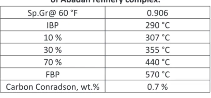
Table 1:The characterization of the feedstock of FCC of Abadan refinery complex.
Sp.Gr@ 60 °F 0.906
IBP 290 °C
10 % 307 °C
30 % 355 °C
70 % 440 °C
FBP 570 °C
Carbon Conradson, wt.% 0.7 %
The products are sent to the separation section of the process and the catalyst is sent to the regenerator to reactivate and coke removal. Selected FCC unit processes 45000 bbl VGO to produce LPG, HCO, LCO, and gasoline. In addition maximum flow rate of produced gasoline is four
million liters per day. Specification of the utilized catalyst is illustrated in Table 2.
Table 2: Fresh FCC catalyst characteristics used in the FCC process of Abadan refinery complex.
Apparent bulk density, g/mL 0.7-0.9 Total Surface area, m2/g 130-370
Micropore surface area, m2/g 100-250
Mesopore Surface area, m2/g 30-120
Rare earth content, wt.% Re2O3 None For Low micropore Surface Area 0.3-1.5 For high micropore surface area 0.8-3.5 Alumina, wt.% Al2O3 25-50
MATERIAL AND METHODS
Field Data
been selected as validated data. The upper and lower limits of the observed value of the chosen input variables and the maximum and minimum observed value of the output variables are illustrated in Table 3.
Table 3: Upper and lower limits of chosen input, and maximum and minimum observed value of output variables of FCC process of Abadan Refinery Complex.
Operating variable Lower limit Upper limit
Feed flow rate (bbl/day) 40000 43000
Reactor Temperature (°C) 519 525
TBDC (°C) 169 184
TTMC ( °C) 133 139
Output variable Minimum Value Maximum Value
Gasoline flow rate (bpd) 20580 22600
LPG flow rate (bpd) 8293 8720
RON 92.8 94
Conversion (%) 68.7 70.65
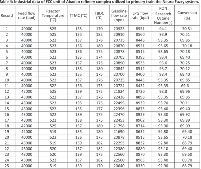
Table 4: Industrial data of FCC unit of Abadan refinery complex utilized to primary train the Neuro Fuzzy system.
Record Feed flow rate (bpd) Temperature Reactor
(°C) TTMC (°C)
TBDC (°C)
Gasoline flow rate
(bpd)
LPG flow rate (bpd)
RON Research
Octane Number(-)
Conversion (%)
1 40000 525 135 170 20923 8551 94.1 70.51
2 40000 525 135 182 20910 8560 93.9 70.51
3 40000 522 137 176 20735 8446 93.35 69.85
4 40000 523 136 180 20870 8521 93.65 70.18
5 40000 523 136 175 20878 8515 93.65 70.18
6 40000 522 135 174 20705 8395 93.4 69.40
7 40000 523 137 175 20890 8535 93.6 70.25
8 40000 523 135 180 20842 8512 93.7 70.12
9 40000 522 135 175 20700 8400 93.4 69.40
10 40000 522 137 176 20735 8445 93.35 69.85
11 40000 522 136 175 20724 8432 93.35 69.6
12 42000 525 139 175 21824 8720 93.8 69.96
13 43000 522 137 176 22436 8898 93.35 69.85
14 43000 523 135 175 22499 8939 93.70 70.11
15 43000 522 135 177 22396 8875 93.40 69.40
16 43000 522 139 175 22470 8929 93.30 69.92
17 43000 522 138 175 22453 8902 93.30 69.89
18 42000 525 137 180 21798 8714 93.90 69.09
19 42000 519 135 180 21690 8632 92.80 69.40
20 40000 523 136 175 20878 8515 93.65 70.18
21 43000 519 139 182 22255 8832 92.80 68.79
22 43000 520 137 182 22380 8880 93.10 69.40
23 43000 520 139 175 22560 8870 93.30 69.50
24 43000 522 137 182 22560 8965 93.40 69.70
25 40000 519 139 170 20640 8330 92.90 68.79
MATHEMATICAL METHODOLOGY
ANFIS Architecture
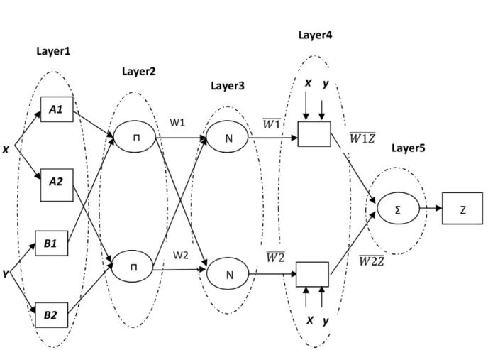
A fuzzy logic and ANN combination is utilized in Neuro-Fuzzy technology. Indeed, learning capabilities of neural networks with knowledge representation of fuzzy logic results in the development of adaptive Neuro-Fuzzy inference system (ANFIS). Moreover, the Neuro-Fuzzy model is based on the Takagi-Sugeno type fuzzy inference system with a single output. This model utilizes a linear combination of the input parameters to predict the output of each rule. The structure of an ANFIS with two inputs (x and y) and one output (z)
is shown in Figure 1.
If a first-order Sugeno fuzzy model is assumed for a system with two inputs and one output, a common set of rules is written as below:
Rule 1: if x is A1, and y is B1, then Z1= P1x+q1y+r1. (1) Rule 2: if x is A2, and y is B2, then Z2=P2x+q2y+r2. (2) As it is illustrated in Figure 1, the Neuro-Fuzzy system contains a total of five layers. Moreover, the nodes of each layer have the following functions: Layer 1: every node in this layer is an adaptive node with the following node function:
Q1,i = μA,i(x) ; i=1,2 or (3) Q1,i= μB,i-2(x) ; i=3,4 (4)
where x and y are the inputs to the first node, and Ai and Bi-2 are the fuzzy set that is associated with the node. A “fuzzy set” is a simple extension of the definition of a classical set, in which the characteristic function is permitted to have any value between 0 and 1. In addition, a “fuzzy set” A of X can be defined as a set of ordered pairs: A={(x,μA(x)|xεX} (5) where μA(x), which is a membership function for the fuzzy set A, maps each x to a membership grade between 0 and 1.
Determination of the optimal type and number of the membership functions is the primary step in the development of the fuzzy inference system. The most popular membership functions include the triangular, Gaussian, generalized bell, and trapezoidal functions, which are defined as follows (Equations 6 to 9):
0
− −
= − −
x a c x
triangle(x;a,b,c) max min( , ),
b a c b (6)
Gaussian(x;σ,c)=exp (x c2 2)2
−
−
(7)
( )
( )2
1 ; , , 1 = − + b
bell x a b c
x c a
(8)
(9)
in which a, b, c, d, and б are the fundamental parameters of the membership functions. Layer 2: Nodes in this layer are fixed and have the label Π. Based on Equation 10, the outputs of nodes are the products of all of the incoming signals which represent the firing strength of a fuzzy rule. O2,i = wi = μAi(x) * μBi (x), i =1,2 (10) Layer 3: Every node in this layer is also fixed and is labeled as N. The ratio of the firing strength of the rule relative to the sum of the firing strengths is calculated by the ith node:
σ
(11)
The layer outputs are known as “normalized firing strength.”
Layer 4: every node (i) in this layer is an adaptive node with a node function that is defined as the following:
(12) where wi is a normalized firing strength from layer 3 and {pi, qi, ri} is the parameter set of the node. The parameters in this layer are called “consequent parameters”.
Layer 5: The single node in this layer is a fixed node and is labeled Σ. This calculates the overall output as the summation of all of the incoming signals.
1 5, 1 1 = = = =
∑
=∑
∑
n n i i ii i i n
i i i
w z
O w z
w (13)
Thus an adaptive network, which is functionally equivalent to the Takagi–Sugeno-type fuzzy inference system, was constructed. Based on the ANFIS structure described, the output z can be defined as the following:
1 2
1 2
1 2 1 2
= +
+ +
w w
z z z
w w w w
(14) In which p1, p2, q1, q2, r1, and r2 are the linear consequent parameters.
A hybrid learning procedure was used to train the proposed ANFIS model, which includes the tuning of the premise parameters using a back propagation technique and the learning of the consequence parameters by the least-square method. This hybrid learning algorithm is composed of two phases. The first is a forward pass in which the node outputs are passed forward until they reach layer 4, and the consequent parameters are calculated through least squares. The second phase is a backward pass in which the error rates are propagated backward,
(
)
(
)
1 1 1 1 2 2 2 2
=w p x q y r+ + +w p x q y r+ +
1 0
− −
= − −
x a d x
trapozoid(x;a,b,c,d) max min( , , ),
b a d c
3 1 2 1 2 = = = + ( ,i)
O i , ,
i '
w
w i
w w
(
)
4,i= i i = i i + i + i , =1 2,
and the gradient descent technique is used to update the premise parameters.
The accuracy of the developed Neuro-Fuzzy model is appraised using statistical parameters including the coefficient of determination (R2), the root mean square error (RMSE), and the mean relative error (MRE). The parameters are calculated by the following equations:
(
)
(
)
2 2 1 2 1 1 = = − = − −∑
∑
n expi cali i n expi exp i y y Ry y (15)
(
)
1
1
=
=
∑
n expi− calii
RMSE y y
n (16)
1
1 − 100
=
=
∑
calin expi y
i expi
y
MRE *
n y (17) where yexp and ycal are respectively the experimental and model-predicted values. Also,yexp illustrates
the mean of experimental values. However “n” is the total number of data points. To determine the best structure of targeted ANFIS model, different Neuro-Fuzzy models with different numbers of membership functions were checked. Finally, it was revealed that a combination of two Gaussian functions introduce the best shape of the membership function for most precise model. In this model, the linguistic labels were chosen to represent the input parameters. In addition, values of the statistical parameters for the model in the case of train and test are illustrated in Table 4. The developed ANFIS model has fifty five (55) nodes. The number of linear parameters is eighty (80) and the number of non-linear parameters is twenty four (24).
Optimization
Optimization of the operating conditions for achieving a certain goal is always the subject of several types of research in the field of the chemical
process. It may include profits maximization, limitation of the production of undesirable products, and optimum production of a strategic product. In the current work, RON maximization, gasoline production flow rate, and conversion are the three different optimization goals. Firefly algorithm as a metaheuristic nature-inspired algorithm is applied to attain the optimum operating conditions. Moreover, this algorithm is based on the social (flashing) behavior of fireflies or lighting bugs in the summer sky in the tropical regions. It has three exact idealized rules which are based on some of major flashing characteristics of real fireflies [33]. These are as follows: (1) all fireflies are assumed as unisex; the fireflies move towards more attractive and brighter ones regardless of their sex. (2) The amount of attraction of a firefly is proportional to the brightness of the fireflies. It decreases by increasing the firefly distance from others, regarding to the fact that the air absorbs the light. However, the brightest ones move randomly. (3) The brightness or lighting power of a firefly is established by the value of the objective function of a given problem. In addition, to apply this algorithm a computer code that is published by Xin-She Yang, has been utilized [33]. Following equations are introduced to obtain maximum RON, gasoline production flow rate, and conversion by minimizing the difference between the actual and the maximum value of the variables:
Constraints
The constraints indicate the limitations of operating conditions which are determined based on the authentic process. Equation f(1) shows the objective function to minimize the difference between the maximum obtainable and actual RON. Likewise, f(2) indicates the minimization of the difference between the maximum obtainable and actual conversion. Moreover, equation f(3) introduces an objective function to minimize the difference between the actual and maximum possible gasoline production flow rate.
519≤Reactor Temperature≤525
4 4
4 10x ≤Feedflowrate≤4.3 10x
133≤Temperature of Top of Main Column≤139
168≤Temperature of Bottom of Debutanizer Column≤184
RESULTS AND DISCUSSION
Industrial data were collected from the FCC process during the eighteen-month period. The validated industrial data were divided into three groups to be applied in training, test, and validation of the developed ANFIS model. The results of statistical tests and estimation of statistical parameters (R2 and MRE) for the data are illustrated in Table 4. Moreover, the scatter diagrams plotted from the ANFIS model prediction for gasoline flow rate, RON, LPG flow rate, and conversion are given in Figure 2 (a, b, c, and d). In addition, the same type of plots for CO, LCO, and lean gas flow rate are given in Figure 3 (a, b, and c).
Figure 3: Scatter diagrams for the accuracy of the ANFIS model (Validation case) for prediction of: (a) CO production flow rate (bbl/day), (b) LCO production flow rate (bbl/day), and (c) lean gas production flow rate.
Based on Table 4, Figures 2 and 3, it would be suggested that the developed ANFIS model prediction have enough accuracy to predict the output variables. However, the LCO prediction model has the lowest precision. Indeed, the LCO prediction model has the lowest precision, and the gasoline production flow rate has the highest accuracy.
Table 5: Statistical results of Neuro-Fuzzy model for prediction of gasoline flow rate, RON, conversion and
LPG flow rate.
Statistical
parameter Gasoline flow rate RON LPG flow rate CO LCO Lean Gas
R2(Train) 0.98 0.94 0.93 0.925 0.91 0.95
MRE
(Train) 0.41 0.35 0.72 1.31 2.51 1.05
R2 (Test) 0.958 0.927 0.905 0.912 0.902 0.929
MRE
(Test) 2.78 3.25 4.02 3.45 4.25 3.85
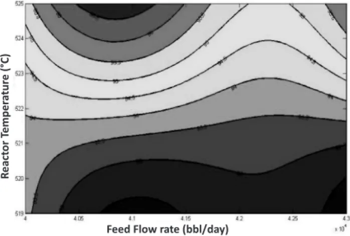
By applying the verified ANFIS model, the effects of different operating variables and their interactions on output variables are clarified. The main effects and the interactions of two major operating variables including feed flow rate and inlet reactor temperature on the gasoline production flow rate are elucidated by exploration of Figure 4. Raising the feed flow rate at a stable inlet reactor temperature increases the gasoline production rate.
Figure 4: Effects of reactor temperature (°C) and feed flow rate (bbl/day) on gasoline production flow rate (bbl/day).
CO (bbl/da
y) (Model)
CO (bbl/day) (Exprimental)
LC
O (bbl/da
y) (Model)
LCO (bbl/day) (Exprimental)
Lean Gas (bbl/da
y) (Model)
Lean Gas (bbl/day) (Experimental)
React
or T
emper
atur
e (
°C)
Indeed, in the operating range, definite rising in the feed flow rate yields almost the same increment in the gasoline production rate. In fact, 75 bbl/day increments in the feed flow rate would increase the gasoline flow rate by 62 bbl/day.
Moreover, the minor contribution of the inlet reactor temperature in the gasoline flow rate is related to the negligible effects of rates of reactions on the gasoline production flow rate.
Indeed, the maximum effect of reactor temperature is recorded while the feed flow rate is low and less than 4.05*104 bbl/day. However, by increasing the feed flow rate, the effect of reactor temperature is weakened. Eventually, the interaction effects of these two parameters can also be inferred from Figure 4. Indeed, increment in feed flow rate accompanying increase or decrease of the reactor temperature increases the gasoline production flow rate. However, decreasing the feed flow rate declines the gasoline flow rate, without considering the decrease or increase in the trend of the reactor temperature. The effect of TTMC and its interaction effect with reactor temperature on gasoline flow rate are illustrated in Figure 5.
Figure 5: Effects of reactor temperatures (°C) and TTMC (°C) on gasoline flow rate (bbl/day).
It is suggested that increasing the TTMC decline the gasoline flow rate by 4.65%. This is due to the fact that increasing the TTMC increases the escape
Figure 6: Effects of TBDC (°C) and Reactor Temperature (°C) on the gasoline flow rate (bbl/day).
chance of the heavier components from heavy products to the gasoline stream. In addition, the simultaneous increase in both variables increases the gasoline production rate ultimately by 7%. However, different variations in TTMC and inlet reactor temperature prove that the inlet reactor temperature has a prime effect on the gasoline flow rate in comparison with TTMC. Also, the study suggests that the maximum influence of reactor temperature on the gasoline flow rate happen at lower TTMC. In addition, the effect of reactor temperature is weakened at the medium operating temperature range.
Moving on, the main and the interaction effects of TBDC and reactor temperature on the gasoline flow rate are given in Figure 6. It is well demonstrated that at the specified feed flow rate and TTMC, increasing the TBDC decreases the gasoline flow rate by 13.3 %. In addition, this observation can be related to vaporization of some species of gasoline by increasing the TBDC.
The effects of reactor temperature and feed flow rate on RON are illustrated in Figure 7. As a whole, an increase in the inlet reactor temperature raises the RON. This figure (Figure 7) declares that increasing the reactor temperature increases the
React
or T
emper
atur
e (
°C)
Temperature of top main Column ( °C)
React
or T
emper
atur
e (
°C)
Figure 7: The Effect of reactor temperature (°C) and feed flow rate (bbl/day) on RON.
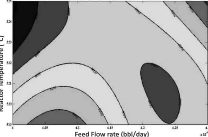
The main effect of TTMC and its interaction with reactor temperature on RON are demonstrated in Figure 8. The contour plot in Figure 8 contains two definite regions, i.e. the first region with a low reactor temperature, and the second region with high reactor temperature.
Figure 8: The Effect of reactor temperature (°C) and temperature-of-top-of-main-column (°C) on RON. Also, increasing the TTMC raises the RON in the former while in the latter, increasing the TTMC decreases the RON. Moreover, in the first region of the contour, increasing the TTMC will boost the ratio of high octane components in the gasoline product. However, in the high reactor temperature region the gasoline product contains enough species to supply the RON, increasing the TTMC can vaporize and recycle the components with a lower RON in the gasoline stream. Consequently, the RON is hindered by increasing the TTMC. By making a comparison among the variations of RON, TTMC, and reactor temperature, it is proved that the reactor temperature has the predominant effect. Indeed, increasing the reactor temperature by 1 °C will result in increasing one RON unit. However, 1 °C TTMC will ultimately improve the RON by half of a RON unit. The impact of reactor temperature is related to the decisive effect of this operating variable on the chemical reactions rate [34]. The influence of input variables on LPG production rate is demonstrated in Figure 9. Moreover, raising feed flow rate and inlet reactor temperature increases the LPG flow rate. Increasing the feed flow rate at low reactor temperature (less than 522 °C) generates special trends in the LPG production flow rate variation.
RON by 4.32 %. However, raising the feed flow rate would slightly decrease the RON. This is rationalized by the direct effect of reactor temperature on the reaction network [34]. Generally, increasing the temperature accelerates the rate of reactions. However, it may also accelerate both desired and undesired reactions. On the contrary, increasing the feed flow rate decreases the residence time of a reactive mixture in the reactor. Eventually, it decreases the chance of completion of reactions. In the operating range at low feed flow rates and temperature, increments in the feed flow rates decrease the formation of components which boost the RON. On the other hand, at a higher range of reactor temperature, increasing the feed flow rate decreases the formation of undesired products (secondary reactions). This consequently leads to a slight increase in a RON rating.
Feed Flow rate (bbl/day)
React
or T
emper
atur
e (
°C)
React
or T
emper
atur
e (
°C)
At first, increasing the feed flow rate increases the LPG flow rate. After reaching a maximum value, further increments in the feed flow rate decreases the LPG flow rate. However, at higher reactor temperature (more than 522 °C), increasing the feed flow rate increases the LPG production rate. This special trend can also be related to the interaction of residence time and reactor temperature on the reaction rate. Moreover, the amount of feed flow rate affects the number of products.
Figure 9: The impact of reactor temperature (°C) and feed flow rate (bbl/day) on LPG production flow rate(bbl/day). In Figure 10, the effect of feed flow rate and reactor temperature on total produced cycle oil (LCO and HCO) is demonstrated. The figure (Figure 10) illustrates that at low feed flow rates and high reactor temperature, the maximum cycle oil is observed.
Figure 10: The effect of reactor temperature (°C) and feed flow rate (bbl/day) on formation of total cycle oil (bbl/day) (LCO and HCO).
By making a comparison among Figures 4, 9, and 10, it is proved that at low feed flow rates and high reactor temperature, both the maximum flow rate of cycle oil and the minimum amount of LPG and gasoline are observed. However, at a higher reactor temperature and feed flow rates, the maximum LPG and gasoline flow rates are observed. Moreover, at this level, the cycle oil production rate is at the medium level. This clarifies the relationship among the products and their dependence on the operating variables. At high reactor temperature and low feed flow rates, the reaction network tends to produce heavy molecules. However, by decreasing the residence time (increasing the feed flow rates), the reaction network shifts to produce more light products while the reactor temperature raises the rates of all reactions. The effect of feed flow rate and reactor temperature on total FCC conversion is demonstrated in Figure 11. Thus it is reported herewith that the conversion of a process is minimized when the process operates at low reactor temperature and low feed flow rate. However, an increase in reactor temperature boosts the process conversion because it accelerates the rate of reactions. But, increasing the feed flow rate decreases the impact of temperature rising, since it decreases the residence time of a reactive mixture in the reactor.
Figure 11: The effect of reactor temperature (°C) and feed flow rate (bbl/day) on process conversion(%).
Feed Flow rate (bbl/day)
React
or T
emper
atur
e (
°C)
Feed Flow rate (bbl/day)
React
or T
emper
atur
e (
°C)
Reac
tor T
emper
atur
e (
°C)
The impact of TTMC and its interaction effect with reactor temperature are provided by the plot in Figure 12. The figure illustrates that the maximum conversion is observed at the maximum temperature and minimum TTMC. However, at a low reactor temperature of less than 522 °C, increasing the TTMC increases the process conversion. On the other hand, at a higher reactor temperature of more than 523 °C, increasing the TTMC decreases the process conversion. Furthermore, by having a medium reactor temperature range of 522 °C – 523 °C, increasing the TTMC has not any strong visible effects on the conversion of the process.
Figure 12: The effect of Reactor temperature and TTMC on process conversion.
Up until now, it has been shown that the sensitivity analysis presented here has facilitated in scrutinizing the results generated from the developed ANFIS model. Subsequently, the model was validated,
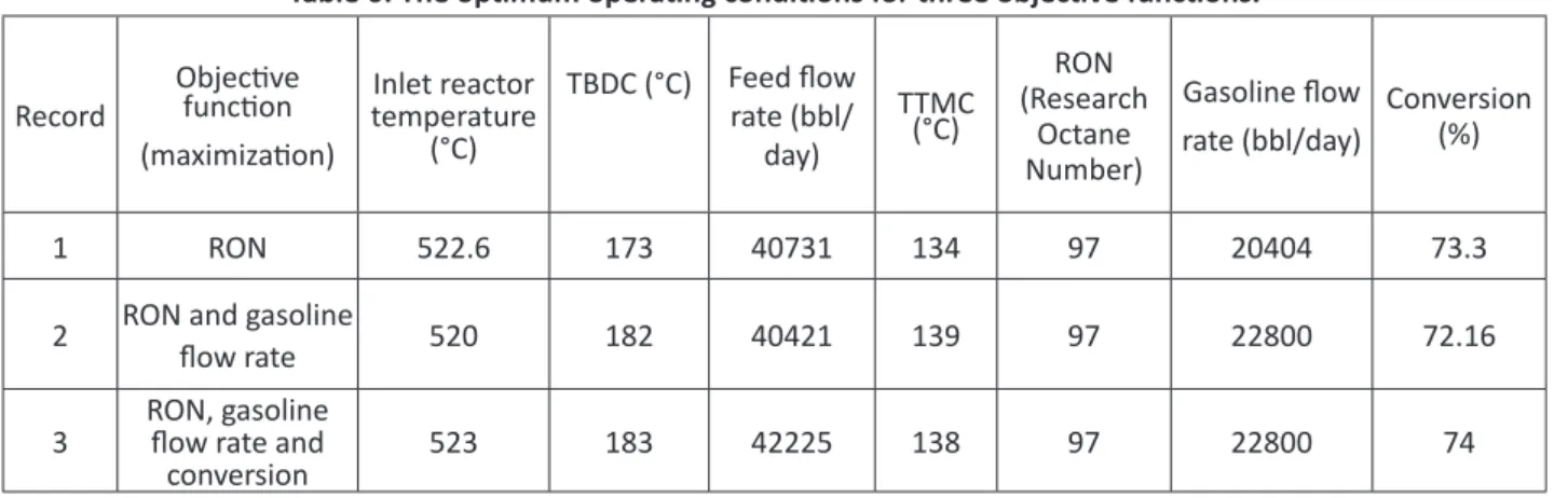
Table 6: The optimum operating conditions for three objective functions.
Record Objective function (maximization)
Inlet reactor temperature
(°C)
TBDC (°C) Feed flow rate (bbl/
day)
TTMC (°C)
RON (Research
Octane Number)
Gasoline flow rate (bbl/day)
Conversion (%)
1 RON 522.6 173 40731 134 97 20404 73.3
2 RON and gasoline flow rate 520 182 40421 139 97 22800 72.16
3 RON, gasoline flow rate and
conversion 523 183 42225 138 97 22800 74
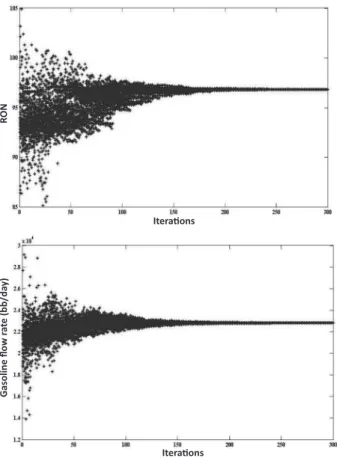
and it can be applied to investigate the optimum operating conditions. Firefly algorithm was further applied to minimize the objective function introduced by equation (1). Table 6 introduces the optimum operating conditions in three different cases. The three objective functions in Table 6 are respectively maximization of RON, of both RON and gasoline flow rate and of RON, gasoline flow rate, and conversion. From this table, it is thus reported herewith by us that maximization of all three selected output variables has occurred at the following optimum conditions viz (i) inlet reactor temperature = 523 °C, (ii) TBDC = 183 °C, (iii) feed flow rate = 42225 (bbl/day), and (iv) TTMC = 138.0 °C. However, when the goal of optimization is maximization of RON, the following optimized conditions are suggested as follows: (i) inlet reactor temperature = 523 °C, (ii) TBDC = 173 °C, (iii) feed flow rate = 40731 (bbl/day), and (iv) TTMC = 134.0 °C. The behavior of the firefly optimization algorithm is illustrated by Figure 13. The figure shows the plot of RON and gasoline production rate versus iterations of the firefly algorithm as it approaches optimum conditions. Figure 13 also shows that the maximum divergence of the sample population is observed in the first few tens of iterations. However, a rapid decline of the divergence is observed upon
Temperature of top main Column ( °C)
React
or T
emper
atur
e (
Figure 13: Plots of (a) RON and (b) gasoline production rate versus the iterations generated by Firefly algorithm.
Iterations
RO
N
Iterations
Gasoline flo
w r
at
e (bb/da
y)
CONCLUSIONS
Investigation towards process optimization of fluid catalytic cracking (FCC) – a vital refinery process which majorly produces gasoline - can be studied by analyzing the different range of available collected industrial data. The selected output variables were respectively gasoline, LPG, LCO, gas and CO production flow rates. However, these output variables are dependent on other so-called input variables, namely the inlet reactor temperature, feed flow rate, TTMC and TBDC which are recognized as the most effective ones.
In addition, an ANFIS model system was developed and trained by the industrial data gathered from
the FCC process of Abadan refinery complex. The industrial data were gathered during eighteen months, and 208 of the gathered industrial data were validated and selected for the model development. The validated data were divided into three sections, to be applied in training, test, and validation of the ANFIS model. The developed ANFIS model has fifty five (55) nodes. The number of linear parameters of the model is eighty (80), and the number of nonlinear parameters is twenty four (24). The results from the model validation confirmed sufficient accuracy.
The sensitivity analysis between the input and output variables was carried out by further exploiting the validated model data. Indeed, the sensitivity analysis clarifies the main and interaction effect of the operating variables. In addition, it is resulted in a set of rules to properly operate a FCC process with the high efficiency regenerator technology in different situations. It is shown that, the reactor temperature has a strong effect on RON, gasoline flow rate, LPG production flow rate, and even process conversion. The sensitivity analysis also illustrated that at high residence time and high reactor temperature, the production rate of heavy species was predominant and the amounts of light hydrocarbons were in minority.
Furthermore, in the light of this condition, the maximum RON may be obtainable. However, at high reactor temperature and low residence time, the maximum of light hydrocarbons including LPG and gasoline are observed. Moreover, at the specified conditions, the cycle oil production rate is at the medium level. The observation demonstrates that prolonging the residence time assists in the formation of heavy species components including the cycle oils. In addition, maximization of RON at high residence time and high reactor temperature improving the iterations until they converge to an
may be related to the fact that some of heavy species components including aromatic hydrocarbons have a tremendous impact on RON.
In addition to the above facts, certain guidelines could be formed based on the sensitivity analysis. The guidelines may be applicable to a FCC operational process in anomalous conditions. First of all, the effects of decreasing the feed flow rate on gasoline production rate could be partly compensated by raising the inlet reactor temperature. Averagely, changing 1 °C in reactor temperature could balance the effect of 300 bbl/day variation in feed flow rate. Moreover, RON, being the most important qualitative parameter of gasoline, is majorly affected by temperature. However, at the temperature higher than 523 °C, its dependence on the feed flow rate is becoming increasingly more. Indeed, within this temperature region, an increment of more than 500 lb/hr in the feed flow rate may change the RON if the reactor temperature has never been modified properly. Last but not least, in order to determine the optimum conditions for different objective functions as defined in this study, the firefly optimization algorithm was applied. The three alternatives, i.e. (i) RON, (ii) RON and gasoline flow rate, and (iii) RON, Gasoline flow rate, and conversion were analyzed and maximized. It was shown that maximization of RON, gasoline flow rate and conversion may be realized when the feed flow rate, inlet reactor temperature, TTMC, and TBDC set at 42225 bbl/day, 523 °C, 138 °C, and 183 °C respectively. The results of this research can be applied to facilitate operating determinations in a different situation such as abnormal states to compensate for the negative effect of some variation of operating variables. Also, the well trained ANFIS model can be implemented in the development of a robust MPC system.
ACKNOWLEGMENTS
The financial support provided by the Research and Development Center of Abadan Oil Refinery Complex is greatly appreciated.
NOMENCLATURES
ANN : Artificial Neural Network FCC : Fluid Catalytic Cracking VGO : Vacuum Gasoil
ANFIS : Adaptive Neuro-Fuzzy Inference System MPC : Model Predictive Controller
R2 : Coefficient of Determination RMSE : Root Mean Square Error MRE : Mean Relative Error
REFERENCES
1. Zahedi Abghari S., Alizadehdakhel A., Mohaddecy R. S., and Alsairafi A. A., “Experimental and Modeling Study of a Catalytic Reforming Unit,”
Journal of Taiwan Institute of Chemical Engineers,
2014, 45, 1411-1420.
2. Hayati R., Zahedi Abghari S., Sadighi S., and Bayat M., “Development of a Rule to Maximize the Research Octane Number (RON) of the Isomerization Production from Light Naphtha,”, Korean Journal of
Chemical Engineering, 2015, 32(4) 629-635.
3. Zahedi Abghari S., Shokri S., Baloochi B., Marvast M. A., and et al ., “Analysis of Sulfur Removal in Gasoil Hydrodesulfurization Process by Application of Response Surface Methodology,”
Korean Journal of Chemical Engineering, 2011,
28(1) 93-98.
4. Zahedi Abghari S., Towfighi Darian J., Karimzadeh R., and Omidkhah M. R., “Determination of Yield Distribution in Olefin Production by Thermal Cracking of Atmospheric Gasoil,” Korean Journal
of Chemical Engineering, 2008, 25(4) 681-692.
Catalytic Cracking,” American Journal of Applied
Sciences, 2010, 7(2), 221-226.
6. Elamurugan P. and Dinesh Kumar D., “Modeling and Control of Fluid Catalytic Cracking Unit in Petroleum Refinery,” International Journal of Computing, Communication, and Information
System, 2010, 2(1), 56-59.
7. Mythily M., Manamalli D., and Nandhini R. R., “Dynamic Modeling and Improvement in the Tuning of PI Controllers for Fluidized Catalytic Cracking Unit,” WSEAS Transactions on System
and Control, 2015, 10297-10306.
8. Affum H. A., Adu P. S., Dagadu C. P. K., Addo M. and et al., “Modeling Conversion in a Fluid Catalytic Cracking Regenerator in Petroleum Refining,” Research Journal of Applied Sciences,
Engineering, and Technology, 2011, 3(6), 533-539.
9. Dagde K. K. and Puyate Y. T., “Modelling and Simulation of Industrial FCC unit: Analysis Based on Five-lump Kinetic Scheme for Gas-oil Cracking,”
International Journal of Engineering Research and Applications, 2012, 2(5), 698-714.
10. Dagde K. K. and Puyate Y. T ., “Modeling Catalyst Regeneration in an Industrial FCC Unit,”
American Journal of Scientific and Industrial
Research, 2013, 4(3), 294-305.
11. Negrão C. O. and Baldessar F., “Simulation of Fluid Catalytic Cracking Risers—a Six Lump Model,” In the 11th Brazilian congress of thermal sciences and engineering, Brazilian Society of
Mechanical Sciences and Engineering, Curitiba,
Brazil, 2006, 5-8.
12. Ansari S. H., Bin Rasheed T. A., Mustafa I., and Naveed S., “Optimization of Fluid Catalytic Cracker for Refining of Sybcrude oil for Production of High Quality Gasoline,” International Journal of
Innovative Science Engineering and Technology,
2014, 1(4), 506-511.
13. Zahedi Abghari S. and Sadi M., “Application of Adaptive Neuro-fuzzy Inference System for the Prediction of the Yield Distribution of the Main Products in the Steam Cracking of Atmospheric Gasoil,” Journal of Taiwan Institute of Chemical
Engineers, 2013, 44(3), 365-376.
14. Li S. and Li F., “Prediction of Cracking Gas Compressor Performance and Its Application in process optimization,” Chinese Journal of
Chemical Engineering , 2012, 20(6), 1089-1093.
15. Khazraee S. M. and Jahanmiri A. H., “Composition Estimation of Reactive Bach Distillation by Using Adaptive Neuro-Fuzzy Infeerence System,” Chinese Journal of
Chemical Engineering, 2010, 18(4), 703-710.
16. Safan M. M., Abdelsafan Mahmoud M., Mohamad S. E., Sabry F. S., and et al., “An Adaptive Neuro-fuzzy Sliding Mode Controller for MIMO System with Disturbance,” Chinese Journal of Chemical
Engineering, 2017, 25(4), 463-476.
17. LUO J., LIN W., CAI X., and LI J., “Optimization of Fermentation Media for Enhancing Nitrate Oxidizing Activity by Artificial Neural Network coupling Genetic Algorithm,” Chinese Journal of
Chemical Engineering, 2012, 20(5), 950-957.
18. Hadi N., Niaei A., Nabavi S. R., Alizadeh R., and et al., “An Intelligent Approach to Design and Optimization of M-Mn/H-ZSM-5 (M:Ce, Cr, Fe, Ni) Catalyst in Conversion of Methanol to Propylene,” Taiwan Institute of Chemical
Engineers, 2016, 59173-59185.
Engineers, 2014, 45(5), 2217-2224.
20. Mohammadzadeh A., Ramezani M, and Ghaedi A. M., “Synthesis and Characterization of Fe2O3 -ZnO-ZnFe2O4/Carbon Nano Composite and its Application to Removal of Bromophenol Blue Dye Using Ultrasonic Assisted Method; Optimization by Response Surface Methodology and Genetic Algorithm,” Taiwan Institute of
Chemical Engineers, 2016, 59, 275-284.
21. Raja M. A. Z., Shah F. H., Khan A. A., and Khan N. A., “Design of Bio-inspired Computational Intelligence Technique for Solving Steady Thin Film Flow of Johnson-Segalman Fluid Fluid on Vertical Cylinder for Drainage Problems,” Taiwan Institute of Chemical Engineers, 2016, 60, 59-75. 22. Ronda A., Martin-Lara M. A., Almendros A. l.,
Perez A., and et al., “Comparison of Two Models for the Biosorption of Pb(II) Using Untreated and Chemically Treated Olive Stone; Experimental Design Methodologies and Adaptive Neural Fuzzy Inference System (ANFIS),” Taiwan Institute of
Chemical Engineers, 2015, 5445-5456.
23. WANG J., XUE Y., YU T., and ZHAO L., “Simultaneous Hybrid Modeling of a Nosiheptide Fermentation Process Using Particle Swarm Optimization,”
Chinese Journal of Chemical Engineering, 2010,
18(5), 787-794.
24. Saghatoleslami N., Mousavi M., and Sargolzaei J., “A Neuro-Fuzzy Model for a Dynamic Prediction of Milk Ultrafiltration Flux and Resistance,”
Iranian Journal of Chemistry and Chemical
Engineering, 2007, 26(2), 53-61.
25. Zeydan M., “The Comparison of Artificial Intelligence and Traditional Approaches in FCCU Modeling,” International Journal of Industrial
Engineering, 2008, 15(1) ,1-15
26. Bispo V. D. S., Sandra E., Silva R. L., and Meleiro
L. A. C, “Modeling, Optimization and Control of A FCC Unit Using Neural Networks and Evolutionary Method,” ENGEVISTA, 2014, 16(1), 70.
27. Michalopoulos J., Papadokonstadokis S., Arampatzis G., and Lygeros A., “Modeling of an Industrial Fluid Catalytic Cracking Unit Using Neural Network”, Trans.
I Chem E., 2001, 79, 137-142.
28. Vasseghian Y. and Ahmadi M., “Artificial Intelligent Modeling and Optimization of an Industrial Hydrocracker Plant,” Journal of Chemical and
Petroleum Engineering, 2014, 48(2), 125-137.
29. Wang Z., Yang B., Chen C., Yuan J., and et al., “Modeling and Optimization for the Secondary Reaction of FCC Gasoline Based on the Fuzzy Neural Network and Genetic Algorithm,” Chemical
Engineering and Processing, 2007, 46, 175-180.
30. Zahran M., Ammar M. E., Ismail M. M., and Moustafa Hassan M. A., “Fluid Catalytic Cracking Unit Control and Adaptive Neuro Fuzzy Inference System: Comparative Study,” Proceeding International Computer Engineering Conference, 2017, 172-177.
31. Kasat R. B. and Gupta S. K., “Multi-objective Optimization of an Industrial Fluidized-bed Catalytic Cracking Unit (FCCU) Using Genetic Algorithm (GA) with the Jumping Genes Operator,” Computers and
Chemical Engineering, 2003, 27(12), 175-180
32. Chen C., Yang B., Yuan J., Wang Z., and et al., “Establishment and Solution of Eight-lump Kinetic Model for FCC Gasoline Secondary Reaction Using Particle Swarm Optimization,”
Fuel Journal, 2007, 86(15), 2325-2332.
33. Yang X. S., “Nature-Inspired Metaheuristic Algorithm 2nd (ed.)”, Luniver Press, 2010, 1-137. 34. Froment G. F. and Bischoff Kenneth B., “Chemical