Uncertainty analysis through development of seismic fragility curve for an SMRF structure using an adaptive neuro-fuzzy inference system based on fuzzy C-means algorithm

Sharif University of Technology

Transactions A: Civil Engineering http://scientiairanica.sharif.edu

Uncertainty analysis through development of seismic

fragility curve for an SMRF structure using an

adaptive neuro-fuzzy inference system based on fuzzy

C-means algorithm

F. Karimi Ghaleh Jough

_{and S.B. Beheshti Aval}

a. Faculty of Civil Engineering, Eastern Mediterranean University, Famagusta, via Mersin 10 Turkey. b. Faculty of Civil Engineering, K. N. Toosi University of Technology, Tehran, Iran.

Received 12 January 2016; received in revised form 5 January 2017; accepted 15 July 2017

KEYWORDS ANFIS C-means algorithm; Collapse fragility curve;

First-order second-moment method; Epistemic uncertainty; Aleatory uncertainty; Incremental dynamic analysis.

Abstract.The present study is focused mainly on development of the fragility curves for the sidesway collapse limit state. One important aspect of deriving fragility curves is how uncertainties are blended and incorporated into the model under seismic conditions. The collapse fragility curve is inuenced by dierent uncertainty sources. In this paper, in order to reduce the dispersion of uncertainties, Adaptive Neuro Fuzzy Inference System (ANFIS) based on the fuzzy C-means algorithm is used to derive structural collapse fragility curve, considering eects of epistemic and aleatory uncertainties associated with seismic loads and structural modeling. This approach is applied to a Steel Moment-Resisting Frame (SMRF) structural model whose relevant uncertainties have not been yet considered by others in particular by using ANFIS method for collapse damage state. The results show the superiority of ANFIS solution in comparison with excising probabilistic methods, e.g., First-Order Second-Moment Method (FOSM) and Monte Carlo (MC)/Response Surface Method (RSM) to incorporate epistemic uncertainty in terms of reducing computational eort and increasing calculation accuracy. As a result, it can be concluded that, in comparison with the proposed method rather than Monte Carlo method, the mean and standard deviation are increased by 2.2% and 10%, respectively.

© 2018 Sharif University of Technology. All rights reserved.

1. Introduction

Seismic fragility curves describe the probability of structures to bear assorted damage steps versus seismic intensity [1]. Sideway collapse described as lateral instability of structures excited by strong earthquake is the concern of many recent studies [2]. Complete *. Corresponding author. Fax: 0098 21 88779476

E-mail addresses: fooad [email protected] (F. Karimi Ghaleh Jough); [email protected] (S.B. Beheshti Aval) doi: 10.24200/sci.2017.4232

evaluation of the risk of earthquake-induced structural collapse demands a robust analytical model with non-linear behavior and, at the same time, a clear obser-vation of various signicant sources of uncertainty [3]. Factors leading to changes in collapse capacity of a building are divided into two categories: aleatory and epistemic uncertainties. Accordingly, aleatory (record-to-record) uncertainty consists of factors that possess random features or, according to our current knowledge and data, cannot be accurately predicted. As far as is known, the earthquake ground motions contain the main source of uncertainty regarding other identied sources. A site-specic seismic hazard curve describes

uncertainties in ground motion intensity, maintaining a connection between the spectral intensity and the mean annual frequency of exceedance. Record-to-record variability stands for the extra uncertainties allied with frequency content and other characteristics of the ground motion records.

There are other uncertainties associated with the simulation of the structural responses in analysis approaches and development of idealized model, de-scribing real behavior. The epistemic uncertainties can be reduced by developing knowledge boarders. The eect of this uncertainty factor can be reduced by collecting more data or using more appropriate analytical model. The parameters of modeling as-sumptions (analytical model) are mainly sources of epistemic uncertainties, which are propagated into the structure responses through numerical analysis [4]. To simulate structural responses, detailed nonlinear response history analysis is usually applied, and the source of elementary uncertainty modeling is placed in describing the model parameters, especially the strength, deformation capacity, stiness, and energy absorption properties of building components [5].

Some simple methods from First-Order-Second-Moment to more complicated methods, such as crude Monte Carlo method, have been used to combine such uncertainties [6]. Crude Monte Carlo simula-tion method requires a lot of simulasimula-tion to cover all probabilistic distributions allied with each source of uncertainty, which would be completely time-consuming. For solving this problem, the response surface in combination with Monte Carlo simulation method has been suggested to reduce computational eort. Besides, the response surface method could be replaced with Articial Neural Network method (ANN) to illustrate the eects of uncertainties in reliability models [7,8]. The diculty in predicting the mean and standard deviation of collapse fragility curve using permanent function is the most important limitation of response surface method. Moreover, taking advantage of the higher level of response functions demands more data to compute coecients. Accordingly, ANNs can be applied to any estimated form of functions. ANN approaches have been applied to derive fragility curves from a limited number of studies. Lagaros and Fragiadakis [9] used ANN to conduct a quick assessment of the exceedance probabilities for each limit state at a particular hazard level. They ap-plied Monte Carlo simulation based on ANN while incorporating randomness into material and geometry parameters, in addition to considering uncertainty in seismic loading. Mitropoulou and Papadrakakis [10] suggested Monte Carlo simulation based on ANN for conducting the sensitivity analysis of large concrete dams. ANN method was used by Mitropoulou and Papadrakakis [10] to establish fragility curves for

dier-ent limit states of concrete structures. They suggested that strong ground motion parameters and the spectral acceleration at dierent limit states were regarded as input and output layers, respectively. This study was expanded by deriving the fragility curve considering various uncertainties. Cardaliaguet and Euvrand [11] applied an ANN algorithm to estimate a function and its derivatives in control theory. Li [12] demonstrated that any multivariate performance measure and its existing derivatives could be coincidentally estimated by a radial basis ANN, while the presumption of the performance was relevantly mild. Chapman and Crossland [13] showed an example of ANN application to predict the failure probability of pipe work under dierent working situations.

While ANN was employed to develop fragility curves in several mentioned works, using Adaptive Neuro Fuzzy Inference System (ANFIS) was not re-ported as far as the author's knowledge was concerned. Compared to ANN, ANFIS enjoys various advantages such as better matching between input and output, faster computation for complex problems, lower en-countered error, and, hence, more accurate results in various application elds [14,15]. The main objective of this paper is to show the eectiveness of ANFIS method in deriving collapse fragility curves. Moreover, model-ing parameter uncertainty eects are incorporated in this study. ANFIS is trained and tested according to the limited number of simulations derived from nonlinear analyses of structure under strong ground motion excitations. The responses of structure sim-ulated by modeling parameters under ground motion excitation are acquired through application of incre-mental Dynamic Analysis (IDA) method. The mean and standard deviation of collapse capacity (Scollapse

a )

are derived from ANFIS implementation. To explain the capability of the suggested method, a three-story moment-resisting steel frame is modelled as the case study in this work. Results of the proposed method are compared with those of FOSM and Monte Carlo simulation along with the response surface method in view of developing collapse fragility curves. In this study, ANFIS with Grid Partition (GP), Subtractive Clustering (SC), and FCM algorithm are applied to predict mean and standard deviation of fragility curve for the rst time and, nally, are compared with Monte Carlo and FOSM methods.

2. Development of analytical fragility curves IDA is a common method for evaluating fragility curves for dierent limit states of structures aected by dierent earthquake intensities. Each IDA curve is developed by implementing successive nonlinear dy-namic analyses of structure, while it is inuenced by amplifying intensities of strong ground motions [16].

These curves show structural response parameter (de-formation or force quantity), named as Engineering Demand Parameter (EDP), versus features of aected strong ground motion, named as Intensity Measure (IM).

2.1. Collapse fragility curve

Based on selection of key variables, the collapse fragility function can be written in IM-based or EDP-based formats [14]. IM-EDP-based formulation, which uses IM as a controlling variable, is exhibited by Eq. (1):

P

CollapsejIM = imi

= P (imi> IMLS)

= FIMLS(imi) : (1)

Using EDP as an intermediate variable, EDP-based formulation is presented by Eq. (2):

P (CollapsejIM = imi) =

X

all edpc

P (EDPd>EDPcjEDPc=edpci; IM = imi)

:P (EDPc= edpci); (2)

where P (CollapsejIM = imi) estimates the

probabil-ity of collapse given IM:P (EDPd > EDPcjEDPc =

edpci; IM = imi) species the probability of applied

engineering demand (EDPd) exceeding associated

col-lapse capacity of structure in the form of engineering demand parameter (EDPc). Each random value of

capacity (edpci) and intensity measures (imi) should be

calculated in the above equation. Moreover, expression P (EDPc = edpci) species the probability that the

structure's capacity equals the specic capacity of edpci.

In Eq. (1), FIMLS (imi) is the cumulative

proba-bility distribution function for the specic limit state, described by intensity measure of imposed strong ground motion, which is obtained through IDA appli-cation to the structure. Derivation of the parameters of this probability distribution function demands an explanation of IM and a process to propagate the epistemic and aleatory uncertainties involved in IM [6]. The collapse limit state, considered in this paper, is described as the IM of strong ground motion in which the structure experiences the lateral dynamic instability in a sideway collapse mode. In other words, IMc is described as the last-converged result

on an IDA curve through implementation of successive nonlinear dynamic analyses [17]. In this study, IM-based formulation is used to calculate the collapse fragility curve of structures. This approach, for a set of IDA curves points, which is indication of specied IM, exceeded probability of collapse limit state. In

this method, a random variable is dened as the collapse capacity in the form of intensity measure (IMc). The collapse fragility curves are often dened

by lognormal probability distributions [4]. The fragility curves obtained from IDA analysis are represented by Eq. (3):

P (CjIM) =

Ln (IM) Ln (c)

RC

: (3)

In this equation, (:) is a standard Gaussian distri-bution function; c and RC are the mean and the

standard deviation of collapse fragility curve, respec-tively [18].

2.1.1. Treatment of epistemic uncertainty

There are dierent types of methods for incorporat-ing epistemic uncertainties into a seismic reliability analysis: the sensitivity analysis, the mean estimate method [19], the condence interval method [19], the First-Order-Second-Moment method (FOSM), the Monte Carlo simulation methods along with the Re-sponse Surface Method (RSM) [20,21], or other infer-ence methods, such as the Articial Neural Network (ANN) [7,10]. In sensitivity analysis, the eect of each random variable on structural response is distin-guished by changing a single model parameter and re-evaluating the structure's performance. This method has been used to choose the most inuential parameters aecting performance assessment of structures. In the mean estimate method, it is assumed that only variance of fragility curves is changed by epistemic uncertainties; on the contrary, in the condence interval method, the mean values are aected by epistemic uncertainties and variance remains unchanged. Unlike these simplifying assumptions, it is shown that epistemic uncertainty causes a shift in both the mean and the standard deviation values of collapse fragility curves.

A general version of the FOSM method is for-mulated in standard Gaussian space [20,21] and has an advantage in comparison with some other methods since it involves a small number of structural analyses. Moreover, the mean seismic capacity and its variance can be estimated without understanding the actual probability distribution of performance function Z (Q1; Q2; :::; Qn) where Q1; Q2; :::; Qn represent a set of

input random variables [22]. FOSM is an approxima-tion method for computing the mean and the standard deviation of a function of variables, which are shown by probability distributions. Considering variable Z, which is a function of n random variables Qi, the mean

and standard deviation of Z can be approximated by expansion of function Z using Taylor's series about the expected values of random variables. In FOSM method, rst-order terms of Taylor series and the rst two moments of expected function Z are considered. The mean and standard deviation of Z are computed

as follows [4,23]:

Z = Z (Q) ; (4)

2 Z = n X i=1 n X j=1 @Z @Qi @Z

@QjQiQjQiQj: (5)

In Eqs. (4) and (5), Z and Z2 are the rst two

moments of function Z, QiQj stands for the correlation

coecient between two variables Qiand Qj, Qiis

vari-ance of Qi, and n is the number of input variables. In

this study, the output function is the mean of collapse fragility curve; input variables composed of fp; pc; g,

are dened in Section 3. The mean and standard deviation of output function are evaluated by Eqs. (6) as shown in Box I. According to advantages such as capability of modeling various modes of component deterioration and renement of parameters denition, modied Ibarra-Krawinkelr model is used herein. Mod-eling parameters of steel moment-resisting connections are considered as epistemic uncertainties, and their eects on collapse fragility curves are investigated in this study fp; pc; g. Calculation of derivatives

requires determination of the mean values of IMc for

various values of modeling variables. Derivatives may be computed by one-side or two-side methods that are shown by Eqs. (7) and (8), respectively:

@Z (Q)

@Q =

Z (Q) Z (Q nQ)

nQ ; (7)

@Z

@Q=

Z (Q nQ) Z (Q+ nQ)

2nQ : (8)

In Crude Monte Carlo method, thousands of simu-lations for modeling parameter values based on their statistic distributions are implemented and, then, the structure is analyzed based on these simulated values. Thousands of the probability of collapse versus IM values are denoted as collapse fragility curves involving eects of epistemic uncertainties, resulting from these rigorous analyses. This method is very complex in practice due to the runtime needed for several time-consuming nonlinear dynamic analyses of structure for each simulated value of modeling parameter. Response surface method in combination with Monte Carlo sim-ulation is used to assess seismic vulnerability in several structures, e.g., steel framed structure [24], horizon-tally curved steel bridges [25], and concrete building structures [26]. In addition, the response surface method has been used to derive the fragility curves [27]. Monte Carlo simulation applying a predened regressed function, as response surface, has been proposed as an alternative to substitute time history dynamic analysis and reduce the computational eort in the context of the previous researches. In this method, rst, xed formats of functions are interpolated from the limited number of simulations of modeling variables as inputs, leading to resultant means and standard deviations of collapse fragility curves, and as outputs of the function. In the next step, means and standard

Ln(IMC)= IMC p; pc;

2

Ln(IMc)=

@g @p ₂ 8 > > < > > :

p= ln p

pc = ln pc

= ln

2 ln p+

@g @pc ₂ 8 > > < > > :

p= ln p

pc= ln pc

= ln

2 ln pc+

@g @ ₂ 8 > > < > > :

p= ln p

pc= ln pc

= ln

2 ln +2 @g @p @g @pc 8 > > < > > :

p= ln p

pc= ln pc

= ln

p;pcln pln pc

+2 @g @p @g @ 8 > > < > > :

p= ln p

pc= ln pc

= ln

p;ln pln

+2 @g @pc @g @ 8 > > < > > :

p= ln p

pc= ln pc

= ln

pc;ln pcln : (6)

deviations of collapse fragility curves for a large number of simulations of modeling parameters are calculated by applying derived analytical functions. The cost of reducing analysis time in the response surface-based method is the loss of accuracy in approximated collapse fragility curves. To overcome this deciency and reduce the simulation runtime, the Monte Carlo along with the inference methods, such as ANN and ANFIS methods, in lieu of response surface method may be suggested. In this paper, ANFIS method is used to predict the mean and standard deviation of fragility curves for the rst time.

2.1.2. The ANFIS method

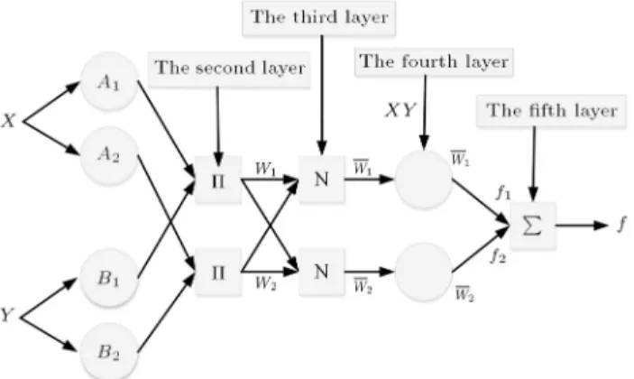
ANFIS is a fuzzy inference system performed in the structure of adaptive networks. The presented model can build an input-output mapping based on both human knowledge in the form of fuzzy rules and stipulated input-output data pairs. In the present study, it proposed a Sugeno-type fuzzy system in a ve-layer network (Figure 1) [28]. The node functions in the same layer are of the same function family as explained below:

- Layer 1: Every node i in this layer is a square node with a node function:

O1

i = Ai(x) ; (9)

where x is the input to node i, and Aiis the linguistic

Figure 1. Structure of ANFIS with two inputs and two rules.

label (such as \small" or \large") associated with this node function. In other words, O1

i is the

membership function of Aiand denes the degree to

which the given x fullls quantier Ai. Any

continu-ous and varicontinu-ous functions, such as generally applied bell-shaped, trapezoidal or triangular-shaped mem-bership functions, are ecient candidates for node functions in this layer.

- Layer 2: Every node in this layer is a circle node termed that multiples the incoming signals and sends the product out. For example:

wi= Ai(x) Bj(y) ; i = 1; 2: (10)

Each node output describes the T-norm operators that combine the probable input membership grades in order to calculate the ring strength of a rule. - Layer 3: Every node in this layer is a circle node

termed N. The ith node computes the ratio of the ith rule's ring strength to the sum of all rules' ring strengths:

wi=_w wi

1+ w2; i = 1; 2: (11)

For accessibility, outputs of this layer will be labeled as normalized ring strengths (Figure 2).

- Layer 4: Every node i in this layer is a square node with a node function:

O4

i = wifi= wi(pix + qiy + ri) ; (12)

where wi is the output of Layer 3, and fpi; qi; rig

is the parameter set. Parameters in this layer will be applied as consequent parameters that are adaptable.

- Layer 5: The single node in this layer is a circle node (adaptive node) termedPthat calculates the total output as the summation of all incoming signals, i.e.:

O5

i = overall output =

X

i

wifi=

P

iwifi

P

iwi : (13)

It is not adaptable.

To have knowledge of ANFIS, a combination of two

methods of back-propagation (gradient descent) and least squares estimation is applied. First, parameters of the introduction section are assumed stable, and nal parameters are estimated by applying the least squares method. Then, nal parameters are assumed stable and error back-propagation is applied to correct the parameters of introduction. This procedure is repeated in each learning cycle [29].

Two methods are generally applied to create AN-FIS: Grid Partition (GP) and Subtractive Clustering (SC). ANFIS with GP algorithm applies a hybrid-learning algorithm to recognize parameters of the inference system. It uses a combination of the least square method and the back-propagation gradient de-scent method for training ANFIS membership function parameters.

Grid partition divides the data space into rect-angular sub-spaces applying axis-paralleled partition based on the pre-dened number of MFs and their categories in each dimension. The number of rules is based on the number of input variables and that of MF applied per variable, and this partition strategy re-quires a small number of membership function for each input. It faces problems when we have a moderately large number of inputs [30].

Clustering is a task of selecting a set of data into groups, named clusters, to nd structures and patterns in a dataset, and the radius of a cluster is the maximum distance between all the points and the centroid. There are two most important clustering methods: the hard clustering and the fuzzy clustering. The hard clustering is based on categorizing each point of the dataset just to one cluster. In fuzzy clustering, objects on the borderlines among several clusters are not forced to fully relate to one of them. The Subtractive Clustering method (SC) as a hard clustering was suggested [31].

Based on the SC method, per data point is a potential cluster center and computes the potential for each data point based on the density of surrounding data points. The capacity of potential for a data point is a function of its distance to all other data points. A data point with many other surrounding data points will have a high potential value. The data point with the highest potential is chosen as the rst cluster center, and the potential of data points near the rst cluster center is demolished. Therefore, data points with the highest remaining potential as the next cluster center and the potential of data points near the new cluster center are demolished.

It is remarkable that the important radius of cluster is vital for deciding the number of clusters, and data points outside this radius have little eect on the potential decision. Moreover, a smaller radius results in many smaller clusters in the data space, leading to more rules [31].

In this study, GP, SC, and another technique,

named Fuzzy C-Means (FCM), are applied to generate the ANFIS model. FCM is a strong unsupervised algorithm. FCM clustering was rst suggested by Dunn [32]. Bezdek (1981) extended it. FCM is an al-gorithm where per data point has a membership degree between 0 and 1 to each fuzzy subset. In other words, each data in FCM can be related to all groups with various membership grades. The algorithm generates an optimal partition c by minimizing the weighted within the group sum of squared error function Jm[32]:

Jm= N X i=1 c X j=1 um

jid2(xi; vj) ; (14)

where X = fx1; x2; :::; xNg 2 Rm is the dataset in

the m-dimensional vector space, N is the number of data items, c is the number of clusters within 2 < c < N, uji is the degree of membership of xi in the jth

cluster, m is the weighting proponent on each fuzzy membership, vjis the prototype of the center of cluster

j, and d2_(x

i; vj) is distance measure between object xi

and cluster center vj.

To generate an ANFIS with FCM, data are clustered by FCM algorithm and, then, ANFIS method is used for clustering data.

3. Case study and analytical modeling

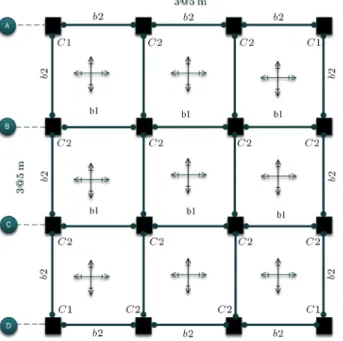
To evaluate eects of various sources of uncertainties and their interaction on the collapse fragility curves, a 3-storey intermediate moment steel building is designed for a specied site (Tehran), located in a high seismic zone. The seismic design of the case study structure is performed based on UBC-97 provisions [33]. This building is assumed to be constructed on soil type B (the average velocity of shear waves in the top 30 m of soil would be 360-750 m/s) and located in seismic zone 4. The buildings are square in plan and consist of three bays of 5.0 m in each direction with the story heights of 3.2 m, as shown in Figures 3 and 4.

A rigid diaphragm can be assumed according to the oor building systems existing in common steel con-crete composite oor structural systems. The values of response modication factors (i.e., R) are utilized by UBC-97 (considering R = 8:5 for special moment-resisting frame) [33]. Gravity loads are supposed to be similar to common residential buildings in Iran. Table 1 gives cross-sections for all members. The fundamental period of the frame is 1.075 s.

OpenSees nite-element program is employed for modeling and analysis of the structures. All frame members are modeled with the two-dimensional pris-matic beam element consisting of semi-rigid rotational springs at the ends and an elastic beam element in the middle (see Figure 5). The analytical model

Figure 3. Sample frame of the case study building.

Figure 4. The plane of sample building.

developed by Ibarra et al., referred to as Ibarra-Medina-Krawinkler (IMK) model, is applied in this study [35]. It has been shown that fp; pc; g

have more eects than other modeling parameters on collapse performance of structures [35]. Nonlinear behavior of frame members is simulated. The IMK

Figure 5. Modied beam element consisting of an elastic beam element with springs at both ends.

model creates strength bounds based on a monotonic curve, as shown in Figure 6.

Denitions of modeling parameters, shown in Figure 6, are as follows:

c Cap rotation;

My Eective yield moment;

Table 1. Design sections for the case study structure.

Story C1 C2 B1 B2

1 180 180 1:6 200 200 1:6 IPE 300 IPE 330 2 180 180 1:6 200 200 1:6 IPE 300 IPE 330 3 180 180 1:6 200 200 1:6 IPE 300 IPE 330

Figure 6. Back-bone curve of moment rotation model based on modied Ibarra-Krawinkler model [27].

u Ultimate rotation capacity;

P Plastic rotation capacity;

pc Post-Capping rotation capacity.

The hysteretic behavior of the connection is de-ned based on deterioration rules, which are dede-ned according to hysteretic energy dissipated in each load-deformation cycle.

The deterioration of basic strength, post capping strength, unloading stiness, and reloading stiness could be considered in this model. The energy dissipa-tion capacity of the component, by which deterioradissipa-tion rules are formulated, is described as follows [35]:

Et= My: (15)

In Eq. (15), is the rate of cyclic deterioration and is estimated according to calibration of experimental results. It has been represented that p, pc, and

have greater inuence than other modeling parameters on collapse performance of structures. Lognormal probability distribution function is employed to show uncertainties due to p, pc, and . The parameters

of these probability distributions, based on laboratory tests, are presented in Table 2.

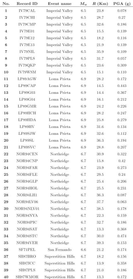
The inelastic beam-column joint behavior of the steel frame is simulated by nonlinear panel zone of Krawinkler model, shown in Figure 7. This model holds the full dimension of the panel zone with rigid links and controls the deformation of the panel zone using two bilinear springs that simulate a tri-linear behavior [36]. A set of 40 strong ground motions represented by Medina [37], named as LMSR records, is chosen to consider record-to-record variability in estimating col-lapse capacity of the structure. IM-based formulation is used to derive collapse fragility curves from performing IDA of the sample structure. These records include normal strong ground motions recorded in California region and do not involve pulse-type near-eld features, as introduced in Table 3. The hunt & ll tracing algorithm is used to scale records in IDA method to achieve good performance [16].

Fragility curves are developed by ANFIS based on the fuzzy C-means algorithm. To achieve input data and train ANFIS, ve realizations for each modeling random variable (p, pc, and ) are considered. It

is to be noted that they are related to mean, mean minus and plus one standard deviation, and mean minus and plus two standard deviations (mean, mean 1 standard deviation, mean 2:0 standard deviation, and totally 125 simulations). The tree diagram of realizations for input variables is shown in Figure 8. Each branch of the tree shows a value for one of input variables. For each realization of input variables, IDA is performed and collapse fragility curves are derived based on Eq. (3). The selected parameters for Intensity Measure (IM) and Damage Measure (DM) should appropriately indicate the im-pact of an earthquake and behavior of a construction, respectively. Maximum inter-story drift ratio among the common parameters is chosen to estimate DM. For IM parameter, spectral acceleration Sa(T1; 5%)

in fundamental elastic natural period among other intensity measures is selected. Both advantages of eciency and suciency are considered for Saintensity

measure while are used versus maximum inter-storey drift ratio [16].

Table 2. Mean and dispersion and correlation calibration of modeling parameters. Median p (rad) p

(rad)

Median pc

(rad)

pc

(rad) Median p;pc p; pc;

Table 3. Strong ground motion used for dynamic analysis. No. Record ID Event name Mw R (Km) PGA (g)

1 IV79CAL Imperial Valley 6.5 23.8 0.078

2 IV79CHI Imperial Valley 6.5 28.7 0.27

3 IV79CMP Imperial Valley 6.5 32.6 0.186 4 IV79E01 Imperial Valley 6.5 15.5 0.139 5 IV79E12 Imperial Valley 6.5 18.2 0.116 6 IV79E13 Imperial Valley 6.5 21.9 0.139 7 IV79NIL Imperial Valley 6.5 35.9 0.109 8 IV79PLS Imperial Valley 6.5 31.7 0.057 9 IV79QKP Imperial Valley 6.5 23.6 0.309 10 IV79WSM Imperial Valley 6.5 15.1 0.110

11 LP89AGW Loma Prieta 6.9 28.2 0.172

12 LP89CAP Loma Prieta 6.9 14.5 0.443

13 LP89G03 Loma Prieta 6.9 14.4 0.367

14 LP89G04 Loma Prieta 6.9 16.1 0.212

15 LP89GMR Loma Prieta 6.9 24.2 0.226

16 LP89HCH Loma Prieta 6.9 28.2 0.247

17 LP89HDA Loma Prieta 6.9 25.8 0.279

18 LP89HV Loma Prieta 6.9 31.6 0.134

19 LP89SJW Loma Prieta 6.9 32.6 0.112

20 LP89SL Loma Prieta 6.9 36.3 0.194

21 LP89SVC Loma Prieta 6.9 28.8 0.207

22 NOR94CEN Northridge 6.7 30.9 0.322

23 NOR94CNP Northridge 6.7 15.8 0.42

24 NOR94FAR Northridge 6.7 23.9 0.273

25 NOR94FLE Northridge 6.7 29.5 0.24

26 NOR94GLP Northridge 6.7 25.4 0.206

27 NOR94HOL Northridge 6.7 25.5 0.231

28 NOR94LH1 Northridge 6.7 36.3 0.087

29 NOR94LV06 Northridge 6.7 37.7 0.063

30 NOR94NLV01 Northridge 6.7 38.5 0.178

31 NOR94NYA Northridge 6.7 22.3 0.159

32 NOR94PIC Northridge 6.7 32.7 0.186

33 NOR94SAT Northridge 6.7 13.3 0.368

34 NOR94STC Northridge 6.7 30.0 0.474

35 NOR94VER Northridge 6.7 39.3 0.153

36 SF71PEL San Fernando 6.6 21.2 0.174

37 SH87BRO Superstition Hills 6.7 18.2 0.156 38 SH87ICC Superstition Hills 6.7 13.9 0.358 39 SH87PLS Superstition Hills 6.7 21.0 0.186 40 SH87WMOR Superstition Hills 6.7 13.3 0.172

Figure 7. Panel zone modeling [28].

Figure 8. Tree diagram for pre-assumed values of modelling parameters.

A total of number of 40 125 IDA curves are de-veloped to train and test the proposed ANFIS network in which 125 various of these p, pc, and parameters

are input data for ANFIS system. Objective data in ANFIS method are mean and standard deviation of

collapse fragility curves, which are similar to output functions in FOSM method.

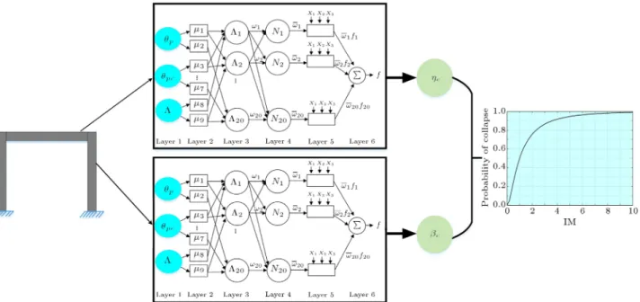
Figures 9 and 10 present a sample of IDA curves and fragility curves for 10 cases, and Figure 11 shows the architecture of represented neural networks to

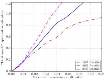
Figure 9. Samples for fractiles of IDA curve for p= 0:025, pc= 0:16, and = 1:0.

Figure 10. Samples of collapse fragility curves for 125 cases.

predict mean and standard deviation values of collapse fragility curves. As shown in this gure, after analyzing each scenario, including epistemic uncertainty, AN-FIS predicts mean and standard deviation of collapse fragility curves. There are 125 available data for

ANFIS, while 88 cases are applied for training and 37 remaining data for testing the model.

The performance of model conguration is esti-mated based on coecient (R) and Mean-Square Error (MSE) of the linear regression between the predicted values from the neural network model and the desired outputs as follows:

RMSE = ni

P_ni

i=1(yi ^yi)2

(ni 1)Pn_i=1i (yi)2; (16)

R2_{= 1}

"P_ni

i=1(yi ^yi)2

P_ni

i=1(^yi)2

#

; (17)

where y and ^y are actual and predicted values, respec-tively, and niis the number of testing samples. Smaller

RMSE and larger R2_{are generally indicative of better}

performance. To nd the best results based on GP, SC, and FCM methods, datasets are applied randomly and many models are established. It is discovered that the FCM model is much faster than the other two methods, and the algorithm of GP is a more time-consuming process than others are. Moreover, the results of the best models obtained from SC method are lower than those of both GP and SC methods. In the SC method, radius of the cluster should be dened before modeling. The smaller radius will create a greater number of unknown parameters. In Table 4, the best results obtained by the SC algorithm for the test phase are presented. According to this table, the best model has 0.89 and 0.029 for R and RMSE of the mean value of fragility curve, respectively. It is found that the GP algorithm has less error; however, more rules are needed to solve the problem. It is observed that to evaluate standard deviation, FCM algorithm has higher eciency than other two methods do. To create ANFIS with FCM algorithm, the number of clusters is predened for the model. Therefore, to get the proper state, many models with various clusters are established. The best model in the test and the train properties for the mean and the standard deviation are presented in Table 5.

Table 4. The results of the best models obtained from ANFIS by SC algorithm.

Number of clusters Number of rules R RMSE

The standard deviation of fragility curve 0.64 14 0.98 0.12

The mean value of fragility curve 0.62 9 0.89 0.029

Table 5. The results of the best models obtained from ANFIS by FCM algorithm. Number of

clusters

Partition matrix exponent

Maximum number of iterations

Initial step size

The standard deviation of fragility curve 14 1.41 200 0.01

Figure 11. The architecture presentation of ANFIS to predict fragility curve.

Figure 12. Comparison of the calculated mean of fragility curve based on IDA and ANFIS.

The performance of ANFIS for evaluating the mean values of test data for developing fragility curve is shown in Figure 12. The relevant value for the standard deviation is shown in Figure 13, where ANFIS output values are plotted versus the results achieved by performing full IDA.

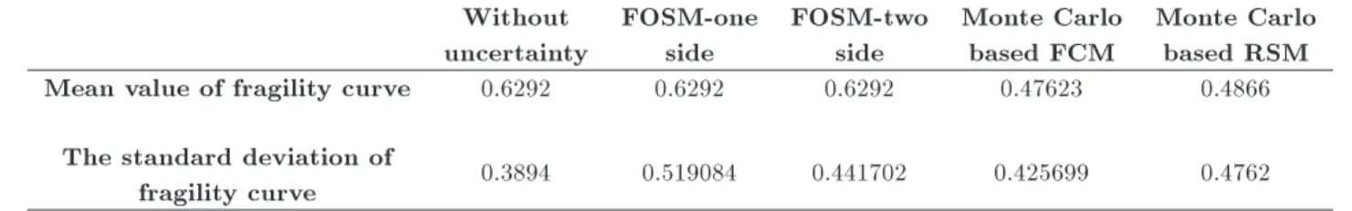
Two dierent training sets of the mean and the standard deviation have been tested, nding that both performed equally well; hence, ANFIS with FCM is chosen, since it requires lower computational time and better performance for preparing the training and testing set. To predict the means and standard deviations of collapse fragility curves, ANFIS based on fuzzy C-means algorithm simulation is applied. These models are calibrated from 10000 realizations of input random variables located inside interval [-2s, +2s]; then, collapse fragility curve is derived through tting a log-normal probability distribution. It is observed in Table 6 that the mean and the standard deviation of fragility curve in ANFIS method with FCM are 0.47623 and 0.4256, respectively. As a result, through a comparison while disregarding modeling uncertainties, the mean is reduced by 25% and the standard deviation is increased by 9.3%. The comparison between FOSM approximation, including modeling uncertainties, in developing fragility curves and resulted fragility curve, excluding modeling uncertainties, is noteworthy. The mean value does not change using FOSM approxima-tion. As presented in Table 6, mean and standard deviation of collapse fragility curve of the sample structure with neglecting modeling uncertainties are 0.6292 and 0.3894, respectively. Application of FOSM method to involve modeling uncertainty keeps mean value unchanged, and standard deviation changes to 0.5190 and 0.4417 for one-side and two-side formula-tions represented by Eqs. (7) and (9), respectively.

Results of quadratic response surface method and the proposed method are compared in terms of collapse fragility curves. To obtain input data to

evaluate response surface, ve realizations for each of modeling random variables (p; pc; ) are considered,

corresponding to mean, mean minus and plus one standard deviation, and mean minus and plus two standard deviations (totally, 125 simulations). For each realization of input variables, IDA is implemented and collapse-capacity spectral acceleration is derived for each record.

Response functions, applied to estimate mean and standard deviation of collapse fragility curves, are shown in Eqs. (18) and (19). The constant coecients of these equations are evaluated through implementing nonlinear regression analysis. Estimated coecients are listed in Table 7.

Implementing response surface functions in con-junction with Monte Carlo simulation derived the mean and standard deviation of fragility curve of 0.4866 and 0.4762, respectively (depicted in Table 6).

c= C0+ C1p+ C2pc+ C3 + C4ppc+ C5ppc

+C6pc + C72p+ C82pc+ C92; (18)

c= C00+ C01p+ C20pc+ C30 + C40ppc

+C50ppc+ C60pc + C70p2+ C80pc2 + C902:

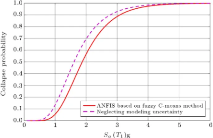
(19) Figures 14 and 15 show the resultant collapse fragility curves using ANFIS based on fuzzy C-means algorithm simulation, in addition to collapse fragility curve, irrespective of eects of modeling uncertainties (while modeling parameters are set as their mean values). 4. Conclusion

This paper introduced ANFIS and FCM train-ing/validation algorithm as an ecient and eective

Table 6. Results of FOSM, ANFIS, and RSM on parameters of collapse fragility curves. Without

uncertainty

FOSM-one side

FOSM-two side

Monte Carlo based FCM

Monte Carlo based RSM Mean value of fragility curve 0.6292 0.6292 0.6292 0.47623 0.4866

The standard deviation of

fragility curve 0.3894 0.519084 0.441702 0.425699 0.4762

Table 7. The coecients of RSM functions for mean and standard deviation of fragility curves.

C0 C1 C2 C3 C4 C5 C6 C7 C8 C9

The mean of fragility curve -3.47 244.10 3.29 1.10 -45.32 -5.25 1.09 -4655.55 -6.48 -.38 C0

0 C10 C20 C30 C04 C50 C60 C70 C80 C90

The standard deviation

Figure 14. Collapse fragility curves and comparison of various methods.

Figure 15. Comparison of including and excluding epistemic uncertainties in collapse fragility curves.

method to predict the mean and standard deviation values of collapse fragility curves of a case study of the three-story SMRF building. The modied Ibarra-Medina-Krawinkler moment rotation model was con-sidered as modeling parameters for frame's members. The fragility curves were derived through implementa-tion of IDA on the structure, while limited realizaimplementa-tions of values for modeling parameters were presumed. To this end, three inputs (P, pc, and ) and two

output data values (mean and standard deviation) were considered. The system was trained by a dataset of 125 values obtained from 5000 IDA curves. Then, the dataset consisting of 10000 inputs was applied to predict a basis fragility curve with aleatory and epistemic uncertainties. As a result, involvement of modeling uncertainties reduced the mean and increased the standard deviation of the obtained fragility curves. To compare the results, collapse fragility curves of the sample frame were derived using other approaches, such as FOSM and RSM methods. Modeling pa-rameters involved in moment-rotation relationship of connections, entitled (p, pc, and ), were considered

as epistemic uncertain parameters. The eects of epistemic uncertainties on collapse fragility curves were

estimated by the aforementioned methods. Many

ANFIS models based on GP, SC, and FCM were expanded, and it was understood that the ANFIS-FCM predicted the fragility curve with higher accuracy than other methods might (GP, SC). GP is a more time-consuming process than other methods and needs more rules to solve the problem; in the SC method, the problem is radius value of the cluster, which should be dened before modeling. Hence, the smaller radius may create a greater number of unknown parameters. In this respect, FCM algorithm has better eciency than other two methods do. Therefore, FCM algorithm in comparison with Monte Carlo method is known as a precise methodology. Nevertheless, the proposed method presented here demonstrates a small predic-tion error and leads to comparable results with those obtained using the Monte Carlo method.

References

1. Whittaker, A., Hamburger, R., and Mahoney, M.

\Performance-based engineering of buildings and in-frastructure for extreme loadings", in Proceedings, AISC-SINY Symposium on Resisting Blast and Pro-gressive Collapse, American Institute of Steel Con-struction, New York (2003).

2. Khurana, A. \Report on earthquake of 8th October in some parts of northern India", EERI (Earthquake En-gineering Research Institute), Special Reports (2005).

3. Liel, A.B., Haselton, C.B., Deierlein, G.G., and Baker, J.W. \Incorporating modeling uncertainties in the assessment of seismic collapse risk of buildings", Struc-tural Safety, 31, pp. 197-211 (2009).

4. Ibarra L.F. and Krawinkler, H., Global Collapse of Frame Structures Under Seismic Excitations, Pacic Earthquake Engineering Research Center (2005).

5. Benjamin, J.R. and Cornell, C.A., Probability, Statis-tics, and Decision for Civil Engineers, Courier Corpo-ration (2014).

6. Zareian, F., Krawinkler, H., Ibarra, L., and Lignos, D. \Basic concepts and performance measures in predic-tion of collapse of buildings under earthquake ground motions", The Structural Design of Tall and Special Buildings, 19, pp. 167-181 (2010).

7. Khojastehfar, E., Beheshti-Aval, S.B., Zolfaghari, M.R., and Nasrollahzade, K. \Collapse fragility curve development using Monte Carlo simulation and arti-cial neural network", Proceedings of the Institution of Mechanical Engineers, Part O: Journal of Risk and Reliability, 228, pp. 301-312 (2014).

8. Beheshti-Aval, S.B., Khojastehfar, E., Noori, M., and Zolfaghar, M.R. \A comprehensive collapse fragility assessment of moment resisting steel frames consider-ing various sources of uncertainties", Canadian Jour-nal of Civil Engineering, 43(2), pp. 118-131 (2016).

9. Lagaros N.D. and Fragiadakis, M. \Fragility assess-ment of steel frames using neural networks", Earth-quake Spectra, 23, pp. 735-752 (2007).

10. Mitropoulou, C.C. and Papadrakakis, M. \Developing fragility curves based on neural network IDA pre-dictions", Engineering Structures, 33, pp. 3409-3421 (2011).

11. Cardaliaguet, P. and Euvrard, G. \Approximation of a function and its derivative with a neural network", Neural Networks, 5, pp. 207-220 (1992).

12. Li, X. \Simultaneous approximations of multivariate functions and their derivatives by neural networks with one hidden layer", Neurocomputing, 12, pp. 327-343 (1996).

13. Chapman, O. and Crossland, A. \Neural networks in probabilistic structural mechanics", in Probabilistic Structural Mechanics Handbook, pp. 317-330 (1995).

14. Atmaca, H., Cetisli, B., and Yavuz, H.S., The Compar-ison of Fuzzy Inference Systems and Neural Network Approaches with ANFIS Method for Fuel Consumption Data, Yavuz Osmangazi University, Electrical and Electronic Engineering Department (2001).

15. Farahani, M.K. and Mehralian, S. \Comparison be-tween articial neural network and neuro-fuzzy for gold price prediction", Fuzzy Systems (IFSC), 13th Iranian Conference on, At Qazvin, Iran (2013).

16. Vamvatsikos, D. and Cornell, C.A. \Incremental dy-namic analysis", Earthquake Engineering & Structural Dynamics, 31, pp. 491-514 (2002).

17. Zareian, F., Lignos, D.G. and Krawinkler, H. \Quan-tication of modeling uncertainties for collapse assess-ment of structural systems under seismic excitations", in Proceedings of the 2nd International Conference on Computational Methods in Structural Dynamics and Earthquake Engineering (COMPDYN 2009), pp. 22-24 (2009).

18. Beheshti-Aval, S.B., Verki, A.M., and Rastegaran, M. \Systematical approach to evaluate probability of steel MRF buildings based on engineering demand and intensity measure", Proc. of the Intl. Conf. on Ad-vances in Civil, Structural and Mechanical Engineering (2014).

19. Zareian F. and Krawinkler, H. \Assessment of prob-ability of collapse and design for collapse safety", Earthquake Engineering & Structural Dynamics, 36, pp. 1901-1914 (2007).

20. Celarec, D. and Dolsek, M. \The impact of modelling uncertainties on the seismic performance assessment of reinforced concrete frame buildings", Engineering Structures, 52, pp. 340-354 (2013).

21. Rubinstein, R.Y. and Kroese, D.P., Simulation and the Monte Carlo Method, 707, John Wiley & Sons (2011).

22. Esteva, L. and Ruiz, S.E. \Seismic failure rates of multistory frames", Journal of Structural Engineering, 115, pp. 268-284 (1989).

23. Baker, J.W. and Cornell, C.A. \A vector-valued ground motion intensity measure consisting of spectral acceleration and epsilon", Earthquake Engineering & Structural Dynamics, 34, pp. 1193-1217 (2005).

24. He, J.N. and Wang, Z. \Analysis on system reliability of steel framework structure and optimal design", Applied Mechanics and Materials, 105, pp. 902-906 (2011).

25. Seo, J. and Linzell, D.G. \Horizontally curved steel bridge seismic vulnerability assessment ", Engineering Structures, 34, pp. 21-32 (2012).

26. Liel, A.B., Haselton, C.B., Deierlein, G.G., and Baker, J.W. \Incorporating modelling uncertainties in the assessment of seismic collapse risk of buildings", Struc-tural Safety, 31(2), pp. 197-211 (2009).

27. Rajeev, P. and Tesfamariam, S. \Seismic fragilities for reinforced concrete buildings with consideration of irregularities", Structural Safety, 39, pp. 1-13 (2012).

28. Jang, J.S.R. \ANFIS: adaptive-network-based fuzzy inference system", Systems, Man and Cybernetics, IEEE Transactions on, 23, pp. 665-685 (1993).

29. Bezdek, J.C., Pattern Recognition with Fuzzy Objective Function Algorithms, Springer Science & Business Media (2013).

30. Jang, J.S.R., Sun, C.T., and Mizutani, E., Neuro-Fuzzy and Soft Computing; a Computational Approach to Learning and Machine Intelligence, Upper Saddle River, NJ: Prentice-Hall (1997).

31. Chiu, S.L. \Fuzzy model identication based on cluster estimation", Journal of Intelligent and Fuzzy Systems, 2, pp. 267-278 (1994).

32. Dunn, J.C. \A Fuzzy relative of the ISODATA pro-cess and its use in detecting compact well-separated clusters", Journal of Cybernetics, 3, pp. 32-57 (1973).

33. UBC \Uniform building code", in Int. Conf. Building Ocials (1997).

34. Ibarra, L.F., Medina, R.A., and Krawinkler, H. \Hys-teretic models that incorporate strength and stiness deterioration", Earthquake Engineering and Structural Dynamics, 34, pp. 1489-1512 (2005).

35. Ellingwood, B.R. and Kinali, K. \Quantifying and communicating uncertainty in seismic risk assess-ment", Structural Safety, 31, pp. 179-187 (2009).

36. Foutch, D.A. and Yun, S.Y. \Modeling of steel moment frames for seismic loads", Journal of Constructional Steel Research, 58, pp. 529-564 (2002).

37. Medina R.A. and Krawinkler, H., Seismic Demands for Nondeteriorating Frame Structures and Their De-pendence on Ground Motions, Pacic Earthquake En-gineering Research Center (2004).

Biographies

Fooad Karimi Ghaleh Jough was born in 1982. He obtained his BS degree in Civil Engineering from

Tabriz Azad University, Iran in 2006 and MSc degree in Structural Engineering from Sistan & Baluchestan University, Zahedan, Iran in 2008. He received his PhD in Earthquake Engineering from Eastern Mediter-ranean University, Famagusta, Turkey in 2016 and has been a faculty member at Sarab Branch of Islamic Azad University. His research interests include vulnerability assessment of existing buildings and use metaheuristic algorithms in seismic risk analysis.

Seyed Bahram Beheshti Aval is an Associate Professor at Civil Engineering Department at the K. N. Toosi University of Technology. He received his PhD

degree from the Sharif University of Technology (SUT) in 1999. He is responsible for teaching courses in design of reinforced concrete structures, energy methods in nite element analysis, seismic rehabilitation of exist-ing buildexist-ings, structural reliability, and probabilistic seismic analysis of structures. His research activi-ties include studies of seismic reliability analysis of structures, composite structures, and various problems in seismic design of structures. He has authored more than 50 published papers and two textbooks, entitled Energy Principles and Variational Methods in Finite-Element Analysis and Seismic Rehabilitation of Existing Buildings.