Bi-objective Economic statistical design of the joint Xbar and S charts
incorporating Taguchi loss function
2
Farzad Firouzi Jahantigh
,
1*
Abdul Sattar Safaeia
1Department of Industrial Engineering, Babol University of Technology, P.O. Box 47148 - 71167, Babol, Iran 2Department of Industrial Engineering, assistant professor, Department of Industrial Engineering, University of
Sistan and Baluchestan, Zahedan, Iran
Abstract
In this research, a bi-objective model for the economic-statistical design of the X-bar and S
control charts is proposed. The model minimizes out-of-control average time to signal as well as minimizing mean hourly loss-cost where it incorporates the Taguchi loss function. A statistical constraint is considered in the model to achieve the desired in-control time to signal. A non-dominated sorting genetic algorithm is developed to obtain the pareto optimal scheme of the control chart. Sensitivity analysis and comparison study with traditional economic models presents that the proposed bi-objective design of X-bar and S
control chart ensures a better approach to improve the quality system and increase the plans ease of use.
Keywords: Control Chart; Economic-Statistical Design; Average Time to Signal; Taguchi loss function; Bi-objective Optimization
1- Introduction and literature review
In general, loss is thought of additional manufacturing costs incurred up to the point that a product is shipped. After that, it is the customers, who bear the loss of quality costs. Initially, the manufacturer must pay the warranty costs. After the warranty period expires, the customer may pay for repair. But the manufacturer will eventually pay indirectly, the costs of not satisfying customers as a result of customers’ negative reactions. These are the costs which are highly difficult to capture and account for, such as customer inconvenience and dissatisfaction, and time spent by customers.
Taguchi proposes a different view of quality, one that relates it to cost and loss in monetary scale, not just to the manufacturer at the time of production but to the consumer and to society as a whole(Khattree and Rao, 2003). Taguchi defines quality as “the loss imparted by the product to the society from the time the product is shipped.” The objective of the quality loss function is the quantitative evaluation of loss caused by functional variation of a product.
In real-world situations, a certain function exists for each quality characteristic that uniquely defines the relationship between the economic loss and the deviation of the quality characteristic from its target value. Taguchi found the quadratic representation of the quality loss function to be an efficient and effective way to estimate the loss due to deviation of a quality characteristic from its target value.
*Corresponding author.
ISSN: 1735-8272, Copyright c 2016 JISE. All rights reserved
Journal of Industrial and Systems Engineering
Vol. 9, No. 1, pp 1-16
Winter (January) 2016
Use of a quadratic approximation for the quality loss function is consistent with this philosophy (Taguchi et al., 1989). More studies on the loss functions are presented by Shaibu and Cho (2006).
In the economic design of control charts, where the objective is to minimize implementation cost of the control chart, the loss function has been explored in the previous studies (see, e.g., (Taguchi et al., 1989, Moskowitz et al., 1994, Chou et al., 2000, Ben-Daya and Duffuaa, 2003, Serel and Moskowitz, 2008); (Niaki et al., 2010b, Pandey et al., 2011)). Additionally, Costs due to nonconformities when the process is in-control and out-of-control is usually treated constants in the economic designs of charts. Nonetheless, incorporating the concept of the quality loss function into economic design models takes the advantages of both Taguchi concepts and statistical process control, which penalizes any deviation from the target, whether the system is in-control or out-of-control.
Moreover, when considering the cost associated with the implementation of the chart on one hand, and improved detection power of the chart on the other hand, the quality performance will play an important role as well. Thus, several researchers studied the economic-statistical design of control charts (see, e.g.(McWilliams et al., 2001, Bakir and Altunkaynak, 2004, Chen and Yeh, 2009)).
In many cases, the quality performance is related to the immeasurable portion of the system quality costs; i.e. the earlier detection of assignable cause initiates better reflections from the customer’s view. Therefore, this paper aims to find schemes which increase the control chart speed in detecting process changes. A bi-objective economic-statistical design of theX −Scontrol chart considering a quadratic loss function is proposed that enable the practitioner to simultaneously monitor the variability in the process mean and variance. The optimal scheme of the joint control charts are obtained such that the mean hourly loss-cost is minimized as well as minimization of out-of-control average time to signal (denoted byATS1)
along with maintaining reasonable in-control average time to signal (ATS0).
The paper is organized as follows. In the next Section the bi-objective design of control chart is introduced. In Section 3, the bi-objective model for the economic-statistical design of X −Schart is developed. Section 4 describes the proposed solution algorithm to find the optimal solution of the model. In Section 5, an illustrative numerical example is given for demonstrating the applicability of the proposed methodology. Furthermore, some sensitivity analysis and a comparative study are performed to evaluate the performance of the procedure and to determine the effects of process shift parameters on the performance of the proposed model. Conclusions are given in the last Section.
2- Bi objective design of control charts
Some of cost parameters in economic models for instance, hourly cost due to nonconformities in products produced while the process is out-of-control and the cost of investigating a false alarm are difficult to accurately estimate in practice (Pignatiello and Tsai, 1988, Reynolds and Cho, 2006, Chen and Liao, 2004). These costs are difficult to estimate because they involve an immeasurable diminishment in customer good will and operator’s confidence on the control chart. In addition, some processes simply cannot be sampled at unusual time intervals (Yeong et al., 2011).
To overcome this barrier, multi criteria optimization is studied in economic design of control chart. (Celano and Fichera, 1999) developed a X chart considering the optimization of the costs and the
statistical proprieties simultaneously, whereas in the multi-objective configuration, the fitness is the expected loss per hours multiplied by a coefficient function of the weighed sum of Type-I error probability and power of the chart. Such an approach is employed by Bakir and Altunkaynak (2004) to develop X −Rchart. Chen and Liao (2004) formulated an optimal design of X control chart into a
multiple criteria decision-making problem. Their solution procedure is based on data envelopment analysis. Asadzadeh and Khoshalhan ( 2008)developed a procedure to derive a multi objective decision making model with multiple assignable causes.
However, none of the above mentioned procedures guarantee improvement in the variation detection speed of the chart and increase the process monitoring costs. Further, a chart designer desires to find a solution with minimum cost and a reasonable detection power of the chart in the economic-statistical design of control charts. Detection power of the chart could be declared by several metrics. Type-I error
probability, power of the chart, in-control and out-of-control average run length (ARL),ATS0 and ATS1 are
the most usual metrics for describing the statistical properties of a control chart.
Since the sampling interval is altering within the pareto solution of bi objective design of control chart, it would be more appropriate to use average time to signal, instead of ARL, to evaluate the performance of the chart. In particular, the Pareto solutions reported by Chen and Liao (2004) and Asadzadeh and Khoshalhan ( 2008) for X control chart scheme are shown in Table (1). Note from this table that the solution with sample size of n=26, sampling interval of h=0.6 hours and X control limit coefficient of LX =2.9, outcome of 92.1238 with ATS1= 0.61 hours and Type-II error probability of β =
0.014, when another solution from the pareto set results a higher cost of 93.6692 with n=30, h=0.6 hours and LX =3.8, whereas ATS1= 0.63 hours and β = 0.047 did not been improved. More recent studies with
multi objective approach to control chart design has been published (Faraz et al., 2014, Faraz and Saniga, 2013, Morabi et al., 2015, Amiri et al., 2013, Safaei et al., 2012b, Safaei et al., 2012a, Amiri et al., 2014).
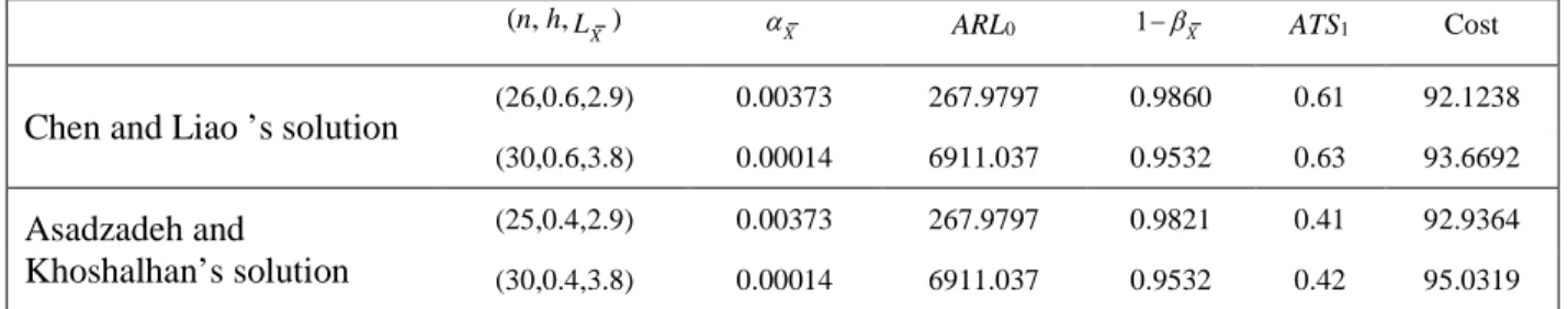
Table 1. solutions reported by Chen &Lioa and Asadzadeh &Khoshalhan’s procedure
(n, h,LX) αX ARL0 1−βX ATS1 Cost
Chen and Liao ’s solution
(26,0.6,2.9) 0.00373 267.9797 0.9860 0.61 92.1238
(30,0.6,3.8) 0.00014 6911.037 0.9532 0.63 93.6692
Asadzadeh and Khoshalhan’s solution
(25,0.4,2.9) 0.00373 267.9797 0.9821 0.41 92.9364
(30,0.4,3.8) 0.00014 6911.037 0.9532 0.42 95.0319
The ATS is defined as the average length of time and takes theX−Schart to produce a signal. When the process is in-control, the larger the value of ATS0 results the lower false alarm rate, whereas when the
process is out-of-control, the smaller the value of ATS0 result quicker detection of the assignable cause.
Minimization of the ATS1 results an earlier detection of out-of-control conditions. Moreover,
minimization of the ATS1 is cooperated as quality performance indices in the model to take another
consideration to the aspect of immeasurable costs. Indeed, to force the optimization model to outcome solutions that are acceptable from the economic viewpoint and the time needed to detect the out-of-control condition simultaneously, the optimal values of the out-of-control chart parameters are determined such that mean hourly loss-cost of the company and average time to signal in out-of-control state is minimized concurrently.
To leave behind the above-mentioned difficulties, a model that considers both measurable and immeasurable costs in a framework of bi objective economic-statistical design of jointX −Scontrol chart is proposed in this article. The average total loss, which is explained in the next section, will cover lost portions in the traditional economic models. The model provides a set of alternative solutions for quality manager to arrive at the requirement of long run quality of product along with minimal cost.
3- Bi objective joint
X- S chart
In this article, a measurable cost model is built upon the Lorenzen and Vance (1986)cost function. In addition, quality loss function approach is employed to estimate the immeasurable quality costs. A bi objective framework is utilized to determine the optimal scheme of economic statistical designed X −S
chart. FourX −Schart variables are assumed to be X control limitLX , S control limit LS , sample size n
and sampling interval h.
Consider a process in which the quality characteristic follow a normal distribution with mean µ0 and
standard deviation σ0 when the process is operating in-control; an X −Schart is applied to monitor the
process parameter mean and variance. The out-of-control process mean and the variance could be
µ1=µ0+δσ0 and be σ12=ρ2σ02 (ρ≥1), respectively. δ= (µ1 -µ0)/σ0 and ρ=σ1/σ0 are considered as shift
scenarios in the process mean and standard deviation. When an assignable cause that can change the mean
and variability of the process at the expected level is present, the joint probability of a Type I error can be computed as (McWilliams et al., 2001):
S S
X S X X
α
=α
+α
−α α
⋅ (1)X and S are statistically independent when sampling from a normal distribution. The joint power is computed as (McWilliams et al., 2001):
S S
X S X X
P =P +P −P ⋅P (2)
The false alarm rate (α) and the power of the X control chart (PX) are as follows (McWilliams et al.,
2001):
2 ( )
X LX
α = Φ − (3)
0.5 0.5
1 (( ) / ) (( ) / )
X X X
P = − Φ L −δn ρ + Φ −L −δn ρ (4)
Where Φ(.)is the cumulative probability distribution function (cdf) for a standard normal variable. The false alarm rate (α ) and the detection power of the S control chart (PS) are given by (McWilliams et al.,
2001):
2
1 (( 1) )
S G n LS
α = − − (5)
2 2 2
1 0
1 (( 1) /( / ))
S S
P = −G n− L σ σ (6)
Where Gn-1(.) is the cdf of the chi-squared probability distribution with (n−1)degrees of freedom.
The statistical measures considered in the model are as follows: The in-control average run length
0 1 / X S
ARL =
α
, the out-of-control average run lengthARL1= 1 /PX S, the in-control average time tosignalA TS0 =h A RL( 0), where h is the interval between successive samples, and the out-of-control average time to signalA TS1=h A RL( 1).
The expected quality cost per hours
E A
( )
, is computed as the fraction of the expected cost per cycle( )
E C
, to the expected cycle timeE T
( )
. Expected quality cycle time for a process is defined as the average time from control state until the assignable cause is identified and the process back to the in-control state. The in-in-control time for the process is assumed to be exponentially distributed with mean1 /
λ
.Equation (7) gives the expected cost per unit time (hours)(Lorenzen and Vance, 1986), E(A), associated with a control chart:0 1 1 1 1 2 2 1 2
1 1 1 2 2 3 0 3
1 1 2 1
( ) ( ) ( ) { / [ ] [( ) / ]
[1 / ] / } {1 / (1
E A E C E T C C A TS nE T T a a n h
A TS nE T T sa A RL a
A TS nE T T
λ
τ
γ
γ
λ
τ
γ
γ
λ
τ
γ
= ÷ = + − + + + + +
′
× + − + + + + +
÷ + − + + + + − )[sT0/A RL0]}
(7)
Where C0 is the cost per hours due to nonconformities in products produced while the process is
in-control; C1is the cost per hours due to nonconformities in products produced while the process is
out-of-control; E is the spent time to sample and chart one item; T0 is the expected search time when the signal is
a false alarm; T1 is the expected time to discover the assignable cause; T2 is the expected time to repair the
process; γ1 is 0 or 1 if production continues or ceases during searches respectively; γ2 is 0 or 1 if
production continues or ceases during repair respectively; s =e−λh/(1−e−λh)is the expected number of samples taken while in control; a1is the fixed cost per sample; a2 is the cost per unit sampled; a3is the
cost to locate and repair the assignable cause and
a
3′
is the cost per false alarm; and τ is the expected time between the occurrence of the assignable cause and the time of the last sample taken before the assignable cause which occurs between the jth and (j +1) th samples(Lorenzen and Vance, 1986), given in (8)(8)
Furthermore, in order to incorporate the intangible external costs based on the loss function, let T be the target value for the quality characteristic monitored and K the Taguchi loss coefficient. Also, let the
) 1 ( ) 1 ( 1 ) ( ) 1 ( ) 1 ( h h h j jh t h j jh t e e h dt e dt e jh t λ λ λ λ λ λ λ λ τ − − + − + − − + − = − =
∫
∫
4probability density function (pdf) of the quality characteristic X to be f(x). Then, the quality loss is zero only when the quality characteristic X equals the target T. The loss increases as the deviation from the target increases. If the loss function, L(X), is symmetric around the target, the loss coefficient K should be estimated such that the loss can be obtained as (Safaei et al., 2012a):
2
( ) ( )
L X =K x −T (9)
Here, the expected external costs of each product are shown by J0 and J1. To design control charts
based on a symmetric quadratic loss function, the expected cost per unit under quadratic loss function when the process operating in-control (J0) is calculated as (Safaei et al., 2012a):
] ) ( [ ) ( ) ( ) ( )
( 2 0 0 2 02 0 2
0 K x T f x dx K x T f x dx K T
J =
∫
− =∫
− + − = −+∞ ∞ − +∞ ∞ − µ σ µ µ (10)
Where f(x) is pdf of a normal variable with mean
µ
0and the standard deviationσ
0.The expected cost per unit under quadratic loss function when the process is out-of-control (J1) is as
(Safaei et al., 2012a):
2
1 1 1
2 2
1 0 0
2 2
1 0 0
2 2 2 2 2
0 0 0 0 0
( ) ( )
( ) ( ) ( ) ( )
= ( )
( ) 2 ( )
J K x T f x dx
K x f x dx K T f x dx
K T
K T T
µ µ
µ µ δσ
σ µ δσ
ρ σ µ δ σ δσ µ
+∞ −∞ +∞ +∞ −∞ −∞ = − + − = − + + − + + − = + − + − −
∫
∫
∫
(11)Note that the variability in process explicitly enters the cost function by means of the term C1 when a
loss function is used for computing the quality costs. If p units are produced per hours, C0 and C1 in cost
function, equation (7), can be computed as, C0=J0p and C1=J1p.Optimal values of the chart are determined
such that the new loss-cost function, say the Average Total Loss of the company (ATL), is minimized. One should be careful when employing economic control charts. Economic designs can yield solutions that are unwise in practice ((Woodall, 1986) and (Saniga, 1989)). Recalling Table (1), assume that during monitoring the process using X chart; the time to take sample and interpret the results is a constant proportional to the sample size (n) and an average time of 1 minute (0.0167 hours) needs to test and analyze a sample item (E = 0.0167 hours), one notes that these plans are awkward solutions. For instance solution vector with n = 30, h = 0.4 hours and L = 3.8 needs 0.5 hours (n * E = 30 * 0.0167 hours) for taking the samples and interpreting the results; while this is not consistent with the plan that recommends sampling every 0.4 hours. Such are the cases in several previous researches (see e.g. (Chen and Liao, 2004) and (Asadzadeh and Khoshalhan, 2008), (Serel, 2009) and (Faraz et al., 2011)).
Here the problem is solved by introducing a new constraint. On the other hand, this flexibility is one of the advantages of economic statistical design. A new constraint,nE≤h, ensures that optimal plans are meaningful and applicable in practice. This constraint decline schemes that the time of taking and charting samples goes beyond the sampling interval (h).
Additionally, the model should reduce too many false alarms that pure economic model can cause (Woodall, 1986). Saniga (1989) placed statistical constraints on an economic model to combine the benefits of both pure statistical and economic designs. However, one can see plans with too large ARL0
within existing literature; this may not be practical in some situations. For instance, solution reported by Chen and Liao (2004) and Asadzadeh and Khoshalhan (2008), presented in Table (1), suggest that ARL0 =
6911.037 which severely increases the monitoring costs.
To prevent this type of increasing in the process monitoring costs, the constrained optimization will be utilized which forces the model to generate solutions closer to the preferred ATS0. The constraint
ATS0 ≥ ATSL maintains a reasonable false alarm rate as well to minimize ATL and ATS1. Further, some
industrial applications and preferences require constraints on the model decision variables (n, h,LX and
LS).
The optimal values of the control parameters are determined such that the average total loss of the company and out-of-control ATS are minimized. Then, the bi objective economic-statistical model for joint X −S chart becomes as follows.
integer positive a is 0 and , ) , , , ( 0 1 n L L h h nE ATS ATS to Subject ATS Min h n L L ATL Min S X L S X > ≤ ≥ (12)
A solution algorithm is proposed to solve the bi objective optimization model given in (12) in the next Section.
4- The solution algorithm
In order to solve multi objective problems, two ideologically opposed sets of techniques can be chosen (Ehrgott and Gandibleux, 2003 and Augusto et al., 2006). The first set contains single objective optimization techniques that consist of building a function aggregating all of the objectives of the problem in a single function, which is supposed to represent designer’s preferences information. Such techniques provide a unique solution that is strongly linked with the aggregation function. Consequently, single-objective techniques can be considered “a priori” methodologies. The second set contains multi single-objective optimization techniques that provide a set of alternative solutions. They are based on an “a posteriori” articulation of preference information in order to make a choice within a set of optimum solutions.
Elitist non-dominated sorting genetic algorithm (NSGA-II), the multi objective evolutionary algorithms (MOEA) developed by (Deb, 2001), is one of the multi-objective optimization techniques that effectively provides a set of alternative solutions, the pareto optimal solutions. Optimization through pareto dominance compares each objective only with itself, removing the need for standardization of objectives, as well as the arbitrary nature that it adds to the optimization process (Carlyle et al., 2003). Since two of the model variables,LX and LS, are indirectly used in the model and is solely used for the
calculation of ARLs and ATSs, a genetic algorithm can be applied to solve the economic-statistical model (Niaki et al., 2010a). In this paper, pareto optimization is utilized and an elitist non-dominated sorting genetic algorithm (NSGA-II) is developed to optimally determine the solution vector.
Here the decision variables of the model areL , LX S, n and h. Consequently, a chromosome is
composed of four genes and each gene represents a decision variable. In the solution algorithm, population size of 150 is first randomly initialized, which then allows the parameters ATL, ATS1 to be
computed and the feasibility of constraint to be checked for each scheme. Populations that satisfy practical and statistical constraints evaluated based on ATL and ATS1; otherwise, that scheme penalized to
be eliminated within the elite population for next generation.
It is also very important to maintain the diversity of population for convergence to an optimal Pareto front. This is performed by controlling the elite members of the population as the algorithm progresses. The pareto fraction, limits the number of individuals on the pareto front. Moreover, crowding distance finds the relative closeness of a solution to other solutions on same rank; many individuals can have same rank where rank (1) is the best. After ranking and computing the crowding distance, new population of best individuals will be selected. Imported chromosomes from the previous steps will be inputs of the crossover operation; mutation step in each loop creates the mutated children using adaptive mutation.
Then objectives and constraints for this intermediate population will be evaluated. Here the pareto fraction of 50% and the low value of crossover fraction (say 10%) and mutation rate of 60% are applied;
these values were reached by trial and error using numerical examples to obtain better quality solutions. Finally, steps repeat until the termination criterion is reached; this criterion is the number of generations in this article. At the end of these steps, chromosomes, four chart variables (LX , LS, n, h),
with pareto optimality are reported as the alternative scheme for bi objective economic-statistical design of X −Scontrol chart. In the next section, the proposed scheme procedure is shown through an illustrative example.
5- Illustrative example
In this section numerical data that was originally given by Serel and Moskowitz (2008), with some modifications, is used to illustrate both the application of the developed bi objective economic statistical
X −Scontrol chart and the proposed algorithm. In this example, the cost and process parameters to solve the optimization model are: a1 = 5, a2 = 1, a3 = 250, a´3 = 500, E= 0.5 hours, T0 = 2 hours, T1 = 20 hours, T2
= 0 hours, γ1 = 1, γ2 = 0 and λ=0.01. On the average, the production rate of 200 units per hour is planned.
Assuming a quadratic loss function with K=0.1, σ02=1, µ0= T; If p=200 units are produced per hour, cost
per hour due to nonconformities produced while the process is in control (C0) or out of control (C1) are
computed as C0=200*J0 and C1=200*J1 and change in reference to shift in process mean and variance.
When the process mean and variance increases by δ=1.5 and ρ=1.5, C0 and C1 are 20 and 90 respectively.
In fact, cost penalty for producing in out of control states increases when the expected shifts are larger. The solution vector is (LX , LS, n, h) and the economic objective function that incorporates both
internal and external costs along with statistical objective is the comparative factor to evaluate different solutions. Furthermore, the designer prefers to take at least two products in each sampling scheme and at most 20 products can be evaluated in each sampling scheme. Moreover, the time between samples cannot be more than 20 hours, and to prevent more false alarms, the charts coefficients are bounded. Then, the following limits on the decision-variables: 2 ≤ n≤ 20, h≤ 20 and LX &LS≤ 4 are defined. The minimum
allowable ATS0 is 500. The optimal X −Schart decision variables that minimize both the ATL and ATS1
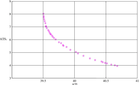
are given in Table (2). The pareto front for ATL and ATS1of the bi objective economic statistical design is
shown in Figure (2).
Table 2. Optimal design of X - S chart
X
L LS n h ATL ATS1 ATS0
2.92 2.24 5 5.12 39.51 8.02 1342.45
2.92 2.23 5 5.12 39.51 8.02 1358.62
2.92 2.24 5 5.00 39.51 7.83 1296.65
2.92 2.24 5 4.94 39.51 7.73 1280.43
2.92 2.26 5 4.83 39.52 7.59 1245.03
2.92 2.27 5 4.72 39.52 7.42 1205.60
2.90 2.35 5 4.63 39.54 7.27 1167.96
2.93 2.24 5 4.50 39.55 7.06 1164.78
2.91 2.28 5 4.48 39.55 7.03 1165.40
2.92 2.26 5 4.40 39.56 6.89 1112.08
2.93 2.29 5 4.26 39.58 6.74 1146.83
2.93 2.29 5 4.20 39.60 6.64 1130.02
2.92 2.27 5 4.15 39.61 6.53 1095.55
2.92 2.27 5 4.10 39.62 6.44 1082.25
2.94 2.26 5 4.06 39.63 6.42 1118.04
2.92 2.29 5 4.00 39.64 6.32 1046.44
2.93 2.27 5 3.95 39.66 6.23 1079.10
2.93 2.26 5 3.89 39.67 6.13 1049.51
2.95 2.24 5 3.80 39.70 6.02 1064.09
2.95 2.22 5 3.66 39.75 5.80 1033.97
2.98 2.24 5 3.56 39.79 5.72 955.02
2.94 2.29 5 3.51 39.82 5.57 973.19
2.92 2.28 5 3.50 39.83 5.52 915.11
2.92 2.38 5 3.41 39.87 5.42 934.85
2.93 2.23 5 3.30 39.94 5.20 832.94
2.90 2.45 5 3.19 40.02 5.04 827.25
2.92 2.31 5 3.11 40.06 4.92 832.66
2.95 2.23 5 3.00 40.14 4.74 789.08
2.93 2.23 5 2.90 40.25 4.54 719.28
2.93 2.23 5 2.80 40.33 4.41 706.77
2.95 2.34 5 2.68 40.43 4.28 804.67
2.93 2.32 5 2.68 40.45 4.24 754.98
2.95 2.26 5 2.64 40.49 4.19 765.27
2.91 2.26 5 2.64 40.52 4.14 696.50
2.96 2.19 5 2.53 40.64 4.00 694.72
2.91 2.26 5 2.51 40.68 3.94 663.50
Figure 2. Pareto front for ATL and ATS1
According to the presented Pareto set for theX−Schart in Table (2), the optimal scheme from the economic view point is where theX and S control limits coefficient areLX =2.92 and LS =2.24, and the
sample with size n=5 is obtained at time intervals of h=5.12 hours, while the achieved value of minimum
ATL is 39.51. For this solution, the statistical metrics are ATS1 =8.02 hours, ATS0 =1342.45 hours.
Due to the fact that the company concerns itself with long run quality of product more than looking for minimum cost; interestingly, one can see that at the same ATL= 39.51, the new scheme with the modification on the sampling interval, (2.92, 2.24, 5, 5.00), improves the speed of the X−S chart in detecting a process changes in ATS1 from 8.02 to 7.83 hours, where other statistical metrics are not quite
different. This solution will result earlier detection of the assignable cause where it receives a higher product quality. Moreover, a slight movement (0.01) from the minimum ATL to ATL= 39.52, the solution (2.92, 2.26, 5, 4.83) results more improvement in ATS1 = 7.59 hours.
On the other hand, calculating the pareto-optimal solution set may increase the plans ease of use. Chart designer may accept a solution with sampling frequency of h = 4.00 hours or h = 5.00 hours because of its administrative convenience. The scheme (2.92, 2.29, 5, 4.00) not only improves ATS1from
8.02 hours to 6.32 hours (approximately 21.25% improvement), but it also does not increase ATL
severely, here ATL is 39.64 (ATL increases 0.33%). It is important to note from the pareto set in Table (2) that theX and S control limit coefficients are varying along with the sampling interval whereas the sample size of n=5 did not changed.
Based upon alternative solutions presented in the pareto front, the company could prevent departure either way from the nominal value in production process with earlier detection of assignable cause and improve the quality of outgoing products that enhances customer’s goodwill. If statistical performance of the chart is an issue as well as the cost factors, the pareto solutions for ATL and ATS1 worth taking into
account. These results demonstrate that calculating the pareto optimal solution set is not only an effective way to perform optimum design, but it also is a practical way to obtain information to support quality control practitioners’ decisions.
ATL ATS1
39.5 40 40.5 41
3 4 5 6 7 8 9
6- Sensitivity analysis and comparisons
This Section first analyzes the sensitivity of the chart performance and Pareto solutions to variations in process shift parameters. Then, comparisons with economic statistical design of EWMA chart reported in (Serel and Moskowitz, 2008) are performed. To further investigate the effects of different process shifts, the process mean shifts of the sizes
δ
∈{0.5, 1.0, 1.5, 2.5} and standard deviation shifts of the sizesρ
∈
{1.0, 1.5, 2.0} are considered. Table (3) sums up the optimal chart parameters at loss function coefficientK = 0.1 with corresponding minimum ATL and ATS1of bi-objective design of X−Schart.
Table (3) presents three successive solutions in pareto front to show instances from the pareto solutions of 12run experiment. As it is obvious from Table (3), larger shifts in process mean and variance may be detected earlier through the X−S control chart with higher ATL. In addition, the pareto front in Table (3) presents solutions with improvement in ATS1 and a small additional impact in ATL.
As it is visible from Table (3), change in the sizes of shift in process mean and variance has significant effects on ATS1 in opposite way, where it is proportional to the ATL as it increases slightly at
steady state with increasing shift sizes. In most cases, improvement in ATS1 will incur small increase in ATL when the process faces smaller shifts that are harder to reach for the larger shift sizes. One of the main reasons of this change is increase in cost per hour due to nonconformities (C1); this term comes up
from the Taguchi loss function (C1=J1p) explicitly forces larger cost penalty to ATL with increasing in the
sizes of shift in the process. It is notable that the control limit coefficients and the sampling interval are varying in the Pareto sets whereas the sample size is not changing in most cases.
Table 3. Sensitivity analysis of X−S control chart
Bi-objective economic-statistical design of X−Schart
subject to ATS0 ≥500
Joint EWMA
No. δ ρ LX LS n h ATL ATS1 ATS0 Өm Өv Lm Lv n h ATL
1 0.5 1.0 2.88 3.14 15 20.00 24.97 115.49 5000.18 0.35 0.35 3.25 2.15 6 12.20 24.89 2.88 3.01 16 19.93 24.98 105.10 4999.19
2.88 3.14 16 19.88 24.98 104.66 4970.22
2 1.5 3.23 1.58 13 9.08 32.75 19.90 2420.77 0.63 0.59 3.35 2.10 9 6.80 32.63 3.23 1.58 13 9.01 32.75 19.74 2384.67
3.23 1.58 13 8.97 32.75 19.64 2351.44
3 2.0 3.28 1.90 6 5.11 39.18 9.03 1642.41 0.50 0.72 3.35 2.10 8 6.49 39.47 3.28 1.90 6 5.00 39.19 8.84 1348.22
3.31 1.89 6 4.93 39.19 8.71 1270.62
4 1.0 1.0 2.88 3.49 13 16.14 28.67 21.06 4035.51 0.34 0.20 2.90 2.00 4 5.45 29.12 2.89 3.35 13 15.55 28.68 20.34 3975.45
2.88 3.86 13 14.99 28.68 19.56 3765.19
5 1.5 2.98 1.85 8 6.71 35.21 12.37 1696.27 0.50 0.20 3.00 1.90 5 4.20 35.37 2.98 1.85 8 6.58 35.21 12.13 1682.25
2.98 1.85 8 6.53 35.21 12.04 1739.48
6 2.0 3.15 2.04 5 4.51 41.98 7.67 1337.49 0.49 0.68 3.38 2.14 7 5.45 42.46 3.21 2.02 5 4.35 41.98 7.43 1451.77
3.21 2.02 5 4.31 41.99 7.37 1454.19
7 1.5 1.0 2.88 4.00 6 7.95 33.67 10.10 1992.21 0.50 0.15 3.00 1.90 4 4.45 34.10 2.90 3.95 6 7.86 33.68 10.07 2106.28
2.91 3.97 6 7.67 33.69 9.88 2147.25
8 1.5 2.92 2.24 5 5.12 39.51 8.02 1342.45 0.60 0.15 3.00 1.90 4 3.95 39.63 2.92 2.24 5 5.00 39.51 7.83 1296.65
2.92 2.24 5 4.94 39.51 7.73 1280.43
9 2.0 3.04 2.25 4 3.92 46.48 6.15 1048.88 0.55 0.35 3.00 1.90 4 3.20 46.94 3.12 2.26 4 3.69 46.50 5.90 1376.21
3.12 2.26 4 3.56 46.51 5.72 1341.12
10 2.0 1.0 2.90 4.00 4 5.67 40.21 6.57 1524.67 0.62 0.20 2.90 2.00 3 3.95 40.46 2.95 3.98 4 5.59 40.22 6.56 1771.86
3.00 2.85 4 5.18 40.23 6.15 1909.48
11 1.5 2.92 2.58 4 4.48 45.71 5.81 1204.02 0.67 0.20 2.90 2.00 3 3.70 45.75 2.96 2.58 4 4.23 45.71 5.54 1305.64
2.96 2.59 4 4.23 45.71 5.54 1305.36
12 2.0 3.01 2.63 3 3.25 52.71 4.91 859.23 0.76 0.20 2.90 2.00 3 3.20 52.98 3.05 2.69 3 3.15 52.72 4.83 996.39
3.10 2.68 3 2.99 52.73 4.64 1016.49
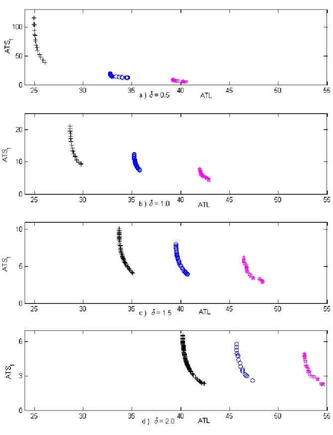
Figures (3) illustrate the pareto front for the 12 runs of the process parameter values. This figure plots the trends of ATL against ATS1 in the Pareto sets. Sections in Figure (3) are divided by process mean shift
of the sizes
δ
∈{0.5, 1.0, 1.5, 2.5}; i.e., section (a) presents the Pareto solutions for cases with small shift in process mean (δ =0.5). Also, three curves in each section of Figure (3) are representing the pareto front for X −Scontrol chart at fixed process mean shifts (δ) and standard deviation shifts of the sizesρ
∈
{1.0, 1.5, 2.0} respectively. In each section cases with ρ=1.0 shown in black colored plus signs, whereρ=1.5 exposed by blue colored circles and ρ=2.0 made known in purple asterisks.
Figure 3. Pareto front for Sensitivity Analysis of X - S chart
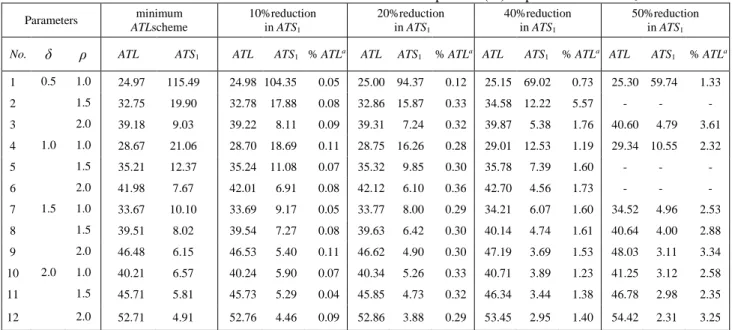
An extensive evaluation is given in Table (4). This Table analyzes the impact of improving ATS1 in ATL. From the pareto set, solutions with improvement close to 10%, 20% and 50% in ATS1 of the chart is
reported. For each solution ATL and ATS1 and increase in ATL is compared with the minimum reported ATL respectively. One can improve the chart performance with a slight increase in its ATL.
As shown in Table (4) and Figure (3), the smaller shifts in the mean and variance are resulted larger improvement in ATS1, and the better the efficiency of the Pareto sets. Among the numerical examples in
Table (4), in the first case when the process receives smallest shifts in the mean and variance, minimum hourly ATL is 24.97 and ATS1 is 115.49 hours. In this case, the solution from the pareto set which receive
10% improvement in ATS1 of the chart ensures that the cost of reducingATS1is less than 0.05% of the
minimum hourly ATL; here ATL changes from 24.97 to 24.98. Moreover, 20% earlier detection of the assignable cause yields a plan with simply0.12% more thanminimum hourly ATL in this shift levels.Accordingly, the Pareto set improved the performance of the standard X −Schart.
Table 4. Alternative solutions from Pareto sets with percent (%) improvement in ATS1
Parameters ATLminimum scheme 10%reduction in ATS
1
20%reduction in ATS1
40%reduction in ATS1
50%reduction in ATS1
No. δ ρ ATL ATS1 ATL ATS1 % ATLa ATL ATS1 % ATLa ATL ATS1 % ATLa ATL ATS1 % ATLa
1 0.5 1.0 24.97 115.49 24.98 104.35 0.05 25.00 94.37 0.12 25.15 69.02 0.73 25.30 59.74 1.33 2 1.5 32.75 19.90 32.78 17.88 0.08 32.86 15.87 0.33 34.58 12.22 5.57 - - - 3 2.0 39.18 9.03 39.22 8.11 0.09 39.31 7.24 0.32 39.87 5.38 1.76 40.60 4.79 3.61 4 1.0 1.0 28.67 21.06 28.70 18.69 0.11 28.75 16.26 0.28 29.01 12.53 1.19 29.34 10.55 2.32 5 1.5 35.21 12.37 35.24 11.08 0.07 35.32 9.85 0.30 35.78 7.39 1.60 - - - 6 2.0 41.98 7.67 42.01 6.91 0.08 42.12 6.10 0.36 42.70 4.56 1.73 - - - 7 1.5 1.0 33.67 10.10 33.69 9.17 0.05 33.77 8.00 0.29 34.21 6.07 1.60 34.52 4.96 2.53 8 1.5 39.51 8.02 39.54 7.27 0.08 39.63 6.42 0.30 40.14 4.74 1.61 40.64 4.00 2.88 9 2.0 46.48 6.15 46.53 5.40 0.11 46.62 4.90 0.30 47.19 3.69 1.53 48.03 3.11 3.34 10 2.0 1.0 40.21 6.57 40.24 5.90 0.07 40.34 5.26 0.33 40.71 3.89 1.23 41.25 3.12 2.58 11 1.5 45.71 5.81 45.73 5.29 0.04 45.85 4.73 0.32 46.34 3.44 1.38 46.78 2.98 2.35 12 2.0 52.71 4.91 52.76 4.46 0.09 52.86 3.88 0.29 53.45 2.95 1.40 54.42 2.31 3.25
Note from Table (4) that increase in the ATL is less than 0.11 % when one desire 10% improvement in ATS1 of the X−Schart. Furthermore, in the worst case the ATL increases almost 0.36% whereasATS1
improves 20%. On average, 50% improvements in time to release out-of-control signal can be obtained in less than 3.61% penalty cost.These findings mean that the bi-objective design of X −S chart is efficient.
Table (4) and Figure (3) verify the capability of the proposed approach in presenting pareto solutions that improve the time to signal out of control state where it has a slight impact in process monitoring costs. Besides, constraint ATS0 ≥ ATSL ensured reasonable average time to signal of in-control state for all
solutions in the pareto sets.
Furthermore, the pareto optimal solutions of the proposed bi objective economic statistical design of the X −Scontrol chart are compared with the traditional approach. Table (3) provides the comparison results between the minimum ATL1 within the pareto solutions of the proposed chart and the
economic-statistical design of joint EWMA chart design reported by Serel and Moskowitz (2008). In Table (3),Өm
and Өv are the smoothing constants associated with the EWMA chart for mean and variance, Lm and Lv are
the control limit parameter of the EWMA chart for mean and variance.
The results in Table (3) show that the proposed model has a better performance than the traditional approach in most cases except small change in both of process mean and variance; in sense of minimum
ATL.In other words, as opposed to a single-objective optimization problem that tries to find one single optimum solution with the intention of satisfying the imposed statistical constraints; the proposed bi-objective optimization model recommends a set of alternative optimum. Accordingly, this bi-bi-objective design of a control chart presents a better approach for practitioners to improve the quality of the process outputs.
7- Concluding remarks
Statistical properties in the economic statistical design of control charts is equally if not more important than the process monitoring costs. Therefore, this research explored the bi-objective economic-statistical design of X −S control charts for monitoring the process mean and variance. Through the proposed methodology, we determined the pareto optimal solution vector including the trade-off relationships between ATL and ATS1, which could not be determined by means of single objective approaches. In
addition, the relationship between the economic loss and the deviation of the quality characteristic from its target value is brought up in calculations by Taguchi quadratic loss function.
Generally, pareto frontiers illustrate that change in process shift size will affect both ATL and ATS1.
Moreover, when the shift in process variance is in its highest amount finding a solution with higher improvement in ATS1 will be more costly comparing to other variance shift scenarios. Both the optimal
sample size and sampling interval decrease along with increase in size of shifts in mean and/or variance. Analysis of the pareto frontiers proved that the proposed bi objective design of control chart reveals better solutions that substantially improve the performance of control chart power for faster detection of shifts in the process. Consequently, better quality may be achieved and the probability of the production in the out of control state will be decreased. Other results indicate the flexibility of bi-objective design of theX −S control chart. The resulting Pareto-optimal solution set provide information to help practitioners in selecting the most powerful plans in order to have the maximum protection over the shifts in process mean and/or variance.
In a practical sense, pareto solutions simply present alternative solutions that can overcome the barrier of awkward time intervals between samples that criticized in traditional economic design of control charts. The results reveal that the proposed methodology is worthy of recommendation and it is better for the process engineer to monitor the process by considering the Pareto solutions instead of designing the control chart by only one scheme.
Moreover, it is assumed that quality cycle follows a renewal reward process and the in control time for the process is exponentially distributed with mean 1/λ=100 hours, it is important to note that ATS0
greater than 500 hours is good enough and it is not essential to penalize the model by considering the
ATS0 as a new objective. Although, studding this with other data sets will promise another research.
Furthermore, researchers and academics may consider bi-objective design of adaptive control charts as the other potentially useful areas for future research.
References
Amiri, A., Bashiri, M., Maleki, M. R. & Moghaddam, A. S. 2014. Multi-objective Markov-based
economic-statistical design of EWMA control chart using NSGA-II and MOGA algorithms. International Journal of Multicriteria Decision Making, 4, 332-347.
Amiri, A., Mogouie, H. & Doroudyan, M. H. 2013. Multi-objective economic-statistical design of MEWMA control chart. International Journal of Productivity and Quality Management, 11, 131-149. Asadzadeh, S. & Khoshalhan, F. 2008. Multiple-objective design of an X̄ control chart with multiple assignable causes. International journal of advanced manufacturing technology, 43, 312-322.
Augusto, O. B., Rabeau, S., DE´Pince´, P. & Bennis, F. 2006. Multi-objective genetic algorithms: A way to improve the convergence rate. Engineering Applications of Artificial Intelligence 19, 501-510.
Bakir, M. A. & Altunkaynak 2004. The optimization with the genetic algorithm approach of the multi-objective, joint economical design of the x̄ and R control charts. Journal of Applied Statistics, 31, 753-772.
Ben-Daya, M. & Duffuaa, S. O. 2003. Integration of Taguchi’s loss function approach in the economic design of x¯chart. International Journal of Quality & Reliability Management, 20 607-619.
Carlyle, W. M., Fowler, J. W. & Gel, E. S., Kim, B. 2003. Quantitative comparison of approximate solution sets for bi-criteria optimization problems. Decision Sciences, 34, 63-82.
Celano, G. & Fichera, S. 1999. Multiobjective economic design of an X̄ control chart. Computers & industrial engineering, 37, 129-132.
Chen, F. L. & Yeh, C. H. 2009. Economic statistical design of non-uniform sampling scheme X bar control charts under non-normality and Gamma shock using genetic algorithm. Expert Systems with Applications, 36, 9488-9497.
Chen, Y. K. & Liao, H. C. 2004. Multi-criteria design of an X control chart. Computers & Industrial Engineering 46, 877-891.
Chou, C.-Y., Chen, C.-H. & Liu, H.-R. 2000. Economic-statistical design of X̄ charts for non-normal data by considering quality loss. Journal of Applied Statistics, 27, 939 - 951.
Deb, K. 2001. Multi-objective Optimization Using Evolutionary Algorithms, Chichester, UK, John Wiely.
Ehrgott, M. & Gandibleaux, X. 2003. Multiple criteria optimization: state of the art annotated bibliographic surveys, Kluwer Academic Publishers.
Faraz, A., Heuchenne, C. & Saniga, E. 2011. Optimal T2 Control Chart with a Double Sampling Scheme – An Alternative to the MEWMA Chart. Quality and Reliability Engineering International.
Faraz, A., Heuchenne, C., Saniga, E. & Costa, A. F. B. 2014. Double-objective economic statistical design of the VP T2 control chart: Wald's identity approach. Journal of Statistical Computation and Simulation, 84, 2123-2137.
Faraz, A. & Saniga, E. 2013. Multiobjective Genetic Algorithm Approach to the Economic Statistical Design of Control Charts with an Application to X¯bar and S2 Charts. Quality and Reliability Engineering International, 29, 407-415.
Khattree, R. & Rao, C. R. 2003. Statistics in Industry, Elsevier Publishing Company.
Lorenzen, T. J. & Vance, L. C. 1986. The Economic Design of Control Charts: A Unified Approach.
Technometrics, 28, 3-10.
Mcwilliams, T. P., Saniga, E. M. & Davis, D. J. 2001. Economic-statistical design of X̄ and R or X̄ and S charts. Journal of Quality Technology, 33, 234-241.
Morabi, Z. S., Owlia, M. S., Bashiri, M. & Doroudyan, M. H. 2015. Multi-objective design of control charts with fuzzy process parameters using the hybrid epsilon constraint PSO. Applied Soft Computing,
30, 390-399.
Moskowitz, H., Plante, R. & Chun, Y. H. 1994. Effect of quality loss functions on the economic design of x process control charts. European journal of operational research, 72, 333-349.
Niaki, S., Ershadi, M. & Malaki, M. 2010a. Economic and economic-statistical designs of MEWMA control charts—a hybrid Taguchi loss, Markov chain, and genetic algorithm approach. The International Journal of Advanced Manufacturing Technology, 48, 283-296.
Niaki, S. T., Ershadi, M. & Malaki, M. 2010b. Economic and economic-statistical designs of MEWMA control charts—a hybrid Taguchi loss, Markov chain, and genetic algorithm approach. The International Journal of Advanced Manufacturing Technology.
Pandey, D., Kulkarni, M. S. & Vrat, P. 2011. A methodology for joint optimization for maintenance planning, process quality and production scheduling. Computers & Industrial Engineering, 61, 1098-1106.
Pignatiello, J. J. & Tsai, A. 1988. Optimal Economic Design of X̄ Control Charts When Cost Model Parameters are Not Precisely Known. IIE Transactions, 20, 103-110.
Reynolds, M. R., JR. & Cho, G. Y. 2006. Multivariate Control Charts for Monitoring the Mean Vector and Covariance Matrix. Journal of Quality Technology, 38, 230-253.
Safaei, A., Kazemzadeh, R. & Niaki, S. 2012a. Multi-objective economic statistical design of X-bar control chart considering Taguchi loss function. The International Journal of Advanced Manufacturing Technology, 59, 1091-1101.
Safaei, A. S., Kazemzadeh, R. B. & Niaki, S. T. A. 2012b. Multiobjective Design of an S Control Chart for monitoring process variability. International Journal of Multicriteria Decision Making, 2, 408-424. Saniga, E. M. 1989. Economic Statistical Control-Chart Designs with an Application to X̄ and R Charts.
Technometrics, 31, 313-320.
Serel, D. A. 2009. Economic design of EWMA control charts based on loss function. Mathematical and Computer Modelling, 49, 745-759.
Serel, D. A. & Moskowitz, H. 2008. Joint economic design of EWMA control charts for mean and variance. European Journal of Operational Research, 184, 157-168.
Shaibu, A.-B. & Cho, B. 2006. Development of realistic quality loss functions for industrial applications.
Journal of Systems Science and Systems Engineering, 15, 385-398.
Taghchi, G., Elsayed, E. & Hsiang, T. 1989. Quality Engineering in Production Systems, New York, NY., McGraw-Hill.
Woodall, W. H. 1986. Weaknesses of the Economic Design of Control Charts. Technometrics, 28, 408-410.
Yeong, W. C., Khoo, M. B. C., Wu, Z. & Casatagliola, P. 2011. Economically Optimum Design of a Synthetic X¯ Chart. Quality and Reliability Engineering International, 28, 725-741.