Sharif University of Technology
Scientia IranicaTransactions E: Industrial Engineering http://scientiairanica.sharif.edu
An optimization model for emergency vehicle location
and relocation with consideration of unavailability time
S. Firooze
a, M. Raee
a;, and S.M. Zenouzzadeh
ba. Department of Industrial Engineering, Sharif University of Technology, Tehran, Iran.
b. Shool of Industrial and Systems Engineering, College of Engineering, University of Tehran, Tehran, Iran. Received 8 October 2016; received in revised form 1 June 2017; accepted 23 December 2017
KEYWORDS Ambulances; Emergency medical services;
Location; Relocation; Facility location.
Abstract.The main purpose of emergency medical services is to provide fast medical care, as well as to transport patients to the hospital in the shortest possible time. Healthcare managers try to improve healthcare systems through reducing the time it takes to respond to demands. In this paper, we seek to propose an optimization model in order to cover as much demand as possible in the shortest possible time using the available ambulance eet. To do so, considering the response and service time, amount of demand during the time periods, limitation in the number of available emergency vehicles and the capacity of ambulance stations, we have proposed a mixed integer linear programming optimization model, aiming to minimize the total response time. In this paper, we take into account eet relocation and unavailability time, the time interval in which the vehicle is on its way or doing a service at a demand point. Then, a sensitivity analysis is conducted on the model by manipulating the parameters to observe the eects on the outputs. In order to evaluate the model, several articial test problems were generated and solved. The results depict the capability of the proposed model in dealing with emergency cases.
© 2018 Sharif University of Technology. All rights reserved.
1. Introduction
Health infrastructure supports the health services. Due to the high cost of providing new facilities, there is always a tendency towards optimum use of the existing infrastructure. Health services can be categorized into three main categories: preventive, emergency, and centralized services. Preventive services include actions like vaccination, while centralized services consist of health centers. The main focus of this paper is on emergency services. Emergency services like ambulances provide vital care in order to save
*. Corresponding author. Tel.: +98 21 66165725; Fax: +98 21 66022702
E-mail addresses: rooze [email protected] (S. Firooze); [email protected] (M. Raee); [email protected] (S.M. Zenouzzadeh)
doi: 10.24200/sci.2017.20022
people's lives. The unpredictability of the time and place of emergency incidents is the main issue in this category. The emergency demand in these services is covered by the Emergency Vehicles (EV) located at xed points; therefore, the location of ambulances is important in service quality level. The main challenge in emergency services is to minimize the time it takes to respond to demands (i.e., the time between emergency call receipt and EV arrival to the demand point). Accordingly, special standards related to the response time to emergency demands have been established in dierent countries. For instance, in the U.S., this time is between 4 and 5 minutes for vital issues (e.g., heart attacks, severe accidents) [1]. Likewise, in BC, Canada, this standard is 9 minutes or less in urban areas [2].
Four steps are included in the process of respond-ing to an emergency demand in Emergency Medical Services (EMS): (1) incident detection and reporting, (2) call screening, (3) EV dispatch, and (4) actual
interventions at the scene. Incident detection is related to the moment that an emergency call is received. Next, the level of the incident is determined in order to nd the type as well as the number of ambulances needed to be dispatched. This step is one of the toughest challenges in EMS [3]. Hence, it is important to locate EVs properly at stations. Based on the level of the incident and other data, the appropriate ambulance is dispatched afterwards. The last step is to provide patients with initial interventions. Short response to demand time and returning to the emergency stations are essential in order for the EVs to be available and to cover the demand of upcoming periods.
In this paper, a new MIP model is presented to deal with the problem of emergency vehicles location and relocation. Unlike most of the previous works in the literature, eet relocation and unavailability time are considered. This results in higher utilization of the available eet and, therefore, higher service standards as well less needed eet to cover the demand. Using the presented model, a manager can get a holistic view of the system under his/her demand to evaluate changes and improvements.
In Section 2, the related works in the literate are reviewed briey. Then, in Section 3, the problem under study is described in detail. The proposed mathematical model is presented in Section 4. In order to illustrate the performance of the proposed model, a simple numerical example is presented and solved in Section 5. A sensitivity analysis is conducted on the proposed model, the results of which can be found in Section 6. In order to evaluate the capability of the model in dealing with dierent problems from dierent sizes, several test cases are solved in Section 7. Finally, we draw a conclusion in Section 8.
2. Literature review
Several studies have been conducted on EV location in recent decades. In this section, the previous related works are discussed. The common feature in most of the selected works is consideration of EV unavailability during service time. For further information about EV location, the interested reader can see the review papers available in the literature such as [3-9].
Two of the rst optimization models utilized frequently to formulate the EV location problem are Location Set Covering Models (LSCM) and Maximal Covering Location Problem (MCLP) proposed by Tore-gas et al. [10] and Church and Velle [11] for the rst time, respectively. In LSCMs, the aim is to minimize the number of ambulances needed to cover the demand. Both LSCMs and MCLPs do not consider many real-world aspects of the problem; the most important shortcoming of these models is that, once an ambulance is dispatched, some demand points are no
longer covered [3]. However, the main shortcoming of LSCMs is that they need too many emergency vehicles to deal with all the demands in the planning horizon. Later, some researchers have considered using MCLP models. These models maximize population coverage while taking limited eet constraint into account. Eaton et al. [12] applied MCLP in order to shake up EMS in Austin, Texas, which resulted in a $3.4 million construction cost cut down as well as a $1.2 million save per year through lowering operations costs. The base models were developed in dierent ways to address real-world conditions. A common way to develop classic models is to consider multiple vehicle types. One of the rst models in which multiple vehicle types are considered is Tandem Equipment Allocation Model (TEAM) proposed by Schilling et al. [13]. TEAM can be considered as a development of MCLP in which a new set of constraints is introduced in order to impose the hierarchy of vehicles. In the aforementioned mod-els, the coverage may be insucient during the busy time periods. To overcome this deciency, Hogan and ReVelle [14] proposed two dierent Backup Coverage Formulations called BACOP1 and BACOP2.
Some of the models, using a probabilistic ap-proach, attempt to maximize demand coverage. Ac-cording to Daskin [15], one of the leading proba-bilistic models proposed for EV location is Maximum Expected Covering Location Problem (MEXCLP). In this model, each EV is assumed unavailable by a predened probability, and EVs are independent of one another. Repede and Bernardo [16] extended MEXCLP by considering temporal changes in the daily demand, as well as spatial variation and multiple states of vehicle availability. The results show that their method was able to increase the number of calls covered in 10 minutes, from 84% to 95%. In addition, response time was reduced by 36%. In another study, Goldberg et al. [17] proposed a variant of MEXCLP in which the travel times were assumed to take values stochastically. The model attempted to maximize the number of calls covered within 8 minutes. The authors implemented the model on the data from Arizona, U.S., the result of which was a 1% increase in the expected number of calls covered within 8 minutes. Moreover, the worst covering ratio of a zone in time was increased from 24% to 53.1%. ReVelle and Hogan [18] propose two probabilistic methods, namely Maximum Availability Location Problems I & II (MALP I and MALP II), which are formulated as chance-constrained programming problems. An extension of LSCM was proposed by Ball and Lin [19], called Rel p, in which they utilized a linear constraint on the eet size needed to reach a predened reliability level.
Rajagopalan et al. [20] proposed a multi-period set covering location model for dynamic redeployment of ambulances. They sought to nd the minimum
num-ber of ambulances needed and their location in each time cluster in which the changes in the demand pat-terns were signicant. They also considered reaching a predened reliability level in demand coverage. Degel et al. [21] focused on the fact that, within a 24-hour cycle, the demand, travel time, speed of ambulances, and areas of coverage change and presented a new approach in order to maximize the coverage, which has been adjusted for variations due to daytime and site. A mixed-integer programming formulation was presented to formulate the location and relocation of EVs.
The focus in most of the recent works is on dynamic models and the unavailability of EVs and their relocation in order to cover the demand of upcoming time periods. Dynamic models are utilized to nd deployment/redeployment strategies when a number of ambulances are busy serving demand points. Dy-namic models can be seen to be in contrast to those strategies in which every ambulance is sent back to its 'home base' after visiting a demand node. In the majority of dynamic models, the aim is not to nd a good set of locations for the base points, but to nd the best strategies based on a given set of nodes. Dynamic models can aid managers make daily or even hourly plans to respond better to predictable demand uctuations by time and space [20,22]. One of these dynamic approaches, called Emergency Vehicle Rede-ployment Problem (EVRDP) [23], applies a dynamic ambulance management procedure, so as to control the unavailability of ambulances. Studies in this eld, mostly, applied real-time-based and multi-period-based approaches. In [24], a dynamic relocation system is developed for re companies in New York, U.S. Another dynamic model in the eld of EV relocation is Dynamic Double Standard Model (DDSM), proposed by Gendreau et al. [23], which utilizes the framework proposed by Gendreau et al. [25]. This model takes into account standard coverage and capacity constraints, as well as some dynamic features of the problem such as avoiding driving the same ambulance repeatedly, avoiding round trips, and avoiding long trips. Yang et al. [26] considered the dispatching and relocation of EVs in a single problem and used an online dispatch framework in order to improve the EV operations. Maxwell et al. [27] presented an approximated dynamic programming approach to decide where to redeploy the idle ambulances to maximize number of calls reached within a delay threshold. They formulated the program as a Markov decision process and proposed some approximations to the value function in order to deal with the high-dimensional and uncountable state space of the dynamic paradigm. Nogueira Jr et al. [28] proposed an optimization model to reduce emergency service response time via reallocation of ambulances to the bases. They also ran a simulation of their model to observe its performance in dynamic settings.
Schmid [29] solved the problem of location and reloca-tion of emergency vehicles using Approximate Dynamic Programming (ADP). They conducted some empirical tests on data derived from a real case in the city of Vienna. Their results showed a 13% improvement in the performance of the system under study. Knight et al. [30] proposed models focusing on the assumption of multiple patient classes. Their model aims to maximize the overall expected survival probability of multiple classes of patients. They also presented an approximation method to solve the stochastic version of their model. Belanger et al. [31] evaluated and analyzed dierent relocation strategies. The results of this study suggested that dynamic approaches, al-though more expensive, dominated static ones. A real-time approach to maximizing coverage with minimum possible total travel time was proposed by Enayati et al. [32]. They considered accumulated workload restrictions for personnel in a shift. The reported results showed a signicant improvement in average coverage. Yue et al. [33] proposed another simulation-based approach. The goal of their proposed approach was to position an entire eet of ambulances to base locations in order to maximize the service level/quality of the emergency medical services system. Alanis et al. [34] presented a two-dimensional Markov chain model of an emergency medical services system. This model relocated ambulances using a compliance table policy. For the purpose of validation, they utilized a detailed simulation model in dierent scenarios. Sudtachat et al. [35] considered a nested-compliance table, which restricts the number of relocations that can occur simultaneously. The nested-compliance table is modeled as an integer programming model aiming to maximize expected coverage. The authors determined an optimal nested-compliance using steady state probabilities of a Markov chain model. The relocations were considered as input parameters. One of the previous works that considered redeployment of EVs at a point other than their origin or base station is the paper presented by Jagtenberg et al. [22]. The authors claimed that although the problem was a dicult one in nature, it could be solved in real time with their proposed polynomial-time heuristic. Another paper that falls in this category is the work of van Barneveld et al. [36]. In their proposed heuristic redeployment method, the ambulances can idle at any desired node. Moreover, Majzoubi et al. [37] proposed integer linear, nonlinear programming model and an approximation method aiming to minimize the total travel costs, the penalty of not meeting response time window for patients, and the penalty of not covering census tracts. The main point of this work is that they have assumed that an ambulance can serve two demand points in one trip, i.e., an ambulance can pick up two patients in special occasions.
Multi-period redeployment problem (MDRDP) seeks to provide a redeployment plan based on the estimation of demand uctuations within the planning horizon [38]. Schmid and Doerner [39] developed the DSM approach so that it could be used in multi-period redeployment problems. In [40], a bi-objective model was proposed to minimize the number of ambulances used and also to minimize the number of redeployments within a shift. Naoum-Sawaya and Elhedhli [41] presented a two-stage stochastic optimization model for ambulance redeployment problem. To achieve a reasonable level of service, this model minimizes the number of relocations in the planning horizon. In their mode, the relocations are considered predetermined parameters; in other words, the reason for the unavail-ability of the ambulances is not strictly specied and it is only formulated as an input parameter of the model. The two-stage model presented by Lei et al. [38] takes into account the assumption of redeployment of EVs that are sent out for duty. In this model, travel times and demand are uncertain in each time period.
Reviewing the literature, we came to the conclu-sion that although many valuable studies have been conducted in this area and some of them, such as Jagtenberg et al. [22] and van Barneveld et al. [36], have considered the relocation of emergency vehicles, there are still some issues that are not addressed in the previous studies. In some studies, the expected fraction of later arrivals is minimized. This approach neglects to consider the unavailability time of emergency vehicles. In some other studies, the emergency vehicles are assumed to be relocated only at their based stations, which is not the case in many real-world situations. Therefore, in this paper, a mathematical optimization model is presented, in which both ambulance unavail-ability time and relocation are taken into account. We deal with relocation as a decision variable and a way to better utilize the available eet at hand.
3. Problem statement
In order to dispatch an ambulance, after call screening, it is necessary to consider two steps: (1) assigning ambulances to emergency stations and (2) relocating ambulances in emergency stations to cover the demand
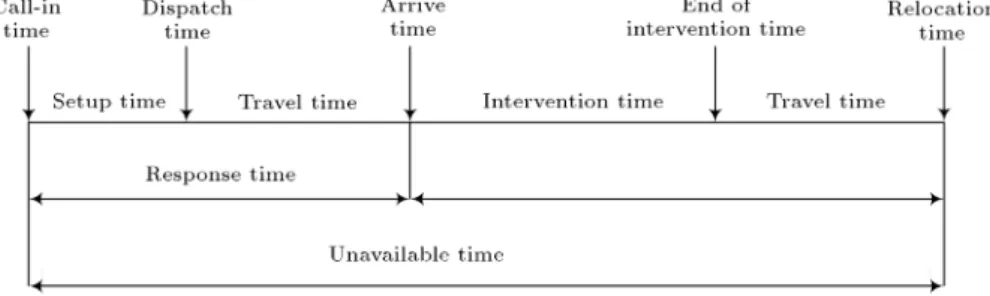
Figure 1. Emergency response process.
of upcoming periods. With respect to the status of EVs in each time period, the unavailable periods should be determined. Figure 1 shows that the collection of actions should be taken after an incident detection. In order to dispatch the EVs, it is required to determine the service time at the demand point, and the travel time to a new station for the purpose of relocation. The sum of these times is called the busy time (Figure 2). Hence, the ambulance is unavailable from the moement it is dispatched up to the time it is relocated at a new station. Accordingly, an approach is required to compute the number of available ambulances to cover the demand in a multi-period system.
Many of the existing models in the eld of location and relocation of EVs are single-period. However, in some recent studies, these issues are taken into consideration. Moreover, in most of the previous studies, as soon as an ambulance is sent out, it is eliminated from the eet, yielding poor performance of emergency system.
According to the literature, there are two types of ambulance in dierent countries: basic and advanced. Both types can respond to all demands; however, the advanced type is usually dispatched for cardiac arrest or similar situations when there is a need for a faster
service. Although the basic type can also be used to respond to this kind of demands, it takes longer to perform the service. In case of severe accident, more than one demand can perhaps be created in the same location. Considering this issue, the proposed model dispatches one ambulance for each demand, and the number of dispatched ambulance will be equal to the number of the demands.
Based on the aforementioned facts, in this paper, we aim to develop a model to provide maximum demand coverage in the least possible time for the planning horizon. In the proposed model, to provide high levels of conservatism, the length of each time period is assumed to be 1 minute (the reason is explained in Section 4.5 in detail). One of the features of the model is dividing EV busy time into dispatching, service, and return time. The objective functions attempt to minimize total dispatch and relocation time. It should be noted that, due to the number of EVs at hand, there are some conditions in which all the demand cannot be covered. To maximize the demand coverage, the amount of unmet demand is penalized in the objective function.
The main purpose of the proposed model is to pro-vide a system-wide view for managers. In this way, they are able to detect weak spots and identify potentials for improvement in their respective system. For instance, a manager might want to know that how would adding a new emergency station and adding a new ambulance to the eet or any other similar changes aect the emergency system and its performance. In fact, the purpose of the proposed model is not to satisfy a specic demand pattern, but to help the decision-maker gain a holistic knowledge of the system under his/her management. Furthermore, considering the limited resources of the system, including the number and the type of the ambulances, the emergency stations as well as their capacity, the proposed model tries to make the best of this limited resources by taking into account ambulance relocation and ambulance unavailability.
According to the main purpose of the proposed method mentioned above, it should be noted that the lack of response to a demand does not necessarily mean that no ambulance can be dispatched to that location. Since failing to respond to a demand can potentially have signicant costs for the emergency system, the demand must be satised by any means possible. By assigning a signicant high cost to the unmet demands, the decision-maker may conclude that the number of emergency vehicles must be increased, or a new emergency station should be established.
4. Mathematical model
In this section, the proposed mathematical
optimiza-tion model for ambulance locaoptimiza-tion and relocaoptimiza-tion is discussed. In emergency response process (Figure 1), when facing an incident, it is necessary to determine whether an ambulance is available or not. An ambu-lance is unavailable if one of the following conditions is fullled:
The ambulance is on its way to serve a demand;
The ambulance is serving a demand;
The ambulance is returning to the station it was sent out from or to a new one.
4.1. Assumptions
The assumptions under which the model is developed are as follows:
Types of ambulances and eet size of each type are known in advance. The type of ambulance deter-mines its service time, which is the most important element of unavailability time;
The capacities of emergency stations are predeter-mined;
The amount of demand in each time period is xed and known;
Each ambulance is either available or unavailable in each time period;
Due to the limited number of available ambulances, some of the demand may remain unfullled, which will impose high costs on the emergency service;
Ambulances are sent out to serve demand and after serving the demand, they should either return to their origin station or be relocated at another station (based on the demand of next periods);
The length of each time period is considered to be 1 minute;
If the distance between a demand and an ambulance is less than or equal to a predened standard time, it can be served by the ambulance, otherwise not. 4.2. Nomenclature
The nomenclature used to describe the proposed model is illustrated in this subsection.
Sets
T Set of time periods indexed by t; t 2 f1; :::; jT jg;
I Set of demand points indexed by i; i 2 f1; :::; jIjg;
J Set of emergency stations indexed by j; j 2 f1; :::; jJjg;
K Set of ambulances indexed by k; k 2 f1; :::; jKjg.
Parameters
tij Time distance between demand point i
and emergency station j;
tki Service time of ambulance k at demand
point i. (This time is determined based on the type of the ambulance and the demand point.);
uj Capacity of emergency station j;
Tst Standard response time;
bij Binary parameter whose value is equal
to 1 i tij Tst;
t
i Penalty associated with uncovered
demand of demand point i in time period t;
dt
i Value of demand point i in time period
t. Variables xt
kj Binary variable whose value is equal
to 1 i ambulance k is assigned to emergency station j in time period t; pt
i Integer decision variable indicating the
value of uncovered demand of demand point i at time period t;
yt
kij Binary variable whose value is equal
to 1 i demand point i is served by ambulance k from station j at time period t;
ypt
kij Binary variable whose value is equal to
1 i ambulance k starts returning from demand point i to station j at time period t;
RLt
kij Binary variable whose value is equal
to 1 i ambulance k is relocated from demand point i to station j at time period t;
t
kj Binary variable whose value is equal to
1 i xt 1 kj
P
iykijt 1 1j.
4.3. Mathematical formulation
The mathematical formulation of the proposed model is discussed in this section. The model is a mixed integer linear programming model:
MinX t2T X k2K X j2J X t2T
tij ykijt + RLtkij
+X t2T X i2I t ipti;
(1) X
k2K
xt
kj uj 8j 2 J; t 2 T; (2)
X
j2J
xt
kj 1 8k 2 K; t 2 T; (3)
yt
kij xtkj 8k 2 K; i 2 I; j 2 J; t 2 T; (4)
yt
kij bij 8t 2 T; k 2 K; i 2 I; j 2 J; (5)
X
j2J
X
k2K
yt
kij+ pti dti 8i 2 I; t 2 T; (6)
X
j02J
ypt0
kij0 ykijt
8t; t0 2 T; i 2 I; j 2 J; k 2 K : t0 = t + t ij+ tki;
(7) ypt0
kij0
X
t2T
X
j2J t0=t+tij+tki
yt kij
8t0 2 T; i 2 I; j0 2 J; k 2 K; (8)
X
i2I
X
j2J
yt
kij 1 8t 2 T; k 2 K; (9)
X
i2I
X
j2J
ypt
kij 1 8t 2 T; k 2 K; (10)
RLt0
kij0 = yptkij0
8t; t0 2 T; i 2 I; j0 2 J; k 2 K : t0= t + t
ij0; (11)
RLt0
kij = 0;
8t; t0 2 T; i 2 I; j 2 J; k 2 K : t0<1 + 2t ij+tki;
(12) xt 1
kj
X
i2I
yt 1 kij xtkj
8j 2 J; k 2 K; t 2 T : t 6= 1; (13) X
i2I
RLt
kij xtkj 8j 2 J; k 2 K; t 2 T; (14)
xt 1 kj
X
i2I
yt 1
kij 1 2
1 t 1 kj
8j 2 J; k 2 K; t 2 T : t 6= 1; (15) xt 1
kj
X
i2I
yt 1 kij kjt 1
8j 2 J; k 2 K; t 2 T : t 6= 1; (16) t 1
kj +
X
i2I
RLt
kij xtkj
xt
kj; tkj2 f0; 1g 8k 2 K; j 2 J; t 2 T;
pt
i 2 Z 8i 2 I; t 2 T;
yt
kij; yptkij; RLtkij2 f0; 1g
8k 2 K; i 2 I; j 2 J; t 2 T:
The objective function (1) aims to minimize the sum-mation of response time and relocation time as well as total penalty costs. Constraint (2) guarantees that the number of ambulances in none of the stations exceeds its capacity in any time period. Constraint (3) represents the fact that each ambulance can be located at most at one station in any time period. Constraint (4) implies that an ambulance can be sent out from a station to serve a demand point only if it is located at that station. Departure of ambulances is possible if and only if the distance between the station and the demand point is less than or equal to the predened standard time; this rule is imposed on the model by Constraint (5). Constraint (6) ensures that all the demand should be either covered or marked as uncovered (the uncovered demand is penalized in the objective function). Constraint (7) implies that if an ambulance is sent out for service, it has to either return to its origin station or be relocated at another station. Constraint (8) ensures that ambulance k can return to station j0 in time period t0 = t + t
ij + tki only
if it has been dispatched for service from station j. Constraint (9) is added to the model to guarantee that each ambulance can be sent out from at most one station to at most one demand point in each time period. Likewise, Constraint (10) ensures that an ambulance can return from at most one demand point to at most one emergency station in each time period. Constraint (11) aims to imply that if an ambulance returns to station j0 in time period t, it should be
relocated at t0 = t + t
ij0 at that station. Constraint
(12) prevents the model from relocating ambulances in time periods t < 1 + 2tij + tki: the time needed
for service plus the response time and return time. Constraints (13)-(17) include ambulance availability at stations' constraints whose logical relationships are described in Section 4.4.
4.4. Ambulance availability constraints
In this subsection, the process of formulating ambu-lance availability constraints in terms of linear math-ematical optimization modeling is presented. An ambulance is available at station j in time period t if at least one of the following conditions is true:
A Ambulance k is available at station j in time period t 1 and is not dispatched in time period t 1.
B Ambulance k is relocated at station j in time period t.
Let C be equivalent to the availability of the ambu-lance; hence, C TRUE if and only if A TRUE or B TRUE, which can be formulated as A _ B , C.
Next, we rewrite A, B, and C as follows:
A xt 1 kj = 1
^ X
i2I
yt 1 kij = 0
!
; (18)
B X
i2I
RLt
kij= 1; (19)
C xt
kj= 1: (20)
Then, because Pi2Iyt 1
kij 2 f0; 1g (according to
Con-straint (9)), we can reformulate A as follows:
A xt 1 kj = 1
^ X
i2I
yt 1 kij = 0
!
xt 1 kj = 1
^ 1 X
i2I
yt 1 kij = 1
!
xt 1 kj + 1
X
i2I
yt 1 kij = 2
xt 1 kj
X
i2I
yt 1
kij 1: (21)
Now, we impose A _ B , C on the model. To do so, we start with the rst side and write the contrapositive of the rst side:
A _ B ) C
C0 ) A0^ B0
(C0) A0) ^ (C0) B0) : (22)
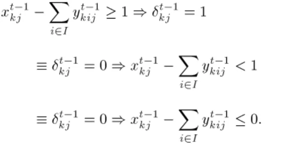
Simply, the contrapositive can be formulated in the mathematical optimization model as Relations (13) and (14). In order to impose the second side (C ) A_B), we utilize an auxiliary (indicator) variable t 1 kj
such that: t 1
kj = 1 , xt 1kj
X
i2I
yt 1
kij 1; (23)
which can be decomposed and rewritten as Eqs. (24) and (25).
t 1
kj = 1 ) xt 1kj
X
i2I
yt 1
xt 1 kj
X
i2I
yt 1
kij 1 ) t 1kj = 1: (25)
In order to reformulate Eq. (25) so as to be added to the mathematical optimization model, rst, we have to write the contrapositive.
xt 1 kj
X
i2I
yt 1
kij 1 ) t 1kj = 1
t 1
kj = 0 ) xt 1kj
X
i2I
yt 1 kij < 1
t 1
kj = 0 ) xt 1kj
X
i2I
yt 1
kij 0: (26)
The linearized formats of Eqs. (24) and (26) are added to the model as Constraints (15) and (16), respectively. Finally, after adding variable to the model as well as the related dependency constraints, we are ready to impose C ) A _ B on the model:
C ) A _ B
xt 1kj = 1)t 1kj = 1_ X
i2I
RLt kij= 1
!
xt
kj= 1 ) kjt 1+
X
i2I
RLt kij 1
t 1 kj +
X
i2I
RLt
kij xt 1kij: (27)
4.5. Determining length of each time period In order to determine an appropriate value for the length of each time period t 2 T , rst, we have to calculate the likelihood of having 0 or 1 phone calls per each time period. Assuming a Poisson distribution with parameter for the number of hourly emergency phone calls, the probability that 0 or 1 phone call is received in each time period can be calculated through Eq. (28).
p(0) + p(1) = e t+ te t= (1 + t)e t: (28)
For the small amounts of t, the estimated value, e tt 1 t, can be used. The length of time periods
should be small enough in order to assure that, in each time period, at most one emergency call is received. We assume that the probability of receiving 0 or 1 phone call is greater than or equal to 1 . Therefore:
(1 + t)(1 t) 1 ) 1 2t2 1 : (29)
Accordingly, the length of each time period should be less than or equal to p
. For instance, assuming
= 0:01 and = 2 calls/hour, the length of each
time period should be less than or equal to 3 minutes, i.e., 20 time periods are needed for a 1-hour planning horizon. According to the data, in busy time periods, 6 calls are received within an hour. Hence, considering a condence level of 99%, the length of each time period is assumed to be 1 minute.
5. Numerical example
In this section, a simple numerical example is solved in order to demonstrate the performance and to validate the proposed model. The example includes ve demand points, two emergency stations, three ambulances, and a time horizon of 120 minutes. Ten incidents are as-sumed to happen during the time horizon. Ambulances #1 and #2 are of the basic type, while ambulance #3 is of the advanced type. Serving time varies between 8 to 10 minutes. Each emergency station has a capacity of two ambulances. Standard response time is assumed equal to 10 minutes. Emergency stations are labeled from 1 to 2, and the demand points are labeled from 3 to 7. Time distances between the demand points and the emergency stations are shown in Table 1.
The numerical example is solved using OPL and CPLEX 12.6. In this example, the statuses of ambu-lances #1 to #3 during the time horizon are depicted in Figures 3 to 5. The status (vertical axis) is equal to 0 if the ambulance is not available, i.e., it is on its way to an emergency station or is on its way to be relocated at an emergency station. Otherwise, the status shows the position of the ambulance: 1-2 for emergency stations and 3-7 for demand points. For instance, ambulance #2 is unavailable between time periods 62 and 69 and is relocated at emergency station 6 afterwards.
Ambulance #1 is stationed at emergency sta-tion #1 from time periods 1 to 15. In time period 15, it is dispatched in order to respond to the incident at demand point #6 and in period 21, and it will serve demand point #6 for about 10 minutes. Then, it returns to emergency station #1 and will be stationed there in time period 37. It will remain at emergency station #1 from periods 37 to 47 and, then, will be dispatched to demand point #4. It is unavailable from periods 48 to 81, and it is stationed at emergency
Table 1. Time distances of the numerical example. Demand
point
Emergency station
1 2
3 15 9
4 5 10
5 10 3
6 6 9
Figure 3. Status of ambulance #1.
Figure 4. Status of ambulance #2.
Figure 5. Status of ambulance #3.
station #2 by period 72. Between periods 72 and 74, ambulance #1 is available at emergency station #2 and, then, is dispatched in period 74 to respond to demand point #3 and will be unavailable until time period 101. It will be stationed at emergency station #2 in period 102 and will stay there until period 117. Finally, it will be dispatched to demand point #7 in period 117. Figures 4 and 5 demonstrate the status of ambulances #2 and #3 and can be explained similarly. In order to better illustrate the solution to the numerical example, the assignment of ambulances to demands is illustrated in Table 2.
6. Sensitivity analysis
This section aims to investigate the eect of changing dierent parameters on the performance of the model. Three parameters have been considered to conduct the sensitivity analysis: number of emergency vehicles,
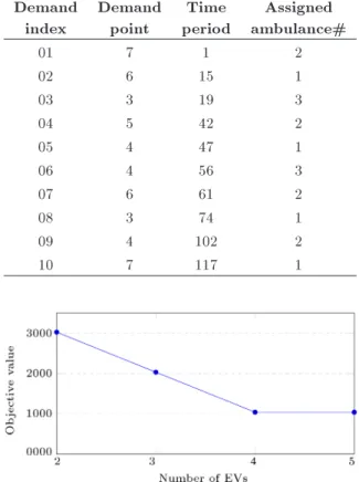
Table 2. Assignment of ambulances to demand points in the numerical example.
Demand index
Demand point
Time period
Assigned ambulance#
01 7 1 2
02 6 15 1
03 3 19 3
04 5 42 2
05 4 47 1
06 4 56 3
07 6 61 2
08 3 74 1
09 4 102 2
10 7 117 1
Figure 6. Objective value versus number of EVs.
service time, and standard response time. A small-size test problem, including 30 time periods, 3 emergency vehicles, 2 emergency stations, and 5 demand points, is utilized as the test bed for the analysis.
6.1. Changing the number of EVs
By increasing the number of ambulances from 3 to 4, the objective function is expected to improve. The results of this analysis are illustrated in Figure 6 and Table 3.
As shown in Figure 6, decreasing the number of ambulances down to 2 make the number of EVs inadequate for the whole demand coverage. Besides, increasing the number of ambulances to 4 and 5 results in a case in which only one incident remains uncovered and the objective function becomes better consequently. Adding one ambulance to the eet, we were not able to cover all the demands, which is a reason of limited capacity of emergency stations. Because the capacity of each station is equal to 2, thus relaxing emergency stations' capacity constraint (Eq. (2)), the objective function decreases down to 51. It means that with 5 ambulances at hand, we are able to cover all 6 incidents in this case.
6.2. Changing service time
In this subsection, we observe the behavior of the objective function while changing the value of service
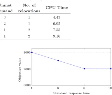
Table 3. Number of EVs sensitivity analysis. Max. no.
of EVs
Objective value
Unmet demand
No. of
relocations CPU Time
2 3024 3 1 4.43
3 2031 2 1 6.05
4 1039 1 2 7.55
5 1039 1 2 9.16
Figure 7. Objective value versus service time.
time. We expect the objective function to improve as a result of decreasing service time. Table 4 and Figure 7 depict the results of this sensitivity analysis.
As illustrated in Table 4, service time is decreased from 8 to 6; as a result, one unmet demand is covered in the new setting. By increasing this time to 10 and 12, the ambulances are not available in the rst time periods of the planning horizon. Therefore, they cannot be relocated for further demand coverage in upcoming periods.
6.3. Changing standard response time
In this subsection, standard response time, Tst, is
manipulated in order to observe the impact on the objective value. The objective value is expected to
Figure 8. Objective value versus standard response time.
increase/decrease in the same way as Tst. The results
are illustrated in Table 5 and Figure 8.
According to Figure 8, decreasing the standard response time from 8 down to 4 minutes causes 4 in-cidents to remain uncovered. Likewise, decreasing the standard response time to 6 minutes causes 3 incidents to be uncovered. On the other hand, increasing this parameter form 8 to 10 improves the objective value only by one unit from 2031 to 2030.
7. Computational Results
In this section, the ecacy of the proposed model is investigated using several simulated test cases. The
Table 4. Service time sensitivity analysis. Service
time
Objective value
Unmet demand
No. of
relocations CPU time
6 1039 1 2 6.00
8 2031 2 1 6.04
10 3013 3 0 5.99
12 3013 3 0 6.04
Table 5. Standard response time sensitivity analysis. Standard
response time
Objective value
Unmet demand
No. of
relocations CPU time
4 4011 4 1 6.03
6 3016 3 1 5.97
8 2031 2 1 5.96
test cases are generated and solved in small-, medium-, large-, and extra-large sizes.
Reviewing the literature, we found that there are was no problem set in order to be used as test cases of the model; hence, several test cases were simulated in dierent sizes. The instances vary in terms of the number of time periods in the planning horizon, number of EVs available, number of emergency sta-tions, and number of demand points. These articial test problems were created according to the following parameters:
Planning horizon T : 30, 60, 90, 120, 240;
Number of EVs E: 2, 3, 4, 5;
Number of emergency stations E: 2, 3, 4;
Number of demand points I: 5, 6, 7, 80.
For each instance, a hypothetical area of service is considered. This area is divided into several subareas. Number of the sub-areas equals that of demand points. Demand points are actually the center of these sub-areas. The demands are then distributed randomly in the whole area. Number of demands in each demand point equals that of demands happening in the respective sub-area. Each demand is associated with a type that is determined randomly, with a lower probability for severe incidents. The service time needed at each demand point is determined based on the ambulance type and demand type afterwards. The service times vary in the range of 8 to 12 minutes.
These instances will be referred to as: LRL-T-E-S-I, e.g., LRL-30-3-2-5 refer to a set of problems with 30 time periods, 3 emergency vehicles, 2 emergency stations, and 5 demand points. Three problems sets in three dierent sizes are considered: 20 small-size, 12 medium-size, and 8 large-size problems. The amount of total demand varies from 5 to 8 for small instances, from 9 to 11 for medium-size instances, and nally from 13 to 18 for large-size instances. It should be mentioned that although total demand is xed, the amount of demand in each time period is generated randomly. The locations of the demand points and stations are generated based on a uniform distribution. Assuming the speed of 50 km/h for the EVs, the time distance between the points is calculated afterwards. EV service times are assumed to be between 8 and 12 minutes based on the type of the EV. As mentioned before, the amount of unmet demand should be penalized in the objective function; = 1000 is considered as the penalty coecient. Standard response time, Tst, is
equal to 7 minutes for all the instances.
All the computations were carried out on an Intel® Q740 running at 1.73 GHz with up to 4 GB of
memory. The models are coded in Optimization Pro-gramming Language (OPL) and solved using CPLEX 12.6. A time limit of 3600 seconds was set for all
the test instances. The results are illustrated in Table 6. The rst and second columns represent the dimension and index of the problem in that dimension, respectively. The third column illustrates the best objective value found within the time limit, while the fourth column shows the number of relocations in the best solution. The unmet demand penalized in the objective function is shown in the fth column; nally, the sixth column shows the total CPU time for solving the problem.
According to the results of instances 1 to 20 (LRL-30-3-2-5), 86% of the demand is covered using the three available ambulances. Total demand in each instance of 1 to 10 is equal to 5 or 6. The increase in the amount of demand in instances 11-20 to 7 and 8 incidents has rendered the three available ambulance unable to cover all the demand, which is why the number of unmet demands is increased in these instances. In instances 1 to 10, the number of relocations is equal to 2, while this value is increased to 3 for instances 11 to 20, which seems to be predictable due to the increase in the demand. The CPU time for small-sized instances is 5.84 seconds on average, which is an acceptable duration for this size. The results of instances 21 to 32 (medium-size instances) show that 97.5% of the demands are covered. By increasing the number of incidents (demands) from 9 to 11, the four EVs available are not able to cover all the demands. The increase of the demand coverage compared to the small instances is a result of increment in the number of ambulances as well as the longer planning horizon. Furthermore, by increasing the amount of demand and the length of planning horizon, the number of relocations varies from 6 to 8. The average CPU time in this size varies and is approximately equal to 146 seconds, which seems to be a rational time for medium-size problems.
As illustrated in the table, in large-size instances, 100% of the demands are covered due to a reason similar to that mentioned before. The number of relocations varies within the range of 10 and 15 by increasing the number of time periods and the amount of demand.
In the extra-large instances (#41-55), the average demand coverage rate for the rst subcategory (#41-50) is about 90.75% and for the second category (#51-55) is 92.18%. The CPU time in the second category seems to be high. Therefore, one may consider presenting a solution method to reduce this time as a potential for future research.
8. Conclusion
This paper focused on emergency vehicle location and relocation problem with the purpose of dealing with emergency demands considering service time, response
Table 6. Test problems computational results.
Dimensions Instance# No. of demands
Obj. value
Tot. travel
time
Tot. relocation
time
Tot. unmet demand
cost
No. of relocations
No. of unmet demand
CPU time
LRL-30-3-2-5
1 10 22 18 4 0 2 0 6.01
2 10 18 14 4 0 2 0 6.59
3 10 26 18 8 0 2 0 6.12
4 10 23 15 8 0 2 0 6.00
5 10 23 15 8 0 2 0 6.01
6 12 2012 8 4 2000 2 2 6.12
7 12 24 18 6 0 3 0 6.03
8 12 1026 18 8 1000 2 1 6.07
9 12 1023 15 8 1000 2 1 5.92
10 12 29 20 9 0 3 0 6.26
11 14 1021 15 6 1000 3 1 6.00
12 14 1024 18 6 1000 3 1 6.07
13 14 2018 14 4 2000 2 2 6.04
14 14 1028 19 9 1000 3 1 6.35
15 14 1029 20 9 1000 3 1 6.32
16 14 1024 18 6 1000 2 1 6.16
17 16 2024 18 6 2000 3 2 6.04
18 16 3018 14 4 3000 2 3 7.75
19 16 2028 19 9 2000 3 2 5.98
20 16 2024 18 8 2000 3 2 5.78
LRL-60-4-3-6
21 9 40 25 15 0 6 0 168.07
22 9 53 29 24 0 7 0 168.79
23 9 55 34 21 0 6 0 168.56
24 9 1038 21 17 1000 6 1 169.01
25 10 49 29 20 0 7 0 165.28
26 10 57 31 26 0 8 0 182.39
27 10 63 42 21 0 6 0 174.15
28 11 1042 25 17 1000 6 0 167.15
29 11 1051 32 19 1000 6 1 169.13
30 11 54 34 20 0 7 0 167.96
31 11 63 34 29 0 8 0 172.64
32 11 69 45 24 0 7 0 167.73
LRL-90-5-4-7
33 13 62 36 26 0 10 0 1570.91
34 15 78 44 34 0 12 0 1570.91
35 16 84 47 37 0 13 0 1768.99
36 17 95 55 40 0 14 0 1787.65
37 18 102 57 45 0 15 0 1883.80
38 19 92 53 39 0 14 0 1831.77
39 18 93 52 41 0 15 0 2083.07
Table 6. Test problems computational results (continued).
Dimensions Instance# No. of demands
Obj. value
Tot. travel
time
Tot. relocation
tim e
Tot. unmet demand
cost
No. of relocations
No. of unmet demands
CPU time
LRL-120-3-2-80
41 12 89 43 46 0 12 0 632.74
42 12 1089 42 47 1000 11 1 637.92
43 12 107 51 56 0 12 0 626.87
44 12 2074 37 37 2000 9 2 653.14
45 12 1090 44 46 1000 11 1 645.98
46 14 1098 49 49 1000 12 1 647.47
47 14 1109 53 56 1000 13 1 672.91
48 14 1113 57 56 1000 12 1 637.89
49 14 3078 39 39 3000 10 3 638.29
50 14 2087 47 40 2000 11 2 636.28
LRL-240-3-2-80
51 24 178 86 92 0 24 0 4816.44
52 24 4152 76 76 4000 19 4 4962.41
53 24 2180 88 92 2000 22 2 4801.36
54 28 2205 104 101 2000 25 2 4905.01
55 28 2218 106 112 2000 26 2 5065.19
time, and return time. The proposed mathematical optimization model is a multi-period model taking into account real-time conditions. To the best of our knowledge, for the rst time, a model with the considerations mentioned in Sections 3 and 4 is pre-sented in this paper. The model aims to minimize response times as well as ambulance relocations in order to cover as much demand as possible taking into account the resource limitations (emergency vehicles). A sensitivity analysis was designed and conducted in order to validate the presented model. The values of three dierent parameters, namely number of available EVs, service time, and standard response time, were manipulated so as to observe the impact on the ob-jective value. For the purpose of model evaluation, a set of test problems was generated to solve using OPL and CPLEX 12.6 in 4 sizes: small-sized, middle-sized, large-sized, and extra-large-sized cases. The results show the ecacy of the proposed model. According to the outcome of the computational results, it can be concluded that increasing the length of planning horizon or number of available EVs increases the number of ambulance relocations, resulting in a higher response to demand percentage. The model could be solved in a rational time in small-, middle- and large-sized instances, whilst, in the extra-large-size test prob-lems, the average solution time was higher relatively. Although many new aspects of the real-world problem were considered in this modeling, still some issues need to be studied in the future. For example, including hospitals in the problem formulation and dividing
the unavailability time into intervention time at the scene and travel time to the hospital provides better modeling of real-world situations. Besides, due to the uncertainty in the demand of each time period and EV service time, taking these uncertainties into account enables us to produce more reliable solutions in real-world applications. As mentioned before, in large-sized instances, the solution time is not acceptable compared to the planning horizon; therefore, presenting special solution methods for the problem can be seen as a potential future research.
References
1. Pons, P.T., Haukoos, J.S., Bludworth, W., Cribley,
T., Pons, K.A., and Markovchick, V.J. \Paramedic response time: does it aect patient survival?", Aca-demic Emergency Medicine, 12(7), pp. 594-600 (2005).
2. Peng, Q. and Afshari, H. \Challenges and solutions
for location of healthcare facilities", Ind Eng and Manage, 3(2), pp. 127-138 (2014). DOI: 10.4172/2169-0316.1000127
3. Brotcorne, L., Laporte, G., and Semet, F. \Ambulance
location and relocation models", European Journal of Operational Research, 147(3), pp. 451-463 (2003).
4. Henderson, S.G. \Operations research tools for
ad-dressing current challenges in emergency medical ser-vices", Wiley Encyclopedia of Operations Research and Management Science (2011).
5. Li, X., Zhao, Z., Zhu, X., and Wyatt, T. \Covering
response facility location and planning: a review", Mathematical Methods of Operations Research, 74(3), pp. 281-310 (2011).
6. Rais, A. and Viana, A. \Operations research in
healthcare: a survey", International Transactions in Operational Research, 18(1), pp. 1-31 (2011).
7. Caunhye, A.M., Nie, X., and Pokharel, S.
\Opti-mization models in emergency logistics: A literature review", Socio-Economic Planning Sciences, 46(1), pp. 4-13 (2012).
8. Farahani, R.Z., Asgari, N., Heidari, N., Hosseininia,
M., and Goh, M. \Covering problems in facility loca-tion: A review", Computers & Industrial Engineering, 62(1), pp. 368-407 (2012).
9. Aringhieri, R., Bruni, M.E., Khodaparasti, S., and van
Essen, J. \Emergency medical services and beyond: Addressing new challenges through a wide literature review", Computers & Operations Research, 78, pp. 349-368 (2017).
10. Toregas, C., Swain, R., ReVelle, C., and Bergman, L.
\The location of emergency service facilities", Opera-tions Research, 19(6), pp. 1363-1373 (1971).
11. Church, R. and Velle, C.R. \The maximal covering
location problem", Papers in Regional Science, 32(1), pp. 101-118 (1974).
12. Eaton, D.J., Daskin, M.S., Simmons, D., Bulloch, B.,
and Jansma, G. \Determining emergency medical ser-vice vehicle deployment in Austin, Texas", Interfaces, 15(1), pp. 96-108 (1985).
13. Schilling, D., Elzinga, D.J., Cohon, J., Church, R., and
ReVelle, C. \The team/eet models for simultaneous facility and equipment siting", Transportation Science, 13(2), pp. 163-175 (1979).
14. Hogan, K. and ReVelle, C. \Concepts and applications
of backup coverage", Management Science, 32(11), pp. 1434-1444 (1986).
15. Daskin, M.S. \A maximum expected covering location
model: formulation, properties and heuristic solution", Transportation Science, 17(1), pp. 48-70 (1983).
16. Repede, J.F. and Bernardo, J.J. \Developing and
validating a decision support system for locating emergency medical vehicles in Louisville, Kentucky", European Journal of Operational Research, 75(3), pp. 567-581 (1994).
17. Goldberg, J., Dietrich, R., Chen, J.M., Mitwasi, M.G.,
Valenzuela, T., and Criss, E. \Validating and applying a model for locating emergency medical vehicles in Tuczon, AZ", European Journal of Operational Re-search, 49(3), pp. 308-324 (1990).
18. ReVelle, C. and Hogan, K. \The maximum availability
location problem", Transportation Science, 23(3), pp. 192-200 (1989).
19. Ball, M.O. and Lin, F.L. \A reliability model applied
to emergency service vehicle location", Operations Research, 41(1), pp. 18-36 (1993).
20. Rajagopalan, H.K., Saydam, C., and Xiao, J. \A
multiperiod set covering location model for dynamic redeployment of ambulances", Computers & Opera-tions Research, 35(3), pp. 814-826 (2008).
21. Degel, D., Wiesche, L., Rachuba, S., and Werners,
B. \Time-dependent ambulance allocation consider-ing data-driven empirically required coverage", Health Care Management Science, 18(4), pp. 444-458 (2015).
22. Jagtenberg, C., Bhulai, S., and van der Mei, R. \An
ecient heuristic for real-time ambulance redeploy-ment", Operations Research for Health Care, 4, pp. 27-35 (2015).
23. Gendreau, M., Laporte, G., and Semet, F. \A dynamic
model and parallel tabu search heuristic for real-time ambulance relocation", Parallel Computing, 27(12), pp. 1641-1653 (2001).
24. Kolesar, P. and Walker, W.E. \An algorithm for
the dynamic relocation of re companies", Operations Research, 22(2), pp. 249-274 (1974).
25. Gendreau, M., Laporte, G., and Semet, F. \Solving an
ambulance location model by tabu search", Location Science, 5(2), pp. 75-88 (1997).
26. Yang, S., Hamedi, M., and Haghani, A. \Online
dispatching and routing model for emergency vehicles with area coverage constraints", Transportation Re-search Record: Journal of the Transportation ReRe-search Board, 1923, pp. 1-8 (2005).
27. Maxwell, M.S., Restrepo, M., Henderson, S.G., and
Topaloglu, H. \Approximate dynamic programming for ambulance redeployment", INFORMS Journal on Computing, 22(2), pp. 266-281 (2010).
28. Nogueira Jr, L., Pinto, L., and Silva, P. \Reducing
emergency medical service response time via the reallo-cation of ambulance bases", Health Care Management Science, 19(1), pp. 31-42 (2016).
29. Schmid, V. \Solving the dynamic ambulance relocation
and dispatching problem using approximate dynamic programming", European Journal of Operational Re-search, 219(3), pp. 611-621 (2012).
30. Knight, V.A., Harper, P.R., and Smith, L.
\Ambu-lance allocation for maximal survival with heteroge-neous outcome measures", Omega, 40(6), pp. 918-926 (2012).
31. Belanger, V., Kergosien, Y., Ruiz, A., and Soriano, P.
\An empirical comparison of relocation strategies in real-time ambulance eet management", Computers & Industrial Engineering, 94, pp. 216-229 (2016).
32. Enayati, S., Mayorga, M.E., Rajagopalan, H.K., and
ap-proach to improve service coverage with fair and restricted workload for ems providers", Omega, 79, pp. 67-80 (2017). https://doi.org/10.1016/j.omega. 2017.08.001
33. Yue, Y., Marla, L., and Krishnan, R. \An ecient
simulation-based approach to ambulance eet alloca-tion and dynamic redeployment", In AAAI (2012).
34. Alanis, R., Ingolfsson, A., and Kolfal, B. \A Markov
chain model for an ems system with repositioning", Production and Operations Management, 22(1), pp. 216-231 (2013).
35. Sudtachat, K., Mayorga, M.E., and Mclay, L.A. \A
nested-compliance table policy for emergency medical service systems under relocation", Omega, 58, pp. 154-168 (2016).
36. Van Barneveld, T.C., Bhulai, S., and van der Mei, R.D.
\A dynamic ambulance management model for rural areas", Health Care Management Science, 20(2), pp. 165-186 (2017). ISSN 1572-9389.
37. Majzoubi, F., Bai, L., and Heragu, S.S. \An
op-timization approach for dispatching and relocating ems vehicles", IIE Transactions on Healthcare Systems Engineering, 2(3), pp. 211-223 (2012).
38. Lei, C., Lin, W.H., and Miao, L. \A stochastic
emergency vehicle redeployment model for an eective response to trac incidents", IEEE Transactions on Intelligent Transportation Systems, 16(2), pp. 898-909 (2015).
39. Schmid, V. and Doerner, K.F. \Ambulance location
and relocation problems with time-dependent travel times", European Journal of Operational Research, 207(3), pp. 1293-1303 (2010).
40. Saydam, C., Rajagopalan, H.K., Sharer, E., and
Lawrimore-Belanger, K. \The dynamic redeployment coverage location model", Health Systems, 2(2), pp. 103-119 (2013).
41. Naoum-Sawaya, J. and Elhedhli, S. \A stochastic
optimization model for real-time ambulance redeploy-ment", Computers & Operations Research, 40(8), pp. 1972-1978 (2013).
Biographies
Saeed Firooze received his BSc degree in Rail Trans-portation Engineering from Iran University of Science and Technology (IUST), Tehran, Iran, and his MSc degree in Socioeconomic Systems Engineering from Sharif University of Technology, Tehran, Iran in 2013 and 2016, respectively. His main areas of interest are integer programming, mathematical modeling, and health-care systems optimization.
Majid Raee received his BSc degree in Industrial Engineering from Isfahan University, Isfahan, Iran in 2003, and his MSc and PhD degrees in Industrial En-gineering from Sharif University of Technology, Tehran, Iran in 2006 and 2013, respectively. In 2013, he joined the Department of Industrial Engineering at Sharif University of Technology, Tehran, Iran, as an Assistant Professor. Dr. Raee's research interests include stochastic programming, operations research, mathematical programming, quality management, and quality control.
Seyed Mohammad Zenouzzadeh received his BSc degree in Rail Transportation Engineering from Iran University of Science and Technology (IUST), Tehran, Iran. He is currently an MSc student in Socioeconomic Systems Engineering at University of Tehran, Tehran, Iran. His main research interests include integer pro-gramming, design and implementation of algorithms, combinatorial optimization, and network design and optimization.