Studying the impact of quantity discount contract and cost-sharing contract on a two-echelon green supply chain profit

(1)

Studying the impact of quantity discount contract and cost sharing

contract on a two-echelon green supply chain profit

Ata Allah Taleizadeh

1*

_{, Naghmeh Rabie}

2

1

School of Industrial Engineering, College of Engineering, University of Tehran, Tehran, Iran

2_{School of Industrial Engineering, Islamic Azad University, South Tehran Branch}

[email protected], [email protected]

Abstract

The members of a chain always try to find new ways in order to raise their profit. Hence we intend to study two different scenarios in a single item two-echelon green supply chain including two manufacturers and one retailer to study the effects of two effective contracts on members’ profit. Two scenarios are discussed and in first one, first manufacturer proposes quantity discount contract to retailer and in second scenario retailer proposes cost sharing contract to second manufacturer. Then a numerical example and sensitivity analysis is implemented to review the mathematical relations in detail and assess the effect of some parameters on our decision variables and profits. The results show that cost sharing contract is more beneficial for retailer and second manufacturer than quantity discount contract.

Key words:

green supply chain, greening level, quantity discount, cost sharing

1-Introduction and literature review

Using contracts is so prevalent between businesses and companies. There are different kinds of contracts which are employed considering different conditions. Quantity discount and cost sharing are two helpful and utilized contracts which are widely used in recent years and they are common among manufacturer and retailer. Quantity discount contract is dependent on amount of products which customers purchase and in addition to raising sales amount, it causes to decrease operational costs. Increasing customers shopping induces to receive more discounts from manufacturer. Cost sharing contract which is employed in this paper, is another useful contract that helps managers to improve and coordinate their businesses. In cost sharing contract retailer incurs some part of manufacturer’s cost if he/she considers lower wholesale price for retailer. The purpose of this paper is to study the impact of these contracts on members’ profit in a green supply chain and assist managers to decide how to coordinate their businesses.

*_{Corresponding Author}

Journal of Industrial and Systems Engineering

Vol. 11, No. 1, pp. 24-49

Winter (January) 2018

(2)

In two scenarios we check the effect of each contract on profits. Nowadays human consumes wide range of products. In order to save our environment we can make our supply chains green instead of traditional supply chains. Thus many authors and researchers studied and worked on this issue. For example: Basiri and Heydari (2017) delved the green channel coordination in a two-stage supply chain. In this supply chain beside non-green traditional product, sustainable green product was planned to produce. Retailer decided for sales effort level and retail price of the green product. On the contrary, manufacturer decided for product green quality. Heydari and et al. (2017) investigated a two-echelon reverse supply chain (RSC) including one manufacturer and one retailer. They intended to increase customers’ willingness to bring back used products by proposing discount or a direct fee in exchange for returning end-of-life (EOL) products. They also extended their model by considering a closed loop supply chain (CLSC). Xie and et al. (2017) studied dual-channel closed-loop supply chains and reviewed coordination of centralized and decentralized decision making process. They applied revenue sharing mechanism and assessed the relationship among the recycle rate and the recycle revenue sharing ratio. Hassanzadeh-Amin and et al. (2017) considered forward and reverse supply chains in a closed-loop supply chain (CLSC) network. They proposed a tire remanufacturing in this CLSC network in order to maximize total profit. Paydar and et al. (2017) examined a closed-loop supply chain (CLSC) and explained that manufacturers encounter many challenges and they look for different methods to have more efficient production system. Therefore they introduced a proper approach for solving resource limitation which is one of the most important challenges for manufacturers. Finally recycling used products was proposed to assist them to make their production system more effective. As it is clear, all organizations and businesses have a unique goal which is maximizing profit. But for achieving their goal they would be faced with lots of challenges. So they always look for different methods or policies to increase their profit. Recently applying contracts has been so common and useful between managers. Because using different contracts, not only increase and raise the profit of organizations, but also assist them to coordinate their organizations and act more efficiently. So in this paper two contracts called quantity discount and cost sharing are studied to give managers managerial insight and it can help them to decide more accurately.

One of the ways of trading off in different businesses is presenting discount to buyer. There are several reasons and purposes for presenting discount in different businesses, e.g. attracting more customers, increasing amount of customers buying, changing customers shopping behavior and etc. The first contract which is used in this research is quantity discount. This contract causes higher profit and also costs reduction like set up, operational and holding costs. This contract which is established between the retailer and manufacturer, depends on products quantities which retailer purchases. By purchasing more products, retailer will receive more discounts from manufacturer. In recent years many researchers have studied this contract and used it in their researches. For example: Chaharsooghi and et al (2011) considered a two-stage supply chain with lead times and stochastic demand. They studied coordination of reorder point and order quantity at the same time. The presented model caused global optimization of order quantity–reorder point decisions and the proposed model caused to coordinate the channel and the coordination of both decisions induced to increase profit of supply chain. Heydari (2014) reviewed the coordination of a buyer-seller supply chain which contains order size constraint. The seller for convincing the buyer to optimize its safety stock, proposed a time-based short-term price discount in every replenishment cycle. Maximum and minimum discounts which were admissible for both parties are assessed and a proper discount schedule is concluded. Heydari and Norouzinasab (2015) studied a two-echelon supply chain and proposed a discount model for coordinating pricing and ordering decisions. Quantity discount as a coordination mechanism was proposed for coordinating pricing and ordering decisions at the same time. From two aspects the discount policy was defined: (1) marketing viewpoint (2) operations management viewpoint. The results indicated that the specified policy can coordinate supply chain and increase profitability of supply chain and also all supply chain members with respect to decentralized condition. . Heydari and Norouzinasab (2016) applied an incentive policy for coordinating pricing, ordering and lead time in a two-echelon supply chain. Demand was considered stochastic and depended on price and lead time. They presented a game-theory approach to review members’ decision making process. Applying the proposed approach induced to increase whole

(3)

supply chain and both members profitability. Nie and Du (2017) delved quantity discount contract in a two-echelon supply chain including two retailers and one supplier. Both retailers sell a product produced by a same supplier. The supplier proposes an equal quantity discount contract to both retailers by defining the best wholesale price to maximize the profit of both games and retailers should choose best retail price to maximize their profit. Additionally quantity discount is combined with given fees to coordinate the supply chain. Jiao and et al. (2017) studied the stochastic lot-sizing model with quantity discounts. By each order, an all-unit quantity discount is utilized based on the ordered quantities. Tamjidzad and Mirmohammadi (2017) consider a (r,Q) model which is single item with confined resource and rising quantity discount whereas demand is discontinuous and stochastic. Bohner and Minner (2016) studied a supply chain model with synchronous supplier selection and order allocation for multiple items. The supplier proposes quantity and business volume discounts and they are exposed to failure. They also remarked all-units and rising quantity discounts and they tried to find best solutions by mixed-integer linear programming. Munson and Hu (2010) assessed some methods to compute best order quantities and total purchasing and inventory costs whereas quantity discount was executed for pricing the products. The methods for quantity discount schedule are prepared for four various strategic purchasing scenarios.

Alfares and Turnadi (2016) presented quantity discounts and backordering of shortages for a single product lot-sizing model with several suppliers. Zissis and et al. (2015) studied a two-echelon supply chain consisting of a manufacturer and a retailer with private information. The manufacturer proposed quantity discount contract to retailer in order to reduce their costs. Mahdavi-Mazdeh and et al. (2015) considered a dynamic lot-sizing model with supplier selection in a single item supply chain. They divided their model into two parts and they studied quantity discount in second part. Partha-Sarathi and et al. (2014) extended a model by combing quantity discount contract and revenue sharing for supply chain coordination that it was beneficial for members of supply chain. Alfares and Ghaithan (2016) presented an inventory model whereas demand rate and holding cost were considered fixed. They expressed that for higher quantity order, using quantity discount contract causes less purchase cost. Çebi and Otay (2016) expressed that supplier selection is one of the main decisions in organizational competitiveness. They considered a two-stage fuzzy approach which was a multi-product, multi-supplier problem with several objectives. It modeled by quantity discount and other factors. Chang and et al. (2010) studied a three-echelon supply chain consisting of a supplier, a vender and multi retailer. They believed that quantity discount can be used as a coordination structure between all parties. Considering the results, this coordination caused to reduce total costs. Lau and et al. (2008) did not focus only on this matter that manufacturer should design quantity discount in order to impel retailer to order in larger quantities. They considered handling-charge reduction procedure in addition to quantity discount. To maximize the manufacturer’s profit, they developed their model for designing quantity discount and handling-charge reduction. Jackson and Munson (2016) offered quantity discount to identify the best warehouse capacity level for multiple products. Burke and et al. (2008) considered a provision issue whereas quantity discount was offered by supplier. It resulted in minimizing the summations of separable concave functions.

In second scenario cost sharing contract is designed. This contract is so practical and useful for managers. Because by sharing the costs between retailer and manufacturer they can act more coordinated. Cost sharing contract helps manufacturer to produce more products, so retailer can satisfy more customer’s demand. Thus both members can increase their profitability. Considering the importance and application of this contract many scientists and researchers have delved and considered this contract in their studies. For example: Lee and et al. (2016) evaluated vendor-managed inventory (VMI) models with stockout-cost sharing which was signed up between supplier and customer. They also proved that VMI and stockout-cost sharing can cause supply chain coordination despite of the supplier's reservation cost. Ghosh and Shah (2015) considered supply chain coordination models caused by green supply chain improvisation. They modeled cost sharing contract and studied the effect of this contract on green supply chain. Avni and Tamir (2016) considered a usual cost-sharing scheduling game. The game distributed unit cost sharing games with weighted players. Zhou and et al. (2016) reviewed a low-carbon supply chain consisting of one manufacturer and one retailer. They explained how to perfect the supply chain performance by designing contracts. They used the co-op advertising and emission reduction cost sharing contracts and showed that

(4)

these contracts caused supply chain coordination and win-win condition. Roma and Perrone (2016) delved the impact of outcome-based versus ex ante-based cost-sharing contract regarding competition of companies’ profitability. They described that outcome-based mechanisms happened by optimal cost sharing mechanisms.

Ovaskainen and et al. (2017) checked that whether cost sharing causes extra private investments or it exchanges explicit funds for private capitals. The results showed that applying cost sharing is lucrative in a balanced policy mix. Chao and et al. (2009) studied two contracts whereas recall costs was shared between manufacturer and supplier in order to improve products quality. In first contract they reviewed cost sharing which was based on optional root and in second contract they examined partial cost sharing based on whole root. They illustrated that applying both contracts was useful for them and also first contract induced higher profits for the supply chain and the manufacturer. Leng and Parlar (2010) studied an assembly supply chain including one manufacturer and multiple suppliers. They applied cost sharing contact in order to coordinate their assembly supply chain. So manufacturer’s and all suppliers’ profit were increased. Chalkley and Malcomson (2002) studied a health service supplying whereas cost sharing contract was applied to reduce the total costs. Zhao and et al. (2014) evaluated the coordination of logistics service supply chain containing of one service integrator and one supplier, by applying cost sharing contract. This contract induced the sales to increase by providing the renown of the supply chain and also increased the profits of both members and the entire supply chain. Also some related works can be found in Taleizadeh et al. (2008a,b, 2009, 2010a,b, 2011, 2013a,b, 2014).

Although many researchers and authors reviewed these issues and applied these contracts in their papers, none of them have considered quantity discount and cost sharing contracts together in a two-echelon green supply chain including two manufacturers and one retailer. Thus in this paper we consider a green supply chain and we intend to study the impact of these two contracts on member’s profit.

2- Problem description

In this study a single item two-echelon green supply chain including two manufacturers and one retailer is considered. Both manufacturers produce green products and customers are looking for them. Green products are kind of goods which are biodegradable and they do not harm the environment and they avoid pollution. Thus, in order to satisfy customers’ demands, retailer purchases green products from both manufacturers and they sell their products by retailer. We consider two scenarios via two contracts to make an inventory model for a two-echelon green supply chain. In first scenario quantity discount contract is designed between retailer and first manufacturer. This manufacturer in order to increase its sales proposes this contract to retailer and considers given discount for him/her. Actually retailer by purchasing specified amount of green products can be endowed special amount of this discount. In this contract manufacturer incurs the greening cost. In second scenario retailer is faced with higher wholesale price, and second manufacture incurs higher greening cost with respect to first scenario. Therefore retailer in order to incur lower wholesale price, offers cost sharing contract to second manufacturer to share greening cost. Due to sharing greening cost between retailer and second manufacturer, the manufacturer incurs lower greening cost and can increase his/her profit. So utilizing this contract would be useful for both members which we will more discuss about it in the following.

The notations of this study are as follows: Decision variables:

*

:

DC

q The optimal order quantity by retailer under decentralized condition

*

:

C

q

The optimal order quantity under centralized condition

*

:

DC

p

The optimal selling price for retailer under decentralized condition

*

:

C

(5)

Parameters:

D

r

Demand



Green elasticity of products (0  1, 1 ).



Price elasticity of products ( 1).

a

Population of green products customers.

Y Wholesale price per unit of product.

r

A

Retailer’s ordering cost per order.

r

h

Retailer’s holding cost per unit of product.

M

A

Manufacturer’s ordering cost per order.

M

h

Manufacturer’s holding cost per unit of product.

C

_ Greening cost.



Product greening level.

p

C

Production cost per unit of product.

d Coefficient of discount under quantity discount contract.



The percentage of sharing greening cost under cost sharing contract.

'

Y Wholesale price per unit of product under cost sharing contract ( 'Y Y).

M



Manufacturer’s profit function in unit of time.

r



Retailer’s profit function in unit of time.

SC

 Supply chain profit function in unit of time.

The assumptions of this research are as follows:

1. Our supply chain consists of two manufacturers and one retailer.

2. Both manufacturers produce green products.

3. This supply chain is single item and only one type of green products is produced.

4. Demand function is nonlinear and depends on price and product greening level.

5. In first scenario manufacturer proposes quantity discount contract to retailer.

6. In second one retailer offers cost sharing contract to second manufacture.

7. Leakage is not permitted.

3-Mathematical model

Profit functions of supply chain and the members of chain in a two-echelon supply chain which includes two manufacturers and one retailer are described in this section and we will explain them. In this research demand function is nonlinear and it depends on price and product greening level which is as follows:

( , )

D

r

p





ap

 



(1)

Now we will demonstrate the profit functions of supply chain and two manufacturers and the retailer. The profit function of retailer is as follows:

( , )

( , ) ( , ) ( , ) ( )

2

D

r D D r r

r p q

p q pr p Yr p A h

q 

(6)

In equation (2) pr_D( , )p represents annual retailer’s income and Yr_D( , )p shows annual purchasing

cost from manufacturer. ( D( , ))

r r p A q  and 2 r q

h respectively indicates annual ordering cost and annual

holding cost. The proof of concavity of retailer’s profit function is discussed in appendix (A). The first manufacturer’s profit function is as follows:

1

1 1 1 1 1 1 1

1 1 1 1 ( , ) ( , ) ( , ) ( ) ( , ) 2 D

M D M P D M

r p q

p q Y r p A C C r p h

q 



         (3)

And the second manufacturer’s profit function is shown with following equation:

2

2 2 2 2 2 2 2

2 2 2 2 ( , ) ( , ) ( , ) ( ) ( , ) 2 D

M D M P D M

r p q

p q Y r p A C C r p h

q 



         (4)

In both above equations ((3) and (4)) Yr_D( , )p indicates annual manufacturers’ income. Manufacturer’s

annual ordering cost and annual holding cost are respectively assessed by ( D( , ))

M r p A q  and 2 M q

h . As we

mentioned, both manufacturers produce green products and C_ shows greening cost and C r_{P D}( , )p

indicates production cost. Actually the formulas of profit function for both manufacturers are the same. But we will see the difference between them in numerical example and sensitivity analysis. In order to ease our model, we omitted the subscript of these two profit function and in the following we represent both

manufacturer’ profit function with_M( , )p q .

Finally the supply chain profit is generally calculated by following equation: ( , )

( , ) ( ) ( ) ( , )

2

D

SC r M D r M r M P D

r p q

pr p A A h h C C r p

q 



             (5)

This profit chain same as retailer’s profit function is concave and it is proved in appendix (B). In a chain, members can make decentralized or centralized decisions, based on different circumstance. In a decentralized decision making process each member make a decision individually for maximizing profit or minimizing cost. In the other hand in centralized decision making process a member as a leader makes a decision for profit or cost of chain.

In decentralized decision making process, optimal values of price and order quantity are assessed by retailer. In the following we will explain the calculation of optimal values of price and order quantity in decentralized condition.

For calculating price and order quantity in decentralized condition we use retailer’s profit function. So for finding these values we derive retailer’s profit function with respect to price and order quantity which are shown below:

1

( , )

0 (

(

)) 0

r

p

_ap

_{p Y}

A

r

p

q

   







_

_

 

_



_{ }

_

_{ }

_



(6)

By above equation, the value of P in decentralized and in unclosed-form condition is calculated which

is as follows:

( ) ( ) 1 r DC A Y q p q



   (7)

(7)

2

0

2

r

_ap

A

r

h

r

q

 





_



_{ }

_

_



(8) And also above equation (equation (8)) indicates that retailer’s profit function is derived with respect to

q and we can calculate the value of q in decentralized and in unclosed-form condition, which is as follows:

2 ( ) DC r r aA p q p h  

_



 (9)

Optimal value of P under decentralized condition is calculated in Eq. (10), by substituting

q

DC

( )

p

from

equation (9) into equation (7) and by substituting DC

p

from equation (10) into equation (9) optimal value

of q is assessed in equation (11):

*

1

DC

Y

p







(10)

* 2 r( 1)

DC r Y aA q h  



_



   (11)

After calculation of these decentralized values, supply chain profit and retailer’s and manufacturer’s profit function are obtained by substituting optimal values under decentralized condition in profit functions which are explained in the following.

Retailer’s profit function under decentralized condition which is represented by DC

( , )

* *

r

p q



is given in

following equation: * * * * * * * * ( , ) ( , ) ( , ) ( , ) ( ) 2 DC DC

DC DC DC DC D

r D D r _DC r

r p q

p q p r p Yr p A h

q













  (12)

Manufacturer’s profit function under decentralized condition which is represented by DC

( , )

* *

M

p q



is

obtained by following equation:

* * * * * * * ( , ) ( , ) ( , ) ( ) ( , ) 2 DC DC

DC DC D DC

M D M _DC P D M

r p q

p q Yr p A C C r p h

q 



        (13)

By summation of equation (12) and equation (13) profit chain under decentralized condition is obtained which is as follows:

* * * * * * ( , ) ( , ) ( ) ( ) ( , ) 2 DC DC

DC DC DC DC DC D DC

SC r M D r M _DC r M P D

r p q

p r p A A h h C C r p

q 



            (14)

Versus there is centralized decision making process whereas optimal values of price and order quantity are assessed by the leader. For finding these values, supply chain profit function should be derived with respect to price and order quantity. These calculations are shown below:

1

0 (

)(

) 0

SC r M

P

A

ap

p

C

p

q

   





_

_

 

_



_{ }

_



_

_



(15)

Optimal value of P under centralized and unclosed-formed condition is calculated by above equation

which is as follows:

( ) ( ) 1 r M P C A A C q p q



 _   (16)

Now we derive chain profit with respect to order quantity and then show the optimal value of order quantity under centralized and unclosed-formed condition, which are as follows:

(8)

2

(

)(

)

0

2

SC

A

r

A

M

ap

h

r

h

M

q

 









_{ }



_



_



(17)

2( )( )

( )

C r M

r M

A A ap

q p h h  

_

    (18)

By substituting equation(18) into equation (16), optimal value of p in centralized condition is generated

which is as follows: *

1

C

P

p







(19) And then by substituting equation (19) into equation (18) the optimal value of order quantity in centralized condition is calculated which is shown in below equation:

*

2(

)( (

1 )

)

P

r M

C

r M

C

A

a

q

h

 



_













(20)

Profit chain under centralized condition which is represented by C

( , )

* *

SC

p q



is obtained from following

equation: * * * * * * * * ( , ) ( , ) ( , ) ( ) ( ) ( , ) 2 C C

C C C D C

SC D r M _C r M P D

r p q

p q p r p A A h h C C r p

q 



          (21)

3-1- First scenario: Quantity discount contract

In this section we introduce and design quantity discount contract whereas first manufacturer propose it to retailer. Manufacturer consider discount for retailer if he/she purchases more green products from manufacturer. Thus quantity of purchasing green products is one of important factors in this contract. Applying this contract causes higher profit for retailer rather than decentralized condition. So the first necessary and sufficient condition from retailer point of view for agreement of quantity discount contract is as follows:

* * * *

( C , C , ) ( DC , DC )

r p q d r p q







(22)

Considering above equation retailer’s profit function under this contract is as follows:

* * * * * * * * ( , ) ( , , ) ( , ) ( , ) 2 C C

C C C C C D

r D D r _C r

r p q

p q d p r p dYr p A h

q 

       (23)

By substituting equation (23) and equation (12) into equation (22) we have following relations:

* * * * * * * * * * ( , ) ( , ) ( ) ( , ) ( ) ( , ) 2 2

C C DC DC

C C D DC DC D

D r _C r D r _DC r

r p q r p q

p dY r p A h p Y r p A h

q q

 

       (24)

In order to find the value of discount ( )d we have to solve above inequality:

* * * * * * * * * * * * ( , ) ( , ) ( , ) ( , ) 2 ( , ) ( , ) 2 C C

C C C D DC DC

D D r _C r D

DC DC

DC D

D r _DC r

r p q

dYr p p r p A h p r p

q

r p q

Yr p A h

q              (25)

In the following we have:

* * * * * *

*

* * * * * * *

( , ) ( , ) ( , ))

2 ( , ) ( , ) ( , ) ( , ) 2 ( , )

C DC DC DC DC DC

C

r r D D r D r

C C C C C DC C

D D D D D

A h q p r p r p A r p h q

p d

Y Yq Yr p Yr p r p Yr p q Yr p

  

    

(9)

So the upper threshold of d which is represented with

d

_max is as follows and it indicates the first necessary and sufficient condition from retailer point of view:

* * * * * * *

*

* * * *

* * *

max

2 ( , ) 2 ( , ) 2 ( , )

2 ( , )

( ( , )) ( ( , ))

( , )

C C C DC DC DC DC

D r D D r

C D

DC C C DC

r D r D

C DC C D

p r p h q p r p Yr p h q

d

Yr p

A q r p q A r p

Yq q r p

               (27)

Now we describe second necessary and sufficient condition which is from manufacturer point of view for participating in this contract. This condition expresses that manufacturer’s profit function under quantity discount contract should be greater than manufacturer’s profit function under decentralized condition. Thus the second condition is as follows:

* * * *

( C , C , ) ( DC , DC )

M q p d M q p

  (28)

Manufacturer’s profit function under this contract is shown in below equation:

* * * * * * * ( , ) ( , , ) ( , ) ( , ) 2 C C

C C C D C

M D M _C P D M

r p q

q p d dYr p A C C r p h

q 



        (29)

By substituting Eq. (29) and Eq. (13) into Eq. (28) we achieved following inequality:

* * * * * * * ( , ) ( )( ( , ) ) ( , ) ( , ) 2 2 DC C DC

C DC DC

M D

P D M D M DC P D M

C

A q r p q

dY C r p C h Yr p A C C r p h

Q

q  



    

         (30)

In order to find lower threshold of d we solved above inequality and the result is as follows:

* * * * * * * * * ( , ) ( , ) ( ) ( , ) ( , ) 2 ( , ) 2 DC C

C M C DC D

D _C P D M D M _DC

DC DC

P D M

A q r p

dYr p C r p C h Yr p A

q q

q

C C r p h

                  (31)

And also we have;

* * * * *

* * * * * * *

( , ) ( , ) ( , )

2 ( , ) ( , ) ( , ) ( , ) 2 ( , )

C DC DC DC DC

M P M D M D P D M

C C C DC C C C

D D D D D

A C h q r p A r p C r p h q

d

Y

Yq Yr p r p q Yr p Yr p Yr p

  

    

      

Finally the lower threshold of dwhich is represented by

d

_min is as follows:

* * * * * * * * * * * * min *

2 ( , ) 2 ( , ) 2 ( , )

2 ( , )

( ( , ) ( , ) )

( , )

C C DC DC DC

P D M D P D M

C D

C DC DC C

M D D

C C DC D

C r p h q Yr p C r p h q

d

Yr p

A r p q r p q

Yr p q q

              (32)

The above relation illustrates necessary and sufficient condition for acceptance this contract from manufacturer point of view. The profit chain under quantity discount contract is considered with following equation: * * * * * * * * * * max min ( , , ) ( , ) = ( , ) ( , ) ( ) ( ) ( , ) 2 2

QD C C QD QD

SC r M

C C C

C C C D r C M

D D r M _C P D

q p d

r p h q h q

p r p d Yr p A A d Y C r p C

q                    (33)

(10)

3-2- Second scenario: cost sharing contract

In this scenario we design and define cost sharing contract. This contract is signed up between second manufacturer and the retailer. Actually due to high greening cost who manufacturer incurs, retailer proposes cost sharing contract to him/her to share the greening cost together, in exchange manufacturer should sell these greening products with lower wholesale price to retailer. Utilizing cost sharing contract by sharing greening cost between these two members and considering lower wholesale price for retailer assist them to increase their profit and achieve higher income rather than decentralized condition. Manufacture and retailer consider necessary and sufficient condition for participating in this contract. The necessary and sufficient condition in view of manufacturer and retailer is reviewed in this scenario.

First we check the necessary and sufficient condition in view of retailer and calculate the upper threshold

of sharing greening cost ( ) which is as follows. The necessary and sufficient condition from retailer point

of view is illustrated in below relation:

* * * *

( C , C , ) ( DC , DC )

r p q r p q



 

 (34)

Above inequality indicates that retailer’s profit function under cost sharing contract should be greater than or equal to retailer’s profit function under decentralized condition. Retailer’s profit function in this contract is as follows:

* * * * * * ( , , ) ( ' ) ( , ) 2 C

C C C r C

r _C D r

A q

p q p Y r p h C

q 

         (35)

As we explained, wholesale price under this contract is lower than other conditions and we indicate it

with Y'. In above equation it is blatantly obvious that retailer incurs part of greening cost. By expanding

equation (34) we have:

* * * * * * * * ( ' ) ( , ) ( ) ( , ) 2 2 C DC

C r C DC r DC

D r D r

C DC

A q A q

p Y r p h C p Y r p h

q    q 

        (36)

By solving above equation to find the upper threshold of



we achieved below relation which is as

follows: * * * * * * * * ( , ) ( , ) ( ' ) ( ) 2 2

C C DC DC

C r D DC r D

r r

C DC

A r p q A r p q

p W h p Y h

C C C C

q   q  

 



   

        (37)

And finally the necessary and sufficient condition for participating retailer in this contract and also the

upper threshold of



which is represented by _max is as follows:

* * * * * * * * max ( , ) ( , ) (( ' ) ) (( ) ) ( ) 2 C DC

C r D DC r D r DC C

C DC

A r p A r p h

p Y p Y q q

C C C

q  q  

 



  

        (38)

Now we assess the necessary and sufficient condition in view of manufacturer in cost sharing contract which this condition is as follows:

* * * *

( C, C , ) ( DC , DC )

M p q M p q



 

 (39)

Above inequality shows that manufacture’s profit function under cost sharing contract should be greater than or equal to manufacture’s profit function under decentralized condition. Manufacture’s profit function under cost sharing contract is presented in following equation:

*

* * *

*

( , , ) ( ' ) ( , ) (1 )

2

C

C C M C

M _C P D M

A q

p q Y C r p h C

q 

          (40)

We substitute above equation (equation (40)) and also equation (13) which represents manufacture’s profit function under decentralized condition in equation (39). Thus we have:

* *

( ' ) ( , ) (1 ) ( ) ( , )

2 2

C DC

M M

P D M P D M

C DC

A q A q

Y C r p h C Y C r p h C

q  q 

    

(11)

Finally the necessary and sufficient condition for accepting this contract from manufacturer point of view

and also the lower threshold of



which is defined with _min is as follows:

* *

min

( , ) ( , )

(( ' ) ) (( ) ) ( )

2

DC C

C DC

M D M D M

P P

DC C

A r p A r p h

Y C Y C q q

C C C

q  q  

 



  

        (42)

4- Numerical example and sensitivity analysis

Now in this part we review our model by a numerical example. Then we should analyze the sensitivity of profit chain, member’s profit and decision variables with respect to some effective parameters. So by sensitivity analysis we will assess the effect of these parameters and will show the results.

4-1- Numerical example of first scenario

4-1-1- Decentralized model

The optimal values of decision variables for this model are illustrated in Table (1). The retailer’s and

manufacturer’s and supply chain profits are DC 47.42

SC

  , DC₁ 7.79

M

  and DC 39.63

r

  .

4-1-2- Centralized model

The optimal values of decision variables in this condition are indicated in Table (1) and profit chain under

centralized model is C 55.95

SC

  .

4-1-3- Quantity discount model

According to our calculation, the upper and lower thresholds of d_{in this model are}d_max 0.81 and

0.73

min

d  that we considered it0.75. So considering the value of d0.75 the manufacturer’s and retailer’s

profits are QD₁ 10.13

M

  , QD 45.81

r

  . It is clear that manufacture’s profit under this contract is higher than

decentralized condition. Additionally due to given discount which is considered for the retailer, its profit has been increased under this contract with respect to decentralized condition.

4-2- Numerical example of second scenario

4-2-1- Decentralized model

In this model the optimal values of decision variables are shown in Table (1). Also supply chain profits,

retailer’s and manufacturer’s profits are DC 72.33

SC

  , DC₂ 4.05

M

  and DC 68.28

r

  .

4-2-2- Centralized model

In this model the optimal values of decision variables are illustrated in Table (1). Also supply chain profit is C 97.72

SC

  .

4-2-3-Cost sharing model

The upper and lower thresholds of  are _max0.84 and _min0 which it is considered0.6. The

member’s profits are CS₂ 22.93

M

  and CS 74.79

r

  .

The results of numerical example for both scenarios are indicated in Table (1). According to aforementioned results it is blatantly obvious that in both scenarios supply chain profit under centralized condition is more than decentralized condition. In first scenario quantity discount contract induced to increase manufacturers and retailer’s profit considering decentralized condition. Manufacturer’s profit increased 30.03% and retailer’s profit increased 15.59% under quantity discount contract. Also in second scenario retailer’s profit by proposing cost sharing contract to second manufacturer increased and additionally second manufacturer who produces green products with higher greening level with respect to

(12)

first manufacturer could gain higher profit considering decentralized condition. Actually manufacturer’s profit significantly increased under cost sharing contract and retailer’s profit increased 9.53% under this contract.

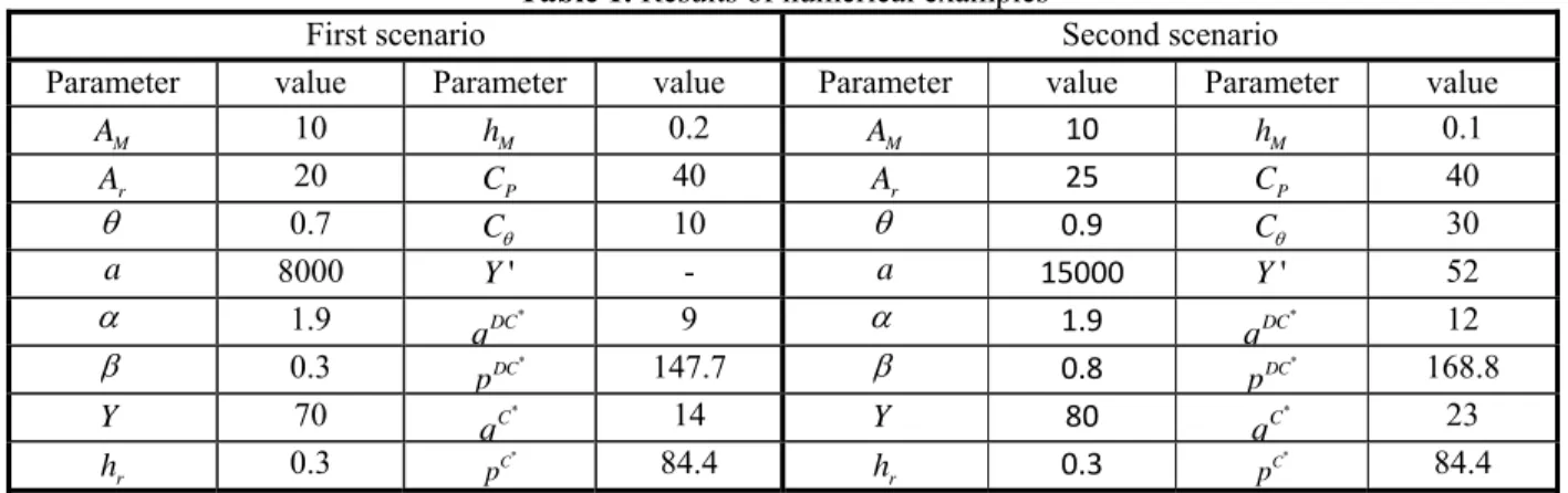
Table 1. Results of numerical examples

First scenario Second scenario

Parameter value Parameter value Parameter value Parameter value

M

A 10 hM 0.2 AM 10 hM 0.1

r

A 20 CP 40 Ar 25 CP 40

 0.7 C_ 10  0.9 C_ 30

a 8000 Y' - a 15000 Y' 52

 1.9 *

DC

q 9  1.9 DC*

q 12

 0.3 _DC*

p 147.7  0.8 _pDC* 168.8

Y 70 *

C

q 14 Y 80 C*

q 23

r

h 0.3 *

C

p 84.4 hr 0.3

*

C

p 84.4

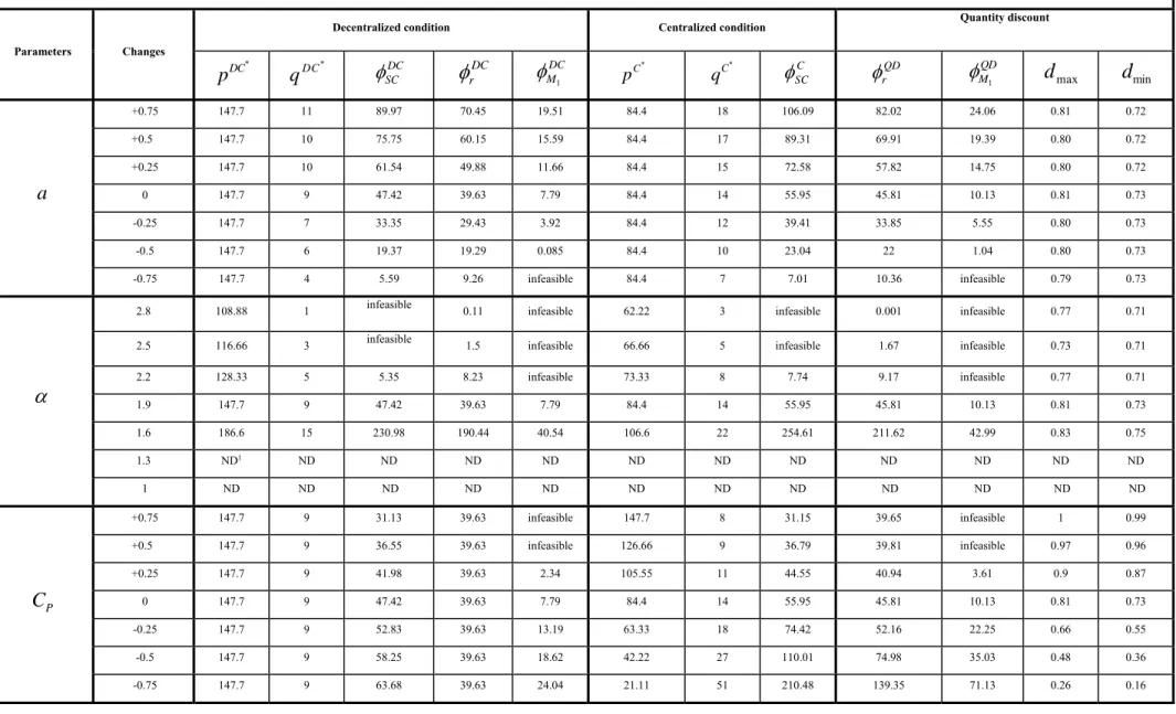
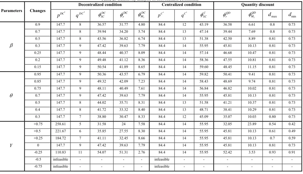
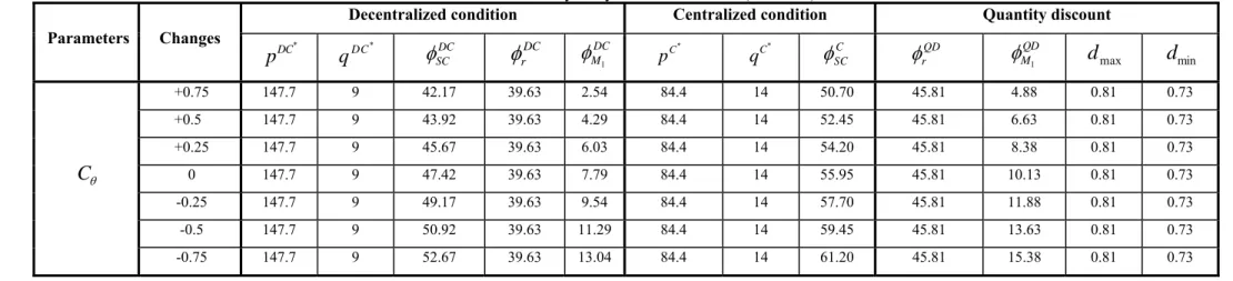
4-3- Sensitivity analysis

In this part we assess the effects of variations of some parameters on decision variables and profits. Therefore according to initial values of parameters and changing them, sensitive analysis is implemented. The results of these scenarios are illustrated in tables (2) and (3).

(13)

Table 2. Sensitivity analysis of first scenario

Parameters Changes

Decentralized condition Centralized condition Quantity discount *

DC

p

q

DC*



SCDC

DC r



DC₁ M



_C*

p

* C

q



SCC

QD r



1

QD M



d

max

d

min

a

+0.75 147.7 11 89.97 70.45 19.51 84.4 18 106.09 82.02 24.06 0.81 0.72

+0.5 147.7 10 75.75 60.15 15.59 84.4 17 89.31 69.91 19.39 0.80 0.72

+0.25 147.7 10 61.54 49.88 11.66 84.4 15 72.58 57.82 14.75 0.80 0.72

0 147.7 9 47.42 39.63 7.79 84.4 14 55.95 45.81 10.13 0.81 0.73

-0.25 147.7 7 33.35 29.43 3.92 84.4 12 39.41 33.85 5.55 0.80 0.73

-0.5 147.7 6 19.37 19.29 0.085 84.4 10 23.04 22 1.04 0.80 0.73

-0.75 147.7 4 5.59 9.26 infeasible 84.4 7 7.01 10.36 infeasible 0.79 0.73



2.8 108.88 1 infeasible 0.11 infeasible 62.22 3 infeasible 0.001 infeasible 0.77 0.71

2.5 116.66 3 infeasible 1.5 infeasible 66.66 5 infeasible 1.67 infeasible 0.73 0.71

2.2 128.33 5 5.35 8.23 infeasible 73.33 8 7.74 9.17 infeasible 0.77 0.71

1.9 147.7 9 47.42 39.63 7.79 84.4 14 55.95 45.81 10.13 0.81 0.73

1.6 186.6 15 230.98 190.44 40.54 106.6 22 254.61 211.62 42.99 0.83 0.75

1.3 ND1 _ND _ND _ND _ND _ND _ND _ND _ND _ND _ND _ND

1 ND ND ND ND ND ND ND ND ND ND ND ND

P

C

+0.75 147.7 9 31.13 39.63 infeasible 147.7 8 31.15 39.65 infeasible 1 0.99

+0.5 147.7 9 36.55 39.63 infeasible 126.66 9 36.79 39.81 infeasible 0.97 0.96

+0.25 147.7 9 41.98 39.63 2.34 105.55 11 44.55 40.94 3.61 0.9 0.87

0 147.7 9 47.42 39.63 7.79 84.4 14 55.95 45.81 10.13 0.81 0.73

-0.25 147.7 9 52.83 39.63 13.19 63.33 18 74.42 52.16 22.25 0.66 0.55

-0.5 147.7 9 58.25 39.63 18.62 42.22 27 110.01 74.98 35.03 0.48 0.36

-0.75 147.7 9 63.68 39.63 24.04 21.11 51 210.48 139.35 71.13 0.26 0.16

(14)

Table 2. Sensitivity analysis of first scenario (Continue)

Decentralized condition Centralized condition Quantity discount

*

DC

p

q

DC*



SCDC

DC r



DC₁ M



_C*

p qC*



SCC

QD r



1

QD M



d

_max

d

_min



0.9 147.7 8 36.57 31.77 4.80 84.4 12 43.19 36.58 6.61 0.8 0.73

0.7 147.7 8 39.94 34.20 5.74 84.4 13 47.14 39.44 7.69 0.8 0.73

0.5 147.7 8 43.56 36.82 6.74 84.4 13 51.38 42.50 8.89 0.81 0.73

0.3 147.7 9 47.42 39.63 7.79 84.4 14 55.95 45.81 10.13 0.81 0.73

0.25 147.7 9 48.44 40.37 8.09 84.4 14 57.14 46.68 10.47 0.81 0.73

0.2 147.7 9 49.48 41.12 8.36 84.4 14 58.36 47.55 10.81 0.81 0.73

0.15 147.7 9 50.54 41.89 8.65 84.4 14 59.60 48.45 11.15 0.81 0.73



0.95 147.7 9 50.36 43.57 6.79 84.4 14 59.82 50.41 9.41 0.81 0.73

0.85 147.7 9 49.32 42.09 7.23 84.4 14 58.43 48.69 9.74 0.81 0.73

0.75 147.7 9 48.11 40.49 7.61 84.4 14 56.84 46.82 10.02 0.81 0.73

0.7 147.7 9 47.42 39.63 7.79 84.4 14 55.95 45.81 10.13 0.81 0.73

0.5 147.7 8 44.02 35.71 8.31 84.4 13 51.58 41.21 10.37 0.81 0.73

0.4 147.7 8 41.72 33.32 8.40 84.4 13 48.71 38.41 10.29 0.81 0.73

0.3 147.7 7 38.80 30.47 8.33 84.4 12 45.09 35.07 10.03 0.80 0.73

Y

+0.75 258.61 5 31.58 24 7.58 84.4 14 55.95 32.05 23.89 0.54 0.42

+0.5 221.67 6 35.85 27.55 8.30 84.4 14 55.95 45.81 10.13 0.61 0.49

+0.25 184.72 7 41.11 32.45 8.66 84.4 14 55.95 45.81 10.13 0.7 0.59

0 147.7 9 47.42 39.63 7.79 84.4 14 55.95 45.81 10.13 0.81 0.73

-0.25 110.83 11 54.07 51.31 2.76 84.4 14 55.95 52.42 3.53 0.93 0.91

-0.5 infeasible - - - - infeasible - - - -

(15)

Table 2. Sensitivity analysis of first scenario (Continue)

Decentralized condition Centralized condition Quantity discount

*

DC

p

q

DC*



SCDC

DC r



DC₁ M



_C*

p qC*



SCC

QD r



1

QD M



d

_max

d

_min

C

_

+0.75 147.7 9 42.17 39.63 2.54 84.4 14 50.70 45.81 4.88 0.81 0.73

+0.5 147.7 9 43.92 39.63 4.29 84.4 14 52.45 45.81 6.63 0.81 0.73

+0.25 147.7 9 45.67 39.63 6.03 84.4 14 54.20 45.81 8.38 0.81 0.73

0 147.7 9 47.42 39.63 7.79 84.4 14 55.95 45.81 10.13 0.81 0.73

-0.25 147.7 9 49.17 39.63 9.54 84.4 14 57.70 45.81 11.88 0.81 0.73

-0.5 147.7 9 50.92 39.63 11.29 84.4 14 59.45 45.81 13.63 0.81 0.73

(16)

Decentralized condition Centralized condition Cost sharing contract

*

DC

p

q

DC*



SCDC

DC r



DC₁

M



_C*

p qC*



SCC

CS r



2

CS M





_max



_min

a

+0.75 168.8 15 148.85 120.98 27.88 84.4 30 195.19 - - infeasible infeasible

0 168.8 12 72.33 68.28 4.05 84.4 23 97.72 74.79 22.93 0.84 0

-0.25 168.8 10 46.94 50.81 infeasible 84.4 20 65.47 51.26 14.21 0.61 0

-0.5 168.8 8 21.68 33.42 infeasible 84.4 16 33.46 34.65 -1.20 0.396 0

-0.75 168.8 6 infeasible 16.20 infeasible 84.4 11 1.88 17.02 -15.14 0.19 0



2.8 124.44 2 Infeasible 0.298 infeasible 62.22 5 infeasible - - infeasible infeasible

2.5 133.33 3 infeasible 2.57 infeasible 66.67 8 infeasible 2.62 infeasible 0.022 0

2.2 146.67 6 infeasible 13.87 infeasible 73.33 14 3.68 15.08 infeasible 0.19 0

1.9 168.8 12 72.33 68.28 4.05 84.44 23 97.72 74.79 22.93 0.84 0

1.6 ND ND ND ND ND ND ND ND ND ND ND ND

1.3 ND ND ND ND ND ND ND ND ND ND ND ND

1 ND ND ND ND ND ND ND ND ND ND ND ND

P

C

+0.5 168.8 12 56.15 68.28 infeasible 126.67 16 59.72 - - infeasible infeasible

0 168.8 12 72.33 68.28 4.05 84.4 23 97.72 74.79 22.93 0.84 0

-0.25 168.8 12 80.37 68.28 12.09 63.33 30 134.41 - - infeasible infeasible

(17)

Table 3. Sensitivity analysis of second scenario (Continue)

Decentralized condition Centralized condition Cost sharing contract

*

DC

p

q

DC*



SCDC

DC r



DC₁ M



_C*

p qC*



SCC

CS r



2

CS M





_max



_min



0.95 168.8 12 70.70 67.18 3.52 84.4 23 95.68 73.35 22.35 0.83 0

0.9 168.8 12 71.23 67.55 3.69 84.4 23 96.37 73.85 22.53 0.83 0

0.85 168.8 12 71.76 67.91 3.85 84.4 23 97.05 74.34 22.71 0.84 0

0.8 168.8 12 72.33 68.28 4.05 84.4 23 97.72 74.79 22.93 0.84 0

0.6 168.8 12 74.46 69.77 4.69 84.4 23 100.48 76.85 23.63 0.86 0

0.4 168.8 12 76.68 71.30 5.38 84.4 23 103.29 78.90 24.39 0.88 0

0.2 168.8 12 78.94 72.85 6.08 84.4 24 106.17 81 25.17 0.9 0



- - - -

0.95 168.8 12 75.29 71.38 3.92 84.4 23 101.94 78.11 23.83 0.84 0

0.9 168.8 12 72.33 68.28 4.05 84.4 23 97.72 74.79 22.93 0.84 0

0.7 168.8 10 59.79 55.54 4.25 84.4 21 80.22 61.27 18.94 0.87 0

0.5 168.8 9 46.26 42.09 4.17 84.4 18 61.41 46.77 14.64 0.9 0

0.3 168.8 7 31.13 27.55 3.58 84.4 15 40.69 30.86 9.83 0.97 0

Y

0 168.8 12 72.33 68.28 4.05 84.4 23 97.72 74.79 22.93 0.84 0

-0.25 126.67 15 87.39 88.26 infeasible 84.4 23 97.73 88.61 9.12 0.1 0

-0.5 infeasible - - - - infeasible - - - -

(18)

Table 3. Sensitivity analysis of second scenario (Continue)

Decentralized condition Centralized condition Cost sharing

*

DC

p

q

DC*



SCDC

DC r



DC₁

M



_C*

p qC*



SCC

CS r



2

CS M





max



min

C

_

+0.75 168.8 12 52.07 68.27 infeasible 84.4 23 77.47 69.73 7.74 0.49 0

+0.5 168.8 12 58.82 68.27 infeasible 84.4 23 84.28 70.74 13.48 0.57 0

+0.25 168.8 12 65.58 68.27 infeasible 84.4 23 90.97 74.12 16.89 0.67 0

0 168.8 12 72.33 68.28 4.05 84.4 23 97.72 74.79 22.93 0.84 0

(19)

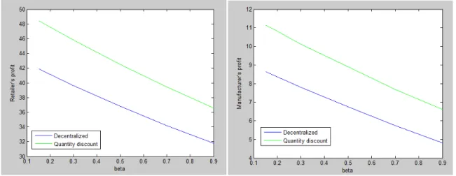
Fig 1. The effect of  on retailer’s profit (left) and manufacturer’s profit (right) under first scenario

According to demand function, green elasticity ( ) is exponent of greening level ( ) and it is a

number between zero and one. Therefore it is clear that increasing green elasticity induce to decrease demand. So by decreasing demand, member’s profit decrease too. Figure (1) indicates this fact clearly.

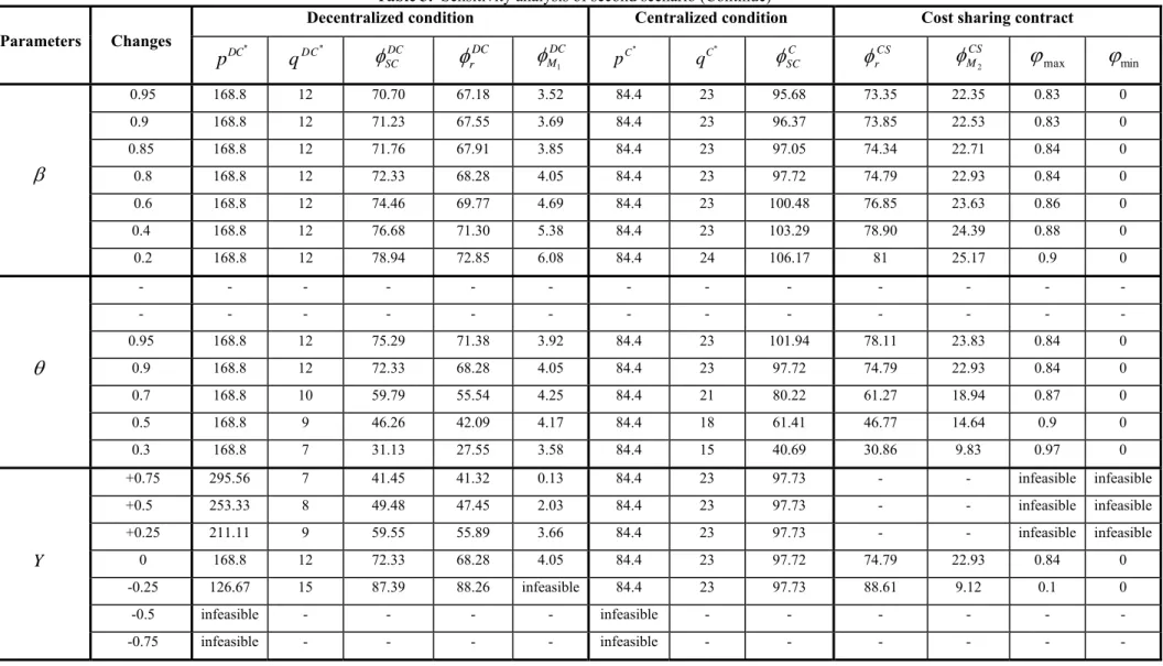
Fig. 2. The effect of  on retailer’s profit (left) and manufacturer’s profit (right) under first scenario

Considering the fact that higher greening level is so ideal for customers, retailer can sell more products

to them. As figure (2) represents, by increasing greening level, retailers’ profit is raised. In the other hand increasing greening level is so costly for manufacturer and it decreases the profit. This fact is obvious in this figure.

(20)

Fig 3. The effect of a on profit chain under first scenario (left) and second scenario (right)

Figure (3) Indicates that by increasing the market potential, profit chain for decentralized and centralized conditions increased under both scenarios. Actually by increasing market potential, the numbers of customers and also demand increase. So this fact causes to raise profit chain.

Fig 4. The effect of  on retailer’s profit (left) and manufacturer’s profit (right) under second scenario

Figure (4) represents the effect of  on members’ profit. Due to contrary relation between  and demand,

increasing the value of  causes to decrease demand and also members’ profit. As we mentioned customers

are looking for green products and it is clear that higher greening level of products attracts more customers attention. Therefore by increasing product greening level, the retailer buys more products from manufacturer and therefore sell more products to customers. So both members’ profits are increased by raising greening level of products. Additionally due to sharing greening costs, raising greening level has been beneficial for manufacturer and he/ she can achieve higher profit.

(21)

Fig 5. The effect of  on retailer’s profit (left) and on manufacturer’s profit (right) under second scenario

5- Conclusion

In this paper we considered a two-echelon green supply chain including two manufacturers and one

retailer and studied the effect of quantity discount and cost sharing contract on members profit. We calculated optimal values of decision variables under decentralized and centralized conditions and then we studied two scenarios. We intended to analyze the effect of designing contracts on profit. In first scenario quantity discount was offered to retailer by first manufacturer and in second scenario retailer proposed cost sharing contract to second manufacturer. Demand function was considered nonlinear and depends on price and product greening level. Although it was a function of greening level, we did not consider it as a decision variable. We reviewed the mathematical relations in both scenarios and in the following we assessed our proposed model by numerical example. After that sensitivity analysis is implemented to evaluate the effect of some parameters on decision variables and also profit.

As the results indicate, profit chain under centralized condition is higher than decentralized condition in both scenarios. Applying quantity discount and cost sharing contracts induced to make members’ profit higher than decentralized condition. Additionally the results shown that second manufacturer could achieve higher profit with respect to first manufacturer by cost sharing contract. Each of these contracts provides appropriate conditions for members of the chain to coordinate their business and increase the profit. Actually designing contracts is one of beneficial strategies for increasing profit. So managers and businessmen can employ different contracts to assist their organization to make higher profit. As future research authors can consider the following suggestions:

 Consider lead-time in your model

 Designing other contracts

(22)

References

Alfares, H.K., Ghaithan, A.M. (2016). Inventory and pricing model with price-dependent demand, time-varying holding cost, and quantity discounts, Computers& Industrial Engineering, 94: 170-177.

Alfares, H.k., Turnadi, R. (2016). General Model for Single-item Lot-sizing with Multiple Suppliers, Quantity Discounts, and Backordering , Procedia CIRP, 56: 199-202.

Avni, G., Tamir, T. (2016). Cost-sharing scheduling games on restricted unrelated machines, Theoretical Computer Science, 646: 26-39.

Basiri, Z., Heydari, J. (2017). A mathematical model for green supply chain coordination with substitutable products, Journal of Cleaner Production, 145: 232-249.

Bohner , Ch., Minner, S. (2016). Supplier Selection under Failure Risk, Quantity and Business Volume Discounts, Computers & Industrial Engineering, In press.

Burke, G.J., Geunes, J., Romeijn, H.E., Vakharia, A. (2008). Allocating procurement to capacitated suppliers with concave quantity discounts, Operations Research Letters, 36: 103-109.

Çebi, F., Otay, I. (2016). A two-stage fuzzy approach for supplier evaluation and order allocation problem with quantity discounts and lead time, Information Sciences, 339: 143-157.

Chalkley, M., Malcomson, J.M., (2002), Cost sharing in health service provision: an empirical assessment of cost savings, Journal of Public Economics, 84: 219–249.

Chao, G.H., Iravani, S.M.R., Savaskan, R.C. (2009). Quality Improvement Incentives and Product Recall Cost Sharing Contracts, MANAGEMENT SCIENCE, 55: 1122-1138.

Chang, Ch.T., Chiou, Ch.Ch., Yang, Y.W., Chang, Sh.Ch., Wang, W. (2010). A three-echelon supply chain coordination with quantity discounts for multiple items, International Journal of Systems Science, 41: 561-573.

Ghosh, D., Shah, J. (2015). Supply chain analysis under green sensitive consumer demand and cost sharing contract, International Journal of Production Economics, 164: 319-329.

Heydari, J., Govindan, K., Jafari, A. (2017). Reverse and closed loop supply chain coordination by considering government role, Transportation Research Part D: Transport and Environment, 52: 379-398. Hassanzadeh-Amin, S., Zhang, G., Akhtar, P. (2017). Effects of uncertainty on a tire closed-loop supply chain network, Expert Systems with Applications, 73: 82-91.

Chaharsooghi, S.K., Heydari, J., Nakhai Kamalabadi, I. (2011). Simultaneous coordination of order quantity and reorder point in a two-stage supply chain, Computers & Operations Research, 38(12), 1667-1677.

Heydari, J. (2014). Supply chain coordination using time-based temporary price discounts, Computers & Industrial Engineering, 75: 96-101.

(23)

Heydari, J., Norouzinasab, Y. (2015). A two-level discount model for coordinating a decentralized supply chain considering stochastic price-sensitive demand, Journal of Industrial Engineering International, 4(11): 531-542.

Heydari, J., Norouzinasab, Y. (2016). Coordination of Pricing, Ordering, and Lead time Decisions in a Manufacturing Supply Chain, Journal of Industrial and Systems Engineering, 9: 1-16.

Jackson, J.E., Munson, Ch.L. (2016). Shared resource capacity expansion decisions for multiple products with quantity discounts, European Journal of Operational Research, 253: 602-613.

Jiao, W., Zhang, J.L. (2017). The stochastic lot-sizing problem with quantity discounts, Computers & Operations Research, 80: 1-10.

Lau, A.H.L., Lau, H.Sh., Zhou, Y.W. (2008). Quantity discount and handling-charge reduction schemes for a manufacturer supplying numerous heterogeneous retailers, International Journal of Production Economics, 113: 425-445.

Leng, M., Parlar, M. (2010). Game-theoretic analyses of decentralized assembly supply chains: Non-cooperative equilibria vs. coordination with cost-sharing contracts, European Journal of Operational Research, 204: 96-104.

Lee, J.Y., Cho, R.K., Paik, S.K. (2016). Supply chain coordination in vendor-managed inventory systems with stockout-cost sharing under limited storage capacity, European Journal of Operational Research, 248: 95-106.

Mahdavi Mazdeh, M., Emadikhiav, M., Parsa, I. (2015). A heuristic to solve the dynamic lot sizing problem with supplier selection and quantity discounts, Computers & Industrial Engineering, 85: 33-43. Munson, C.L., Hu, J. (2010). Incorporating quantity discounts and their inventory impacts into the centralized purchasing decision, European Journal of Operational Research, 201: 581-592.

Nie, T., Due, Sh. (2017). Dual-fairness supply chain with quantity discount contracts, European Journal of Operational Research, 258: 491-500.

Ovaskainen, V., Hujala, T., Hänninen, H., Mikkola, J. (2017). Cost sharing for timber stand improvements: Inducement or crowding out of private investment?, Forest Policy and Economics, 74: 40-48.

Paratha Sarathi, G., Sarmah, S.P., Jenamani., M. (2014). An integrated revenue sharing and quantity discounts contract for coordinating a supply chain dealing with short life-cycle products, Applied Mathematical Modelling, 38: 4120-4136.

Paydar, M.M., Babaveisi, V., Safaei, A.S. (2017). An engine oil closed-loop supply chain design considering collection risk, Computers & Chemical Engineering, 104: 38–55.

Roma, P., Perrone, G. (2016). Cooperation among competitors: A comparison of cost-sharing mechanisms, International Journal of Production Economics, 180: 172-182.

Tamjidzad, Sh., Mirmohammadi, S.H. (2017). Optimal (r, Q) policy in a stochastic inventory system with