1144.pdf

ABSTRACT

James N. Struve. A Guidance Manual for the North Carolina

Pass/Fail Chronic Toxicity Test: Application to the OWASA

Mason Farm Wastewater Treatment Plant (Under the direction

of Dr. Philip C. Singer).

The objectives of this report are to provide the reader with

an understanding of the statistical tests utilized to interpret

chronic toxicity test data, and to examine the data to determine

problems associated with the test protocol. Chronic toxicity

data, obtained from the Orange County Water And Sewer Authority

(OWASA) Mason Farm Wastewater Treatment Plant (WWTP) in Carrboro,

NC, is analyzed to illustrate the underlying statistical concepts

and procedures, and to illustrate biomonitoring variability. A

spreadsheet was developed to compute the test statistics required

to compare mortality and reproduction data for an effluent sample

to those for a control sample, in accordance with the North

Carolina Division of Environmental Management requirements for

chronic toxicity tests. The spreadsheet was applied to two years

of chronic toxicity data from the OWASA Mason Farm WWTP.

A GUIDANCE MANUAL FOR THE

NORTH CAROLINA PASS/FAIL CHRONIC TOXICITY TEST:

APPLICATION TO THE OWASA MASON FARM WASTEWATER TREATMENT PLANT

TABLE OF CONTENTS

Page

List of Tables--- v

List of Figures--- vii

1. INTRODUCTION --- 1

1 .1 Format of the Report--- 2

2. BIOMONITORING --- 5

2.1 History--- 5

2.2 Acute vs Chronic Toxicity --- 10

2.3 North Carolina's Biomonitoring Program --- 14

2.4 Comparison of North Carolina's Biomonitoring

3. SOURCES OF WASTEWATER TOXICITY --- 24

3.1 Industrial Contributions --- 25

3.2 Chlorine--- 28

3.3 Ammonia--- 34

4. STATISTICAL METHODS--- 41

4.1 Introduction--- 41

4.2 Data Collection and Presentation---[—--- 42

4.3 Test for Normal Distribution of Data: Chi-Square Goodness of Fit Test--- 47

4.4 Test for Normal Distribution of Data:

Shapiro-Wi Ik's Test--- 50

4.5 Test for Homogeneity of Variance: Bartlett's Test--- 53

4.6 Parametric Test for Significant Difference in

Reproduction: Dunnett's Test Procedure --- 55

4.7 Non-Parametric Test for Significant Difference in Reproduction: Wilcoxon's Rank Sum Test --- 60

4.8 Test for Significant Difference in Mortality:

5. APPLICATION OF THE PASS/FAIL CHRONIC TOXICITY TEST AT THE OWASA MASON FARM WWTP--- 75

5.1 Wastewater Treatment Process --- 75

5.2 Influent/Effluent Quality --- 76

5.3 Chronic Toxicity Test Data--- 80

5.4 Statistical Analysis of Test Data--- 93

5.5 Correlation of Test Results with Effluent

Quality--- 99

TABLE OF CONTENTS (cent.)

Page

6. CONCLUSIONS---•--- 105

REFERENCES--- 107

Appendices A. Selected States' Biomonitoring Programs --- 112

B. Derivation and Calculation of Maximum Allowable ͣ Ammonia Concentrations Discharged to a Receiving Body of Water for Preservation of Aquatic Life --- 121

C. Statistical Tables Utilized to Interpret Chronic Toxicity Data--- 128

D. North Carolina Division of Environmental Management T Test--- 137

D.I Introduction--- 138

D.2 F Test--- 141

D.3 Equal Variance T Test--- 141

D.4 Unequal Variance T Test--- 143

D.5 Examples of T Test--- 144

E. Graphical Illustration of Monthly-Average Influent and Effluent Characteristics for OWASA Mason Farm WWTP--- 159

LIST OF TABLES

Page

Table 3.1: Priority Pollutants

Metals--- 26

GC/MS Acid Extractions--- 26

PCB/Pesticides --- 26

GC/MS Purgeables--- 27

GC/MS Base/Neutrual Extractables --- 27

Table 3.2: Residual Chlorine Levels Toxic to Aquatic Life--- 33

Table 3.3: Un-Ionized Ammonia Levels Toxic to Aquatic Life--- 39

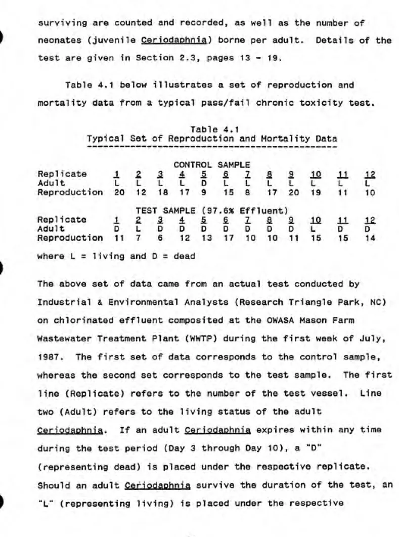
Table 4.1: Typical Set of Reproduction and Mortality Data--- 44

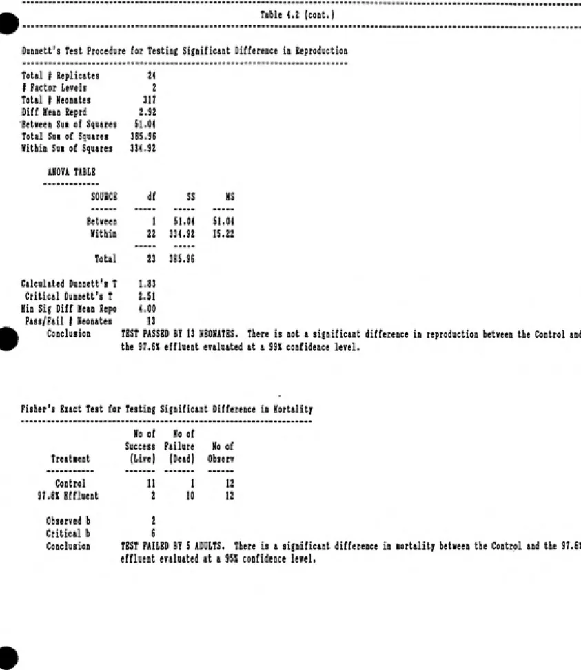
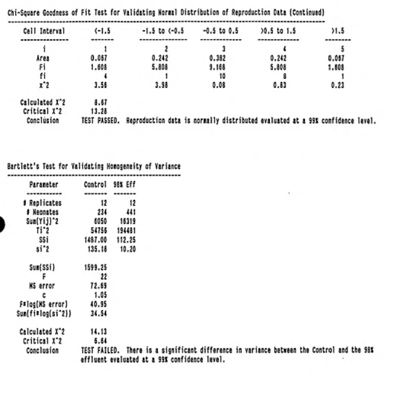
Table 4.2: OWASA #1 Statistical Spreadsheet Example Calculations --- 66

Table 4.3: OWASA #19 Statistical Spreadsheet Example Calculations --- 69

Table 4.4: OWASA #4 Statistical Spreadsheet Example Calculations --- 72

Table 5.1: Influent Wastewater Quality at the OWASA Mason Farm WWTP (Average Monthly Values) —- 77 Table 5.2: Effluent Wastewater Quality at the OWASA Mason Farm WWTP (Average Monthly Values) --- 78

Table 5.3: Selected OWASA Mason Farm WWTP Effluent Discharge Limits --- 79

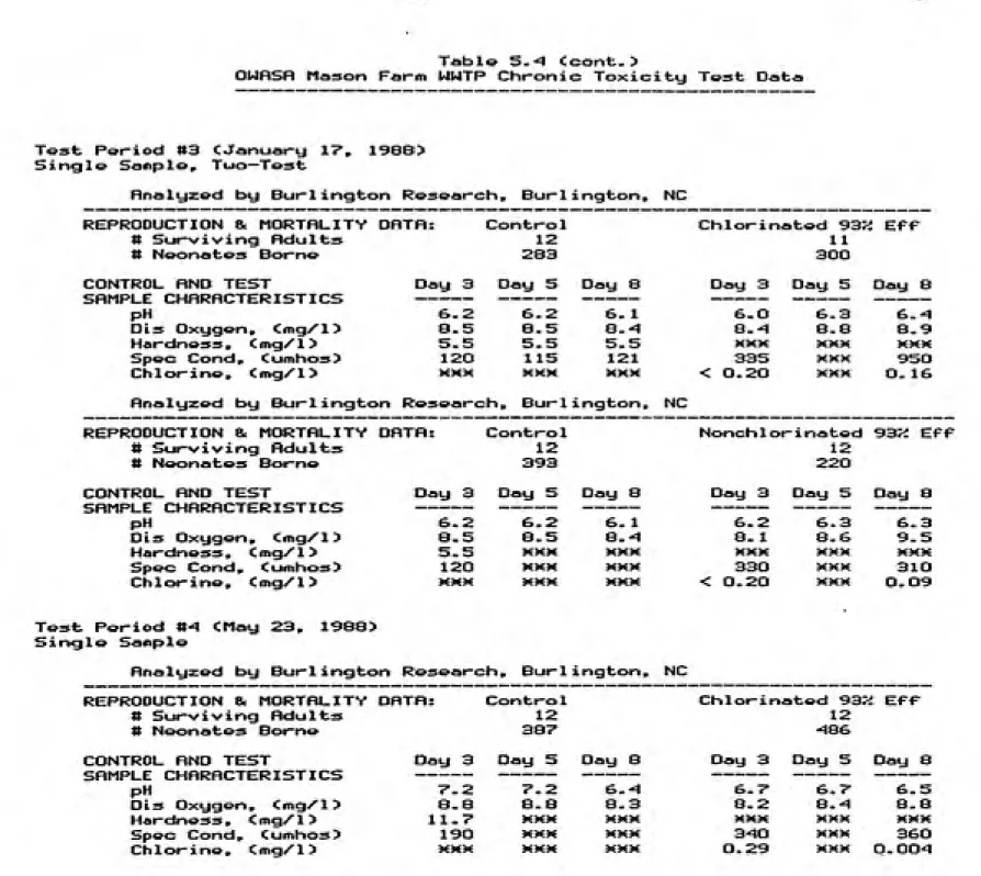
Table 5.4: OWASA Mason Farm WWTP Chronic Toxicity Test Data--- 81

Table 5.5: Ceriodaphnia Reproduction and Mortality Data (Chlorinated Samples from OWASA) --- 91

Table 5.6: OWASA Mason Farm WWTP Summary of Ceriodaphnia 7-Day Pass/Fail Chronic Toxicity Test Results--- 94

LIST OF TABLES (cont.)

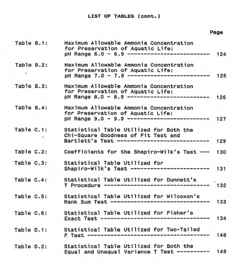
Page Table B.1: Maximum Allowable Ammonia Concentration

for Preservation of Aquatic Life:

pH Range 6.0 - 6.9--- 124

Table B.2: Maximum Allowable Ammonia Concentration for Preservation of Aquatic Life:

pH Range 7.0 - 7.9--- 125

Table B.3: Maximum Allowable Ammonia Concentration

for Preservation of Aquatic Life:

pH Range 8.0 - 8.9--- 126

Table B.4: Maximum Allowable Ammonia Concentration for Preservation of Aquatic Life:

pH Range 9.0 - 9.9--- 127

Table C.I: Statistical Table Utilized for Both the Chi-Square Goodness of Fit Test and

Bartlett's Test--- 129

Table C.2: Coefficients for the Shapiro-WiIk's Test --- 130

Shapi ro-Wi Ik's Test--- 131

Table C.4: Statistical Table Utilized for Dunnett's

T Procedure--- 132 Table C.5: Statistical Table Utilized for Wilcoxon's

Rank Sum Test--- 133

Table C.6: Statistical Table Utilized for Fisher's

Exact Test--- 134

Table D.I: Statistical Table Utilized for Two-Tailed

F Test--- 148

Table D.2: Statistical Table Utilized for Both the

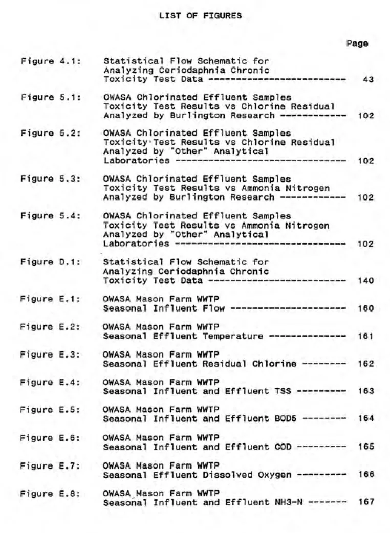
LIST OF FIGURES

Page

Figure 4.1: Statistical Flow Schematic for

Analyzing Ceriodaphnia Chronic

Toxicity Test Data--- 43

Figure 5.1: OWASA Chlorinated Effluent Samples

Toxicity Test Results vs Chlorine Residual

Analyzed by Burlington Research --- 102

Figure 5.2: OWASA Chlorinated Effluent Samples

Toxicity Test Results vs Chlorine Residual

Analyzed by "Other" Analytical

Laboratories --- 102

Figure 5.3: OWASA Chlorinated Effluent Samples

Toxicity Test Results vs Ammonia Nitrogen

Analyzed by Burlington Research --- 102

Figure 5.4: OWASA Chlorinated Effluent Samples

Toxicity Test Results vs Ammonia Nitrogen

Analyzed by "Other" Analytical

Laboratories --- 102

Figure D.I: Statistical Flow Schematic for

Analyzing Ceriodaphnia Chronic

Toxicity Test Data--- 140

Figure E.I: OWASA Mason Farm WWTP

Seasonal Influent Flow --- 160 Figure E.2: OWASA Mason Farm WWTP

Seasonal Effluent Temperature --- 161

Figure E.3: OWASA Mason Farm WWTP

Seasonal Effluent Residual Chlorine --- 162 Figure E.4: OWASA Mason Farm WWTP

Seasonal Influent and Effluent TSS —--- 163 Figure E.5: OWASA Mason Farm WWTP

Seasonal Influent and Effluent B0D5 --- 164 Figure E.6: OWASA Mason Farm WWTP

Seasonal Influent and Effluent COD --- 165

Figure E.7: OWASA Mason Farm WWTP

Seasonal Effluent Dissolved Oxygen --- 166

Figure E.8: OWASA Mason Farm WWTP

Seasonal Influent and Effluent NH3-N --- 167

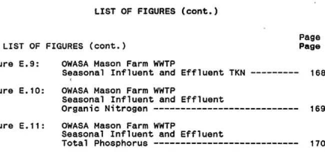
LIST OF FIGURES (cent.)

Page

LIST OF FIGURES (cont.) Page

Seasonal Influent and Effluent TKN --- 168 Figure E.10: OWASA Mason Farm WWTP

Seasonal Influent and Effluent

Organic Nitrogen --- 169

Figure E.11: OWASA Mason Farm WWTP

Seasonal Influent and Effluent

1. INTRODUCTION

A "whole effluent" chronic toxicity protocol was developed

by the United States Environmental Protection Agency (USEPA) as a

means to regulate surface water discharge of toxic substances.

This protocol was published in 1985 after five years of field and

laboratory investigations (USEPA, 1986). It contains discussions

on effluent sampling procedures, test organism culturing, chronic

testing methodology, and test data analysis. In essence, it is

to serve as a guidance manual for regulatory agencies as they

begin to establish water quality-based toxicity control programs.

The State of North Carolina was one of the first states to

implement whole effluent chronic toxicity testing by writing

toxicity requirements in their National Pollutant Discharge

Elimination System (NPDES) permits. North Carolina "extensively

reduced in complexity" USEPA's protocol "in order to provide a

relatively inexpensive means of assessing suitable water quality

with respect to chronically toxic substances" (North Carolina

Division of Environmental Management (NCDEM), 1988b). The major

difference between the two test protocols is in the number of

test concentrations and, consequently, the associated statistical

analysis procedures.

The protocol developed by the NCDEM determines the effects

of whole effluents on the mortality and reproduction of a species

for an extended period of time. Mortality and reproduction

results for the effluent sample are compared to those for a

control by performing statistical tests of significance.

However, after eighteen months of implementation, there still

appears to be confusion on how to statistically analyze the

chronic toxicity data. Furthermore, there is concern regarding

the validity and utility of the protocol due to conflicting test

results when split effluent samples are analyzed by independent

laboratories. There appears to be significant difficulties

associated with sample compositing and handling, culturing of the

test organism, and laboratory reproducibility of the test

protocol.

Therefore, the primary objectives of this report are to

provide the reader with an understanding of the statistical tests

utilized to interpret the chronic toxicity test data, and to

examine the data to determine problems associated with the test

protocol. Data obtained from the OWASA Mason Farm Wastewater

Treatment Plant in Carrboro, NC is analyzed to illustrate the

underlying statistical concepts and procedures, and to illustrate

1.1 Format of the Report

The succeeding chapters in this report are organized in the

Chapter 2 provides historical information regarding the

conception of biomonitoring, compares and contrasts acute

modifications in North Carolina's chronic toxicity protocol

relative to the USEPA's, and provides information regarding

biomonitoring programs in several other states. Chapter 3

discusses three of the principal sources of toxicity in municipal

wastewater. Concentrations toxic to aquatic organisms are

reported. Chapter 4 presents and explains the statistical

procedures employed to interpret chronic toxicity test data. In

addition, a statistical spreadsheet is introduced which

illustrates the necessary statistical computations. Chapter 5

describes the OWASA wastewater treatment processes as well as the

respective influent and effluent water quality characteristics.

OWASA chronic toxicity test data and results are presented and

re-analyzed making use of the spreadsheet developed.

Additionally, an attempt is made to relate toxicity test results

to effluent quality. Chapter 6 summarizes the conclusions of the

study.

Following Chapter 6 are six appendices. Appendix A provides

additional information regarding biomonitoring programs in the

other states surveyed. Appendix B presents a derivation and

calculation (based on pH and temperature) of the maximum allowable

ammonia concentration discharged to a receiving body of water for

preservation of aquatic life. Appendix C contains the

statistical tables utilized to interpret the chronic toxicity

data. Appendix D describes and illustrates the new statistical

procedure (T Test) that will be implemented after November 1,

1989 to analyze chronic reproduction data. Appendix E presents

the OWASA Mason Farm Wastewater Treatment Plant. Lastly,

Appendix F provides the statistical spreadsheets used to re¬

2. BIOMONITORING

2.1 History

The earliest use of aquatic invertebrates in tolerance

research was carried out to answer questions concerning adaption

and evolution over a century and a half ago. In the first

studies that were reported, freshwater invertebrates were

subjected to seawater, and marine invertebrates were exposed to

freshwater. Later, scientists conducted research on the effects

of ions in various combinations and concentrations on both

freshwater and marine invertebrates. It was only about five

decades ago that serious consideration was first given to the use

of aquatic invertebrates as test animals for the determination of

the toxicity of potential pollutants (Buikema and Cairns, 1980).

Almost all of the bioassay work that had been done prior to

the 1920's on the toxicity of various substances involved

concentrations that killed the test organism in a relatively

short time (an acute toxic response). The following

chronological list (Buikema and Cairns, 1980) recognizes the

founding fathers of biomonitoring who utilized aquatic

invertebrates as their test organism.

- The earliest report in which aquatic invertebrates were

involved in the basic aspects of bioassays appears to be

that of Beudant in 1816. Beudant conducted a series of

experiments in which he subjected 15 species of freshwater

- Bert in 1871 reported his observations on various

freshwater animals that he had immersed in seawater.

Among them were Daohnia.

- In 1925, Ramult set out to determine the concentrations of sodium chloride, Ringer's solution, and Van't Hoff's

solution that would restrain the development of pathogenetic eggs of Daphnia and other cladocerans.

- Strom in 1926 concerned himself with the effects of

altered hydrogen ion concentrations on Stentor. Diaptomus. and Daphnia.

- In 1928, Gresen published studies in which he attempted to

establish the highest salinities that five different genera would tolerate, the highest salinities that would

permit reproduction, and the highest salinities to which

these genera could become acclimated.

The use of Daphnia in bioassays really began with the work

of Naumann (Buikema and Cairns, 1980). In 1933 and 1934, Naumann

presented a series of 17 papers on the use of Daphnia magna as a

test animal, demonstrating that he could rear Daphnia magna

satisfactorily in water from many different sources (e.g., from soft humus waters to hard mineralized waters). Based on his observations, Naumann made the following recommendations with

respect to experimental animals (Buikema and Cairns, 1980):

1. Size class should be observed, since young animals often

have different sensitivities than older animals.

2. Changes from normal red color of animals should be noted,

since certain substances manifest their toxicity in a

color change.

3. Animals with large broods should be used, because some

toxic materials affect egg production.

4. Solutions should be maintained at the same constant

6. Tests should be carried out at a constant temperature of 20

degrees Celsius.

Naumann also found that certain conditions affect the

behavior of Daohnia magna (Buikema and Cairns, 1980):

1. Mechanical irritation causes animals to gather on the

bottom. .

2. Lack of oxygen causes animals to approach the surface.

3. Accumulation of animals at the side of vessels indicates unequal lighting.

4. Under conditions of irritation, Daohnia magna plunge more

or less senselessly through the medium, sometimes going

through "loopings". Normal swimming consists of hopping

movements - a rising with the sweep of the antennae

followed by a sinking.

In response to the environmental movement of the late 1960's

and early 1970's, the 92nd United States Congress passed the

Federal Water Pollution Control Act (FWPCA) Amendments (Public

Law 92-500) in 1972. One of the principal objectives of these

amendments was to restore and maintain the biological integrity

of the nation's waters and to achieve, by July 1, 1983, wherever

attainable, a quality of water that provides for the protection

and propagation of aquatic life. Recognizing the interdependence

of human health and welfare and aquatic life, Congress included

in this legislation the authorization and/or directives for the

United States Environmental Protection Agency (USEPA) and the

state environmental protection programs to conduct comprehensive

biological monitoring programs. Section 502 (15) of the FWPCA

defined biological monitoring as "the determination of the

(A) by techniques and procedures including sampling of organisms

representative of appropriate levels of the food chain

appropriate to the volume and the physical, chemical, and

biological characteristics of the effluent, and (B) at

appropriate frequencies and locations" (Worf, 1980). To achieve

the goals of this legislation, extensive effluent toxicity

screening programs were conducted during the mid 1970's by the

EPA regions and the states (Horning and Weber, 1985). ^

The setting of water quality-based contols for toxicity can

be accomplished in two ways. The first is the chemical specific

approach which involves setting limits for single chemicals based

on laboratory-derived no-effect levels for various test

organisms. The second is the "whole effluent" approach which

involves setting limits using effluent toxicity as a control

parameter. Traditionally, EPA has pursued the former approach to

regulate dischargers of toxic pollutants. Industrial dischargers

are required to analyze their wastewater for a number of widely

encountered toxic compounds (e.g., 126 Priority Pollutant List

and other "non-conventional" toxicants). However, it soon became

apparent that a chemical-specific approach, by itself, could not

adequately protect all surface waters because many toxic

compounds cannot be measured by available analytical methods.

Also, toxicological data are unavailable for the thousands of

potentially toxic compounds that are routinely discharged.

Additionally, toxicity data on the effects of individual

industrial and municipal wastewater. Recognizing this, EPA began

research on quick, reliable, and inexpensive biological testing

methods to measure the toxicity of complex effluents to a number

of vertebrate (Pimeohales oromelas. i.e. the fathead minnow),

invertebrate (Ceriodaohnia dubia). and plant species (Selenastrum

capricornutum) (Wall and Hammer, 1987).

In 1981, the EPA initiated the "Complex Effluent Toxicity

Testing Program." This program was initiated to support the

developing trend toward water quality-based toxicity control in

the National Pollution Discharge Elimination System (NPDES)

permit program. It was designed to investigate, under actual

discharge situations, the appropriateness and utility of "whole

effluent toxicity" testing in the identification, analysis, and

control of adverse water quality impacts caused by the discharge

of toxic effluents. The four objectives of the Complex Effluent

Testing Program are (USEPA, 1986):

1. To investigate the validity of effluent toxicity tests in

predicting adverse impact on receiving waters caused by

the discharge of toxic effluents.

2. To determine appropriate testing procedures which would

support regulatory agencies as they began to establish

water quality-based toxicity control programs.

3. To provide practical case examples of how such testing

procedures could be applied to effluents discharged to a

4. To field test short-term chronic toxicity tests involving

the test organisms, Ceriodaohnia and Pimeohales

prQmgla?-As part of the Complex Effluent Toxicity Testing Program,

industrial and municipal wastewater treatment plant (WWTP)

discharges at 8 sites across the country. In each case, toxicity

testing identified those effluents which were toxic, and

predicted whether the effluent was causing toxic effects in the

receiving water. Effects on the receiving water were confirmed

by biosurvey data (Wall and Hammer, 1987).

On March 9, 1984, the USEPA issued a national policy

statement recommending that state and regulatory agencies use

biological techniques as a complement to chemical-specific

analyses when assessing effluent discharge toxicity, and that

they use effluent toxicity as a control parameter in writing

permit limits (Wall and Hammer, 1987). Thus, NPDES permit limits

are written based not only on national guidelines, but also on

site-specific water quality considerations.

2.2 Acute vs Chronic Toxicity

Toxicity refers to the potential for a substance to have an

adverse or harmful effect on a living organism. A toxicant is an

agent (e.g., a specific chemical or a chemical mixture such as

effluent wastewater) that can produce an adverse effect in a

biological system, seriously damaging its structure or function

or producing death. The adverse effects can either be

categorized as acute or chronic. Acute effects are those that

occur rapidly as a result of short-term exposure to a high

concentration of the toxicant. Acute effects are relatively

severe and are characterized by lethality of the test organism.

produces deleterious effects due to repeated or long-term

exposures to a relatively low concentration of the toxicant.

There may be a relatively long latency period for the expression

of these effects, particularly if the exposure concentration is

very low. Chronic effects are sublethal and may include:

behavioral changes (alteration of swimming, attraction-avoidance,

and prey-predator relationships), physiological changes (growth,

reproduction, and development), biochemical changes (blood enzyme

and ion levels), and histological changes. Thus, toxicity tests

were developed to evaluate the concentration of the toxicant and

the duration of exposure required to produce such adverse effects

on a living test organism under standardized, reproducible

conditions (Rand and Petrocelli, 1985).

During a chronic toxicity test, aquatic organisms are

exposed to the toxicant continuously during an entire

reproductive life cycle to evaluate the toxicant's effect on

reproduction and growth. Generally, the concentration of

toxicant that produces chronic effects is lower than that which

produces the more-readily observable acute effects such as

mortality. Therefore, chronic toxicity tests can provide a more

sensitive measure of toxicity than acute toxicity tests (Rand and

Petrocelli, 1985). For this reason, regulatory agencies often

require (as written in the discharger's permit) the use of a

seven-day (chronic), static renewal, toxicity test which uses the

cladoceran, Ceriodaohnia dubi^. as the aquatic test organism for

freshwater discharges. Static refers to batch exposure in

contrast to continuous exposure as in a flowing system.

Therefore, a static renewal test is one in which the test

solutions and control water are renewed periodically by

transferring the test organisms to chambers with freshly-prepared

test solutions. This test is initiated with neonates (juvenile

Ceriodaphnia) less than 24-hours old and within 4-hours of age of

each other (NCDEM, 1988b).

The static renewal test method is preferred over the static

non-renewal test (in which the test organism is exposed to the

same effluent concentration throughout the duration of the test)

because of toxicant adsorption on the walls of the test chamber,

uptake of the toxicant by the test organism, bi©degradation of

the toxicant by microorganisms, and the effect of metabolites on

toxicity (Peltier and Weber, 1985). It is also preferred over

the flow-through test (in which the test organism is exposed to a

continuous flow of "fresh" effluent during the entire test

period) for the following reasons (Peltier and Weber, 1985):

1. It is simple and inexpensive.

2. It is cost-effective.

3. Limited resources are required (e.g., manpower, space,

and equipment). Therefore, staff can perform many

sequential tests on samples over time.

4. It requires a small volume of effluent sample

(approximately 1 to 20 liters).

5. It provides some indication of toxicity persistence.

1. It does not reflect temporal changes in effluent

composition and toxicity.

2. There may be a dissolved oxygen (DO) demand exerted by

the waste, leading to DO depletion.

3. Toxicants can be lost due to volatilization, adsorption

to the test vessel, or biodegradation.

Cladocerans, also known as "water fleas", have been used in

tolerance studies for over a century (Standard Methods, 1985).

There are several reasons why cladoceran species (e.g., Daohnia

magna. Daohnia oulex. Ceriodaohnia reticulata. Ceriodaohnia

dubia) have been extensively used as test organisms for aquatic

toxicity testing. First, they are macroscopic and do not require

the use of a microscope. However, they are smaller than most

fish and, hence, require less space and less toxicant for

purposes of testing. Because of the difference in space,

equipment, and toxicant requirements, the cost of equipping and

running an aquatic invertebrate toxicity laboratory is

approximately one-tenth the cost of equipping and running a

similar fish toxicity laboratory (Buikema and Cairns, 1980).

Second, reproduction and life-cycle studies may often be

completed within 2 to 4 weeks utilizing cladocerans as test

organisms, whereas life-cycle studies with rapidly-reproducing

fish (e.g., flagfish and zebra fish) may require as long as 3

months. Hence, the use of cladocerans can result in more

toxicants and/or more species being tested within a given time

than would be possible if fish alone were used (Buikema and

Cairns, 1980). Third, Mount and Norberg (1984) have found

cladocerans to be readily available, adaptable to laboratory

conditions, and one of the more sensitive aquatic animals to test

chemicals. They also state that "the functional role of

cladocerans in the community is less often mentioned as a reason

for using them as test animals." They go on to say that

cladocerans "are among the most important groups converting

phytoplankton and, perhaps more importantly, bacteria into animal

protein that is nutritionally valuable for higher animals, such

as fishes. Thus, their important role in aquatic communities

makes them logical choices for inclusion among species that need

to be protected."

Ceriodaohnia dubia has been found to be the best cladoceran

choice as a test animal due to their ease of culturing in the

laboratory, their young (neonates) are easier to count, the

adults produce large broods, and ephippia (a protected dormant

stage of the daphnid life cycle which indicates unfavorable

conditions and an unhealthy population) are uncommon even in

crowded cutures (Mount and Norberg, 1984). As far as sensitivity

to toxicants is concerned. Mount and Norberg compared the 48-hour

LC50 (LC50 is defined as the concentration estimated to cause

mortality in 50% of the test population over a specified time

period) data for four cladoceran species (Q^ magna. D. pulex. C.

reticulata, and Sj. vetulus) to 13 toxic substances. The data

suggest that none of the four species were distinctly more

sensitive than any of the others.

2.3 North Carolina's Biomonitoring Program

either an acute or a chronic response. Consequently, both acute

and chronic tests have been developed to evaluate the adverse

effects of a toxicant. Presently, in the State of North

Carolina, most dischargers are required to monitor for chronic

effects and not acute effects. However, in instances where the

receiving stream or mixing zone is almost entirely effluent.

North Carolina's Division of Environmental Management (NCDEM)

often requires the use of an acute methodology in which acute

mortality in a specific effluent can be statistically determined

(NCDEM, 1988b).

NCDEM has modified EPA's standard acute method (Methods for

Measuring %hs. Acute Toxicity q± EfflM^ntg %Q. Freshwater snd

Marine Organisms. EPA/600/4-85/013) in order to test higher

effluent concentrations where a measured LC50 may not necessarily

protect for acute toxicity. NCDEM's acute testing procedure is

outlined in its July 1988 information packet entitled "AQUATIC

TOXICITY TESTING - Understanding and Implementing Your Testing

Requirement" and is summarized as follows:

The acute procedure is a static non-renewal toxicity

test using either the Pimeohales promelas (fathead minnow), Dj.

Pulex. or Qj_ dubia. Two sample populations are utilized in this

procedure with the control population specified as sample "one"

and the effluent specified as sample "two". Generally, the

effluent concentration is diluted to 90%; however, the actual

concentration is specified either in the NPDES permit or by the

NCDEM. Each sample is tested using four identical test vessels

each containing ten test organisms. At the end of the test

period (48-hours), all organisms are identified as alive or dead.

The data are then statistically analyzed by using a Standard Student T Test to determine if mortality in the effluent is

significantly different than the control population evaluated at

a 99X confidence level.

In contrast to NCDEM's acute toxicity test, the North Carolina Pass/Fail Chronic Toxicity Test measures both Ceriodaohnia survival and reproduction during a 7-day test period. The test is performed on two samples. Twelve female adult Ceriodaohnia are exposed to each sample in individual test chambers containing 15 mL of solution. The first sample is

considered as the control population and is dosed at 0% effluent

and 100% culture water. Culture water is defined as the same

source of water as that used to maintain the test organism

population in the laboratory. This sample serves as a control to evaluate the significance of the response in sample two. Sample two exposes the test organisms to the predicted instream waste concentration of the effluent. The instream waste concentration of the effluent is obtained by diluting the effluent with culture

water as follows:

Percent (Permitted Discharge Volume)*(100)

Instream =

---Waste Cone (Permitted Discharge Volume + 7Q10) where 7Q10 is the lowest average 7-day flow in the

receiving stream which has a probability of recurrence

every ten years.

concentration equivalent to instream low flow values, has

significant detrimental impact upon reproduction as compared to

the control population. If there is no significant detrimental

impact compared to the control population, then the effluent

discharged to the receiving stream is not considered chronically

toxic to instream organisms/populations, and is considered to

have passed the toxicity test. However, if there are significant

differences in either reproduction or mortality between the test

and the control samples, then the effluent disharged to the

receiving stream is considered chronically toxic, and is

considered to have failed the test (NCDEM, 1988b).

The day to day procedures of the North Carolina Pass/Fail

Chronic Toxicity Test are briefly summarized as follows (NCDEM,

1988b).

Day 1: Discharger begins compositing 24-hour effluent sample. Composited sample should be refrigerated or cooled by ice to maintain a temperature less

than or equal to 4 deg C. A minimum effluent sample volume of 500 mL is collected.

Day 2: Discharger collects, packages, and ships 24-hour composite sample to analyzing laboratory where

toxicity test is performed. Care should be taken to ensure effluent sample temperature upon

arrival at laboratory is less than or equal to 4

deg C.

Day 3: The toxicity test is initiated as the test

organisms (Ceriodaphnia) are introduced to the

control and test samples. Dissolved oxygen, temperature, pH, and specific conductance are measured and recorded in both the control and

test samples. In addition, chlorine residual

is measured and recorded in the test sample;

hardness is measured and recorded for the control

sample. Dissolved oxygen should be greater than or equal to 5.0 mg/1 and the temperature maintained

at 25 deg C (+ or - 1 deg C). The Ceriodaphnia are

fed.

Day 4: Discharger begins compositing second 24-hour effluent composite sample. Ceriodaphnia in the test solutions are fed.

Day 5: Ceriodaphnia are transferred to new solutions of

the original composite test sample and control sample. Mortality and reproduction counts are performed at this time. Also, dissolved oxygen, temperature, and pH are measured and recorded for both the original composite test and control

samples. Discharger collects, packages, and ships second 24-hour composite sample to laboratory. Ceriodaphnia are fed.

Day 6: Laboratory refrigerates and maintains second composite effluent sample's temperature at less than or equal to 4 deg C. Ceriodaphnia are fed.

Day 7: Same as Day 6.

Day 8: Renew all test solutions by transferring the

respective organisms to either the second composite test sample or to the new control sample.

Mortality and reproduction counts are performed. Dissolved oxygen, temperature, and pH are measured

and recorded in both the discarded and the new

second sample for both the composite test and control samples. In addition, specific conductance and

chlorine residual are measured and recorded in the

second composite test sample. Specific

conductance and hardness are measured and recorded

in the new control sample. Ceriodaphnia are fed. Day 9: Ceriodaphnia are fed.

Day 10: Perform final mortality and reproduction counts as well as measure and record dissolved oxygen,

temperature, and pH. Begin statistical analysis to determine if there is a significant difference

in either mortality or reproduction between the

control and the test samples.

The North Carolina Pass/Fail Chronic Toxicity Test is a modified version of the USEPA's protocol entitled Methods for Estimating %hs. Chronic Toxicity af Effluents and Receiving Viaisrs

to Freshwater Organisms. EPA-600/4-85-014. The reasoning behind

means of assessing suitable water quality with respect to

chronically toxic substances" (NCDEM, 1988b).

The major difference between the two test protocols is in

the number of test concentrations and, consequently, the

associated statistical analysis procedures. NCDEM's protocol

yields data that either accepts or rejects an effluent for

discharge to a specific body of water. It does not determine the

"no observable effect concentration" (NOEC), i.e. the safe

concentration below which no impact is expected to occur. At

times, however, it may be necessary to determine the NOEC in

order to evaluate the degree of toxicity reduction needed. In

that instance, EPA's methodology of using an expanded series of

dilutions is employed.

The USEPA's protocol suggests exposing the test organism to

five test concentrations and a control. This contrasts with

NCDEM's pass/fail test which uses only one test concentration and

a control. The test concentrations in the USEPA's dilution

series is established around the instream waste concentration by

factors of three. The highest concentration is two multiples

above the instream waste concentration and the lowest is two

multiples below that concentration. For example, if the low flow

instream waste concentration is 5%, then the exposure

Concentration % Multiple 45 15 X 3

15 IWC X 3 5 0

1.5 IWC / 3 0.45 1.5/3

Control Not Applicable

where IWC is the instream waste concentration

The chronic value, also called the "maximum acceptable

toxicant concentration" (MATC) is calculated as the geometric

mean of the lowest observable effect concentration (LOEC) and the

NOEC. This hypothetical concentration is in a range bounded at

the lower end by the highest concentration in the chronic test

that produces no effect (NOEC), and at the higher end by the

lowest concentration tested that produces a statistically

significant effect (LOEC) (Rand and Petrocelli, 1985). If the

chronic value lies above the range of concentrations, then the

effluent is of minimal concern regarding toxics tested in the

discharge. However, should the lowest concentration be impacted

in comparison to the control, then the toxicity of the effluent

must be viewed as harmful to the receiving stream and will not

meet the pass/fail criteria (the pass/fail criteria and the

underlying statistics are discussed in Chapter 4).

Due to NCDEM's smaller sample size (one test concentration

as compared to the USEPA's five), NCDEM requires a greater

confidence level, i.e. more proof, in order for a discharger to

fail a test than does the USEPA. Consequently, NCDEM requires

reproduction data to be evaluated at a 99X confidence level,

2.4 Comparison of North Carolina's Biomonitoring Program with

Selected Other States

One of the first states to recognize the adverse effects of biocides (chemicals used to kill bacteria and other

microorganisms) in wastewater discharges, North Carolina emerged as a national leader in using aquatic toxicology as a regulatory tool. But how does North Carolina's program compare to programs in other states? To try to answer this question, the author intended to contact and survey selected states within several of EPA's 10 regions regarding their biomonitoring programs. This plan of attack was quickly abandoned after contacting the states within EPA Region 1 and not obtaining much useful information.

It appears that most of the states in EPA Region 1

(Massachusetts, New Hampshire, Maine, Rhode Island, Vermont, and Connecticut) are only requiring acute toxicity testing of

industrial process discharges at this time, and requiring

municipal wastewater treatment plants only to monitor the chronic toxicity of their final effluent in order to establish a data base. In addition, three of the states (Vermont, Rhode Island, and Connecticut) have dechlorination policies or foresee adopting dechlorination policies in the near future.

It appears that the State of Connecticut has the most developed program of the six states surveyed. That state has written acute toxicity limits into their industrial NPDES

permits; these limits are enforceable. Connecticut follows EPA's standard acute protocol, but utilizes application factors for establishing toxicity limits (e.g., 3 for acute and 20 for

chronic, corresponding to limits of LC50/3 and LC50/20,

respectively). In addition, since May of 1988, all industries must submit a "Discharge Toxicity Evaluation." This report states the type of waste being discharged, how it is being treated, and the type of monitoring program being employed. Connecticut also requires municipal WWTPs to monitor for acute toxicity, but their permits do not contain limits. The state has modified EPA's acute pass/fail test for municipal dischargers and dischargers who discharge in low flow streams (i.e., minimal

dilution effect). The modified version is referred to as the "No Kill Protocol." This method calls for 5 effluent test

populations and 3 control populations. The mean survival for both the 5 test samples and 3 controls must be 90X in order to constitute a passing result.

In summary, most of the states in EPA Region 1 are just beginning to implement their biological monitoring programs, and consequently, their data bases are relatively scarce. For

further information regarding their respective biomonitoring programs, refer to Appendix A.

Even though the State of Colorado was not contacted, their unique approach towards biomonitoring deserves discussion.

Colorado has received considerable attention regarding their biomonitoring program due to their recent articles published in the Journal of the Water Pollution Control Federation (Grimes, 1987; Michael, Egan, and Grimes, 1989). Colorado has based

contrast to North Carolina's strict liability approach. To

clarify this point, enforcement action is based not on the

results of individual biomonitoring tests, but on the diligence

with which dischargers detect and pursue elimination of toxicity

in their final effluent (Michael, Egan, and Grimes, 1989). The

major features of Colorado's biomonitoring regulations (Michael,

Egan, and Grimes, 1989) are summarized below:

1. NPDES permit limits are established only for acute

toxicity. However, chronic toxicity testing is required

of effluents discharged to aquatic-sensitive streams as

an information gathering tool only. This is due to the

fact that no Toxicity Reduction Evaluation (TRE) procedures relevant to chronic toxicity have been

developed.

2. Enforcement is based on the discharger displaying a lack

of diligence (defined in terms of the timely performance of specified requirements at an acceptable level of

effort). The diligence approach recognizes the

fundamental differences between conventional pollutants and toxics. Publicly owned treatment works (POTWs) are only held accountable for those process elements within

their control. Another item of importance to POTWs is

that the regulation recognizes the possibility that existing technology may not be able to identify causes,

sources, or treatment options for toxicity in complex POTW effluents.

3. Toxicity incidents are defined by detecting a pattern of

toxicity rather than by a single biomonitoring test

result. Thus, POTWs are not held responsible for

isolated events such as spills or "midnight dumps" into

their collection system.

4. All investigations and control program requirements are designed under the oversight and approval of the

permitting authority. The permitting authority becomes

a knowledgeable and active partner in the process of

toxicity control rather than a mere enforcement agency.

3. SOURCES OF WASTEWATER TOXICITY

If a pattern of whole effluent toxicity has been established in a discharger's final effluent, the next steps are to first identify the toxicant(s), and then to remove the causative

agent(s) or to eliminate the contributing factors. As a result, the USEPA Environmental Research Laboratory in Duluth, Minnesota has published a series of guidance documents intended to aid the discharger in conducting aquatic Toxicity Identification

Evaluations (TIEs) as part of an overall Toxicity Reduction Evaluation (TRE). EPA's approach is divided into three phases: Phase I contains methods to identify the physical/chemical nature of the constituent(s) causing toxicity without specifically

identifying the toxicant(s); Phase II describes methods to specifically identify the toxicant(s) if they are non-polar organics, ammonia, or metals; and Phase III desribes methods to confirm the suspected toxicant(s) (Mount and Anderson-Carnahan,

1988).

Once the toxicant has been identified, bench- or pilot-scale treatability studies can be performed to examine options for

removing the toxicant(s). Possible treatment processes include coarse and/or fine media filtration, chemical reduction by

wastewater system can be pursued.

Possible sources of municipal whole effluent toxicity (e.g., industrial contributions, residual chlorine and chlorination by¬ products due to disinfection practices, and ammonia) are

discussed below.

3.1 Industrial Contributions

Traditionally, most wastewater treatment plants were designed to remove suspended solids and biodegradable organic material (i.e., BOD). Nutrient removal (nitrogen and phosphorus) was introduced in the late 1960's and early 1970's. During this same time frame, America was experiencing a chemical revolution as new synthetic chemicals were developed for a myriad of uses (e.g., the application of herbicides and pesticides to increase agricultural production, and the utilization of lubricants and solvents to enhance industrial operation). As man's technology advanced and his dependence on synthetic chemicals continued, chemical compounds in concentrations deleterious to aquatic life

were detected in final wastewater effluents. The sources of

these harmful chemicals are attributed principally to industrial wastes, but they may also be derived from surface runoff (both urban and rural) and domestic discharges. Due to the presence of these harmful chemical compounds in municipal wastewaters,

regulatory agencies have begun to write "priority pollutant" limits into NPDES permits. Currently, 126 chemicals constitute the priority pollutants. These 126 priority pollutants are

further subdivided as either metals (14), GC/MS acid extractables

(11), PCB/pesticides (27), GC/MS Purgeables (31), or

GC/MS/neutral extractables (43). Table 3.1 below lists the 126 priority pollutants.

Table 3.1

Priority Pollutants Metals

Compound

Cyanide

SiIver Arsenic

Beryl 1ium Cadmium

Total Chromium

Copper

Compound

Mercury Nickel

Lead

Antimont Selenium

Zinc

Thai 1ium

GC/MS Acid Extractables

Compound Compound

4-Chloro-3-Methylphenol 2-Chlorophenol

2,4-Dichlorophenol 2,4-Dimethylphenol 2,4-Dinitrophenol

2-Methyl-4,6-Dinitrophenol

2-Nitrophenol 4-Nitrophenol Pentachlorophnol

Phenol

2,4,6-Trichlorophenol

PCB/Pesticides

Compound Compound

alpha-BHC 4,4'-DDT

beta-BHC Endrin Ketone

delta-BHC Methoxychlor

gamma-BHC (Lindane) alpha-Chlordane

Heptachlor gamma-Chlordane

Aldrin _Toxaphene

Heptachlor Epoxide PCB 1016

Endosulfan I PCB 1221

Dieldrin PCB 1232

4,4'-DDE PCB 1242

Endrin PCB 1248

Endosulfan II PCB 1254

4,4'-DDD PCB 1260

Table 3.1 Priority (Continued) Pollutants GC/MS Purgeables Compound Benzene

Bromod i ch1oromethane Bromoform Bromomethane Carbon Tetrachloride Chlorobenzene Chloroethane 2-Chloroethylvinyl Ether Chloroform Chioromethane Di bromochloromethane 1,2-Dichlorobenzene 1,3-Dichlorobenzene 1,4-Dichlorobenzene 1,1-Dichloroethane Compound trans-1,2-Dichloroethene 1,2-Dichloropropane cis-1,3-Dichloropropene trans-1,3-Dichloropropene Ethyl Benzene Methylene Chloride 1,1,2,2-Tetrachloroethane Tetrachloroethene Toluene 1,1,1-Trichloroethane 1,1,2-Trichloroethane Trichloroethene Trichlorofluoromethane Vinyl Chloride

GC/MS Base/Neutral Extractables

Compound

Acenaphthene Acenaphthylene Anthracene

Benzo (a) Anthracene

Benzo (a) Pyrene

Benzo (b) Fluoranthene

Benzo (ghi) Perylene

Benzo (k) Fluoranthene

Bis (2-Chloroethoxy) Methane Bis (2-Chloroethyl) Ether Bis (2-Chloroisopropyl) Ether Bis (2-Ethylhexyl) Phthalate

4-Bromophenyl Phenyl Ether Benzyl Butyl Phthalate 2-Chloronaphthal6ne

4-Chlorophenyl Phenyl Ether Chrysene

Dibenzo (a,h) Anthracene 1,2-Dichlorobenzene 1,3-Dichlorobenzene 1,4-Dichlorobenzene 3,3'-Dichlorobenzidine Compound Diethyl Phthalate Dimethyl Phthalate Di-N-Butyl Phthalate

2,4-D i n i troto1uene

2,6-Dinitrololuene Di-N-Octy1phthalate

Fluoranthene Fluorene

Hexachlorobenzene

Hexach1orobutad i ene

Hexachlorocyclopentadiene

Hexachloroethane

Indeno (1,2,3-cd) Pyrene

Isophorone Naphthalene Nitrobenzene

N-Nitrosodipropyl amine N-N i trosod i pheny1 am i ne

Phenanthrene Pyrene

1,2,4-Trichlorobenzene

Of the 126 priority pollutants, metals (e.g. cadmium, nickel, chromium, lead, copper and zinc) are associated

principally with metal plating industries; phenols, solvents (e.g. carbon tetrachloride), and solvent weld by-products (e.g. trichloroethene and tetrachloroethene) are characteristically found in industrial wastewaters; and pesticides (e.g. endosulfan, 4,4'-DDT and aldrin) are attributed to surface runoff from

agricultural farmland.

Influent wastewater to OWASA's Mason Farm WWTP is

principally domestic in origin with appreciable amounts of urban storm water runoff. Except for the University of North Carolina at Chapel Hill, there are no industrial contributors. Therefore, the remainder of this discussion focuses on the two other key potential toxics, chlorine and ammonia.

3.2 Chlorine

- Wastewater Chlorination

Over the past century, chlorination has evolved as the most commonly used method of disinfecting both water and wastewater.

The extensive use of chlorine has come about as a result of its

bactericidal effectiveness, ease of application, relatively low cost, and relatively persistent residual (Aieta, 1980). It has not been until the past decade, however, that its possible

detrimental effects have been considered. Two of the most

for these and other reasons that the indiscriminate practice of

wastewater chlorination for the purpose of disinfection is

presently undergoing review in the United States.

Prior to the 1970's, regulations governing wastewater

disinfection were at the discretion of the individual states.

Some states required either year-round disinfection or no

disinfection at all, whereas other states allowed either seasonal

disinfection or mandated disinfection on a case-by-case basis.

The implementation of mandatory effluent disinfection

drastically changed in August 1973 when the Federal Government,

through the USEPA, assumed regulatory control with the passage of

Public Law 92-500, the Federal Water Pollution Control Act

(FWPCA). The vast majority of wastewater treatment plants could

not meet the imposed maximum concentration of 2000 fecal

coliforms per 100 mL and were thus forced to employ a separate

disinfection step in the treatment process. Because chlorination

was the cheapest and most common disinfection technique available

at that time, the USEPA had in effect mandated the chlorination

of all wastewater discharges in the United States (Singer, Brown,

and Wiseman, 1988).

Following the enactment of the FWPCA, concern over the

impact of chlorinated effluents on receiving waters led to

initiation of considerable research. Thus by 1976, in response

to these concerns, the USEPA dropped the fecal coliform

limitations from the FWPCA. The states, therefore, reassumed the

responsibility for setting and enforcing their own water quality

regulations (Singer, Brown, and Wiseman, 1988). - Chemistry of Chlorine

When chlorine gas (C12) is added to water, two reactions occur: hydrolysis and ionization. In the hydrolysis reaction,

hypochlorous acid (HOC!) is formed. During the ionization

reaction, the hypochlorous acid will partially dissociate to form

the hypochlorite ion (0C1-). Chlorine existing as either HOCl or

OCl- is referred to as free chlorine or free available chlorine

(FAC). The two reactions and the corresponding equilibrium

constants (at 25 degrees Celsius) are given below (Tchobanoglous and Schroeder, 1985).

Hydrolysis reaction:

-4

C12 + H20 = HOCl + H+ + CI- Kh = 4.5 X 10 Ionization reaction:

-8 HOCl = H+ + OCl- Ka = 3.7 x 10

At 25 degrees Celsius and pH = 7.43, the activities of HOCl

and OCl- are equal. At pH values below 7.43, HOCl predominates,

whereas at pH values above 7.43, OCl- is the predominant species.

This pH relationship is significant as far as disinfecting

ability is concerned. It is reported that HOCl is approximately 80 to 100 times more effective at killing Escherichia coli than OCl- (Snoeyink and Jenkins, 1980).

Chlorine is a relatively strong oxidant and will

in a reduced level of disinfecting effectiveness.

In dilute ammonia solutions, hypochlorous acid (HOCl) reacts with ammonia (NH3) to form monochloramine (NH2C1),

dichloramine (NHC12), and trichloramine (nitrogen trichloride) (NC13). In addition, chlorine reacts with organic nitrogen

compounds to form organic chloramines. These species (inorganic and organic chloramines) are referred to collectively as combined chlorine or combined available chlorine (CAC). Inorganic

chloramines are much less effective than FAC as a disinfectant, but their disinfectant capability is more persistent (Brungs, 1973). In contrast, most organic chloramines possess little or no germicidal power although they titrate as combined chlorine in the iodometric and DPD procedures (Singer, Brown, and Wiseman,

1988). In fact, some of these species titrate as FAC, giving false and misleading FAC residuals.

- Chlorine Toxicity

Prior to 1970, little consideration was given to any

possible deleterious effects that might accompany the discharge of chlorinated wastewater to an aquatic system. Thereafter, early investigators of chlorine toxicity focused their attention

on the relative toxicities of free and combined chlorine.

Duodoroff and Katz in 1950, and Merkens in 1958 determined that FAC was more toxic and acted more rapidly than combined chlorine. However, they also both concluded that the toxicity of each class was probably of the same order of magnitude. In 1984, Wolf came

to similar conclusions and stated that a measure of total

residual chlorine would be sufficient to express the relative toxicity of a wastewater (Singer, Brown, and Wiseman, 1988). However, due to the presence of residual ammonia and organic

nitrogen in wastewater, and since chlorination is seldom carried to the point necessary to produce free chlorine, the residual chlorine typically exists in a combined state. (Brungs, 1972). Therefore, the major source of chlorine to which freshwater organisms are exposed to in wastewater effluent is residual

combined chlorine.

A search through the pertinent literature has shown that residual combined chlorine is extremely toxic even in dilute

concentrations. Chloramine concentrations of a few tenths of a

mg/1 are lethal to warm water fish (sunfish, bullheads, minnows). In addition, average concentrations of 0.16 mg/1 to 0.21 mg/1 residual combined chlorine caused complete kills of fathead minnows (Zillich, 1972). Daohnia magna. one of the more sensitive invertebrate species, died at a residual chlorine concentration (defined by Brungs as the summation of free chlorine, dichloramine and monochloramine) of 0.014 mg/1 and

acceptable reproduction occurred at 0.003 mg/1 and below (Brungs, 1973). Brungs goes on to report that for continuous

chlorination, the total residual chlorine concentration should not exceed 0.002 mg/1 (this should protect most aquatic

organisms). For intermittent chlorination, the total residual chlorine concentration should not exceed 0.04 mg/1 for a period of 2-hrs/day (this should protect most species of fish). Table

chlorine, dichloramine and monochloramine) for selected test

organisms (Brungs, 1973).

Table 3.2

Residual Chlorine Levels Toxic to Aquatic Life

Species Tested

Yellow perch Largemouth bass

Fathead minnow

Rainbow trout Black bullhead Fathead minnow

Golden shiner Fathead minnow

Scud

Daphnia magna

Measured Residual

Chlorine Cone (mg/1)

0.494 12-hr LC50 0.365 12-hr LC50

0.26 12-hr LC50

0.14 - 0.29 96-hr LC50

0.099 96-hr LC50

0.05 - 0.16 96-hr LC50

0.19 96-hr LC50

0.0165 Safe Cone

0.012 - 0.0034 Safe Cone

0.003 Safe Cone

It appears that the principal toxicant in most municipal secondary wastewater treatment plant effluent is residual

chlorine (Paller, et al, 1983). A number of field investigations support this statement (Zillieh, 1972; Esvelt, Kaufman and

Selleek, 1973; Environmental Research Laboratory, 1975; Bellanca and Baily, 1977; Ward and Degraeve, 1980).

From the results of the five field investigations previously referenced, it can be concluded that total residual chlorine in

final effluent, even at low levels, is extremely toxic. However,

dechlorination, with either sodium bisulfite or sulfur dioxide,

can significantly reduce chlorine-induced toxicity. As a result, some nearby Atlantic Coast States (e.g., Maryland and Virginia) have enacted dechlorination policies.

Municipal wastewater treatment plants in the State of

Virginia are required to meet fecal coliform counts equal to or

less than 200 colony forming units (CPUs) per mL. If chlorine is

utilized as the disinfectant, dischargers are required to

maintain a minimum chlorine residual (after 30 minutes of contact

time) of 1 mg/1. However, the maximum allowable chlorine

residual in the receiving stream (for freshwater streams) is

0.011 mg/1. Dischargers failing to meet this maximum allowable

limit must dechlorinate. In addition, Virginia does not allow

chlorinated or dechlorinated final effluent discharged into its

trout streams. Consequently, dischargers must use an alternative

disinfectant (e.g., ultra-violet light, ozone).

Maryland requires its discharges into shellfish waters to

meet fecal coliform counts less than or equal to 14 CFUs/ml, and

200 CFUs/ml for all other waters. Maryland is even more

stringent than Virginia in that all municipal WWTPs are required

to dechlorinate. However, a chlorine residual prior to

dechlorination is not specified.

3.3 Ammonia

- Ammonia in Wastewater

Ammonia is a natural by-product of the decomposition of all

types of nitrogen-containing organic matter. Consequently, it is

a major constituent of municipal wastewater discharges. It can

also enter natural waters from other sources including industrial

waste discharges (e.g., steel, petroleum, leather, and meat

urban runoff (Paller, et al, 1983; Ammonia, 1986). Amounts of

ammonia discharged annually in the United States by major

5

anthropogenic point sources were estimated to be nearly 5.6 x 10

tons. Industrial dischargers contribute less than 5% of the

total ammonia discharged into surface waters, while publicly owned treatment works (POTWs) contribute more than 955IS of the total (Ammonia, 1986).

- Chemistry of Ammonia

The terms ammonia, ammonium, ionized and un-ionized ammonia

have been a point of confusion in the literature. For purposes

of clarity and uniformity, the terms "ionized ammonia" (NH4+) and

"un-ionized ammonia" (NHS) will be adopted and used in this

report to describe the two forms of ammonia, and the term

"ammonia" will refer to both forms (NH4+ and NHS).

Like chlorine, ammonia undergoes an ionization reaction when

it comes into contact with an aqueous solution. The reaction and

corresponding equilibrium constant (at 25 degrees Celsius) is

given below (Snoeyink and Jenkins, 1980).

-10

NH4+ = H+ + NHS Ka = 5.0 x 10

Therefore at 25 degrees Celsius and pH = 9.3, the activities of

NH4+ and NHS are equal. At pH values below 9.3, NH4+ is the

predominat species, whereas at pH values above 9.3, NHS

predominates.

POTWs are required to monitor and control the level of

ammonia discharged to a receiving body of water. When excess

concentrations of ammonia enter nutrient-limited aquatic

habitats, there can be an increase in primary productivity

(i.e., eutrophication). Algal blooms associated with

eutrophication can greatly increase the concentration of organic

matter in bodies of water. During the subsequent decomposition

of this organic matter, the water column can be severely depleted

of oxygen, thereby causing major fish kills. In addition, in an

aerobic environment, ammonia is oxidized to nitrate as

NH4+ + (3/2)(02) = N02- + H20 + 2H+ + N02- + (1/2)(02) =

N03-NH4+ + (2)(02) = N03- + H20 + 2H+

Stoichiometrically, 2 moles of oxygen are required for each mole

of ammonia oxidized. This corresponds to 4.57 grams oxygen per

one gram nitrogen. Therefore, nitrification can also severely

deplete the oxygen concentration in a body of water.

Additionally, ammonia, like chlorine, is extremely toxic to

aquatic life.

- Ammonia Toxicity

Several factors have been shown to influence acute ammonia

toxicity in fresh water. Some factors alter the concentration of

ammonia in the water by affecting aqueous ammonia equilibrium,

while other factors affect the toxicity of ammonia itself, either

ameliorating or exacerbating its effects. Factors that have been

shown to affect ammonia toxicity (Ammonia, 1986) include pH,

temperature, dissolved oxygen concentration, previous

exposures, carbon dioxide concentration, salinity, and the

presence of other toxic substances. From a literature review, it

appears that pH and temperature are the dominant factors

affecting ammonia toxicity.

Early investigators observed that the toxic effect of

ammonia could be related to the pH of the solution. Wuhrman and

Woker (1948) demonstrated that it was the un-ionized ammonia

molecule (NHS) that was the toxic agent and that as the pH of the

solution increased, the fraction of un-ionized ammonia increased

correspondingly. Later studies performed by Downing and Merkens

(1965) confirmed that the toxicity of ammonia could be directly

related to the concentration of un-ionized ammonia present.

Tabata (1962) found that the ionized ammonia (NH4+) fraction

could be toxic, but concluded that it was only one-fiftieth as

toxic as the un-ionized fraction (Willingham, 1976).

However, recent studies indicate that pH plays a more significant

role in the toxicity of ammonia than simply that of controlling

the NH3/NH4+ equilibrium. Thurston, Russo, and Vinogradov (1981)

showed that the toxicity of un-ionized ammonia, i.e. NHS,

increased at lower pH values. Data were analyzed from the

toxicity of ammonia to rainbow trout and to fathead minnows from

two series of 96-hr flow-through toxicity tests in which pH was

contolled within the range of 6.5 to 9.0. It was concluded that

NH4+ exerts some measure of toxicity and/or that an increased

hydrogen ion concentration increases the toxicity of un-ionized

ammonia (Thurston, Russo and Vinogradov, 1981).

Generally, the toxicity of ammonia decreases with lower

temperatures due mainly to decreasing fractions of un-ionized

ammonia present. Burrows (1964), in his observations of toxicity

of ammonia to hatchery-reared salmonids, demonstrated that the

mitigating effects of lower temperatures may hold true only to

about 10 degrees Celcius. Burrows reported that un-ionized

ammonia was more toxic to chinook salmon below 10 degrees

Celcius. Work conducted by Brown (1969) suggests that at 3

degrees Celcius, the LC50 of un-ionized ammonia for rainbow trout

is about half that found at 10 degrees Celcius. It appears,

therefore, that the effect which temperature has on the

dissociation of ammonia could be negated by the stress induced by

lower critical temperatures (Willingham, 1976). For this reason,

Appendix B of this report derives and calculates the maximum

allowable ammonia concentration, as a function of pH and

temperature, discharged to a receiving body of water for

preservation of aquatic life (i.e., to prevent chronic toxicity

effects).

A search through the pertinent literature revealed toxic

concentrations of ammonia reported to vary from 0.16 mg/1 to 16.5

mg/1 un-ionized ammonia. This wide range of values may be

attributed to the investigators' failure to report pH and

temperature values as well as other factors which might have

influenced their observations. The literature suggests that the

highest concentration of un-ionized ammonia which will not cause

any adverse effects is 0.020 mg/1 as NH3-N (Willingham, 1976).

selected test organisms (Willingham, 1976; Ammonia, 1986).

Table 3.3

Un-Ionized Ammonia Levels Toxic to Aquatic Life

Species Tested

Toxicity (mg/1 as N Un-ionized Ammonia)

Rainbow Trout 0.16 24-hr LC50

Atlantic Salmon Smolt 0.23 24-hr LC50

Daphnia pulicaria 1 .16 48-hr LC50

Daphnia magna 2.08 48-hr LC50

Daphnia magna 4.94 48-hr LC50

Bluegi11, Sunfish 6.0 48-hr LC50

Fathead minnow 7.0 48-hr LC50

Rainbow Trout 0.16 -1.1 96-hr LC50

Brown Trout 0.47 96-hr LC50

Cutthroat Trout 0.52 -0.80 96-hr LC50

Brook Trout 0.96 - 1 .05 96-hr LC50

Fathead minnow 0.75 - 3.4 96-hr LC50

Bluegi11 0.26 - 4.60 96-hr LC50

Daphnia magna Reproduction and growth

were affected at a

concentration of 1 .6 mg/1

In order to prevent ammonia toxicity and reduce nitrogenous

oxygen demand in a receiving body of water, many wastewater

treatment plants nitrify their wastewater. Nitrification is the

conversion of ammonia (NHS) to nitrate (N03-) performed by

chemoautotrophic bacteria in an aerobic environment. The major

nitrifying bacteria are thought to be Nitrosomonas and

Nitrobacter. The nitrification process itself occurs in two

distinct steps. In the first step, Nitrosomonas oxidize ammonia

to nitrite (N02-). The nitrite is further oxidized to nitrate by

Nitrobacter (2nd step). The biochemical reactions are shown

as follows (Rand and Petrocelli, 1985).

Step #1: 2NH3 + 302 + Nitrosomonas = 2N02- + 2H+ + 2H20

Step #2: 2N02- + 02 + Nitrobacter =

Since nitrite is rarely measured in significant

concentrations in the natural environment and since the recorded growth rate for Nitrobacter are greater than those for

Nitrosomonas. the first step of the nitrification process appears

to be rate-1imi ting and affects the overall conversion of ammonia to nitrate (Tchobanoglous and Schroeder, 1985). This is of

significant importance as nitrite is extremely toxic to aquatic

organisms, whereas, nitrate is relatively nontoxic.

Representative acute toxicity values for nitrite and nitrate are

0.1 to 0.4 mg/1 N02-N and 1,360 mg/1 N03-N, respectively (Rand