THESIS
submitted in partial fulfillment of the requirements for the degree of
MASTER OF SCIENCE
in PHYSICS
Author : Maurits Houmes
Student ID : s1672789
Supervisor : Prof. dr. K.E. Schalm
2ndcorrector : Prof. dr. A. Ach ´ucarro
Maurits Houmes
Huygens-Kamerlingh Onnes Laboratory, Leiden University P.O. Box 9500, 2300 RA Leiden, The Netherlands
2020-07-03
Abstract
In this thesis a detailed description of the KKLT scenario is given as well as as a comparison with later papers critiquing this model. An attempt is made to provide a some clarity in 17 years worth of debate. It concludes
1 Introduction 7
2 The Basics 11
2.1 Cosmological constant problem and the Expanding Universe 11
2.2 String theory 13
2.3 Why KKLT? 20
3 KKLT construction 23
3.1 The construction in a nutshell 23
3.2 Tadpole Condition 24
3.3 Superpotential and complex moduli stabilisation 26
3.4 Warping 28
3.5 Corrections 29
3.6 Stabilizing the volume modulus 30
3.7 Constructing dS vacua 32
3.8 Stability of dS vacuum, Original Considerations 34
4 Points of critique on KKLT 39
4.1 Flattening of the potential due to backreaction 39
4.2 Conifold instability 41
4.3 IIB backgrounds with de Sitter space and time-independent
internal manifold are part of the swampland 43
4.4 Global compatibility 44
5 Conclusion 49
Chapter
1
Introduction
During the turn of the last century it has become apparent that our uni-verse is expanding and that this expansion is accelerating. When attempt-ing to describe these observations usattempt-ing the Friedmann equations, derived from general relativity, we find we need a energy source which behaves as a gas with negative pressure. This appears as when we add up all the known energy contributions and match it with the geometry of the universe, which we can observe from for example the cosmic microwave background, we find a miss match if we do not add such a contribution. Such an energy contribution is known as a cosmological constant.
This was somewhat of a surprise, as up until then it was generally as-sumed that the cosmological constant would be zero. Besides explaining the current accelerated expansion the cosmological constant also provides a way to explain the rapid expansion in the early universe known as
infla-tion and has become a fundamental part of the Λcdm model, the current
leading model in cosmology.
As mentioned above the cosmological constant behaves as a gas with neg-ative pressure which means it has an energy contribution which does not change under expansion of the universe, contrary to contributions form matter and radiation which all fall of in density as the universe expands. This property of not diminishing in energy density even during expansion implies that the cosmological constant is a property of empty space, since the new space that is created during expansion would also carry the en-ergy with it thereby the total per volume does not change.
emerges in cosmology also as an explanation for the fluctuations in the cosmic micro wave background. This vacuum energy we can calculate using the standard model, our current best model of particle physics, by preforming the summation over bubble diagrams. When preformed this leads to an unexpected high energy for the vacuum, much higher than the cosmological constant observed. This is the core of the cosmological con-stant problem.
As the observational evidence for the cosmological constant is fundamen-tally gravitational, one could argue that we should not search for our ex-planation in the standard model as this does not include gravity. But we can not simply ignore the result from the standard model, as independent experiments, such as those measuring the Casimir force, have shown that this vacuum energy does exist. Therefor even if we do not equate the result of this calculation to the cosmological constant we still expect it to enter in to the total cosmological constant of our universe. As at this point we are attempting to explain a gravitational problem using a quantum theory, it has become clear that we’ll need a theory of quantum gravity. This is maybe the largest frontier of modern physics, a theory unifying both revo-lutions of last century physics, general relativity and quantum mechanics. One of the most prominent candidates for quantum gravity is string the-ory, originally developed as a theory for the strong nuclear force but aban-doned in favor of quantum chromodynamics. It’s formalism was later realised to be able applicable to describe quantum gravity. The original theory describing Bosonic particles was later expanded to be applicable to Fermions as well. This required the introduction of supersymmetry, a symmetry transforming Bosons in to Fermions and vice versa. This was at the time seen as very promising as when in a supersymmetric the-ory one counts the bubble diagrams from both the Fermions and Bosons they cancel, resulting in a vanishing vacuum energy.∗ But later collision experiments failed to observe the particles predicted by supersymmetry, the so called superpartners which are the supersymmetric counterparts to known particles. This lack of superpartners and the non-vanishing cosmo-logical constant observed mean that supersymmetry needs to be broken or abandoned in order to describe our universe. As supersymmetry pro-vides an enormous simplification in calculations and a reduction in the number of dimensions required for string theory to be consistent, mod-ern string theories usually are formulated such that the supersymmetry breaking and with it the mass of the superpartners put them beyond the
reach of current observations. as hinted at earlier the resulting theory still runs in to difficulties which in no small part is due to the fact that we do not have a fully consistent description of the entire string theory. The best descriptions we can write are low energy effective theories not dissimilar to the effective field theories one frequently encounters in quantum field theory. Such low energy effective string theories incorporating supersym-metry are known as supergravities. These theories differ by being different limits of the full string theory, as such there exist ways of translating be-tween these supergravity theories. This framework of different theories being the low energy limits of a full theory was originally proposed by Edward Witten in 1995 [1] and has since become known as M-theory. These theories however still have problems to overcome in order to solve the cosmological constant problem. Besides the issue, hinted at earlier, that supersymmetry needs to be broken in the groundstate, in order to have a non-negative vacuum energy, they also need to provide a solution to what is known as the Dine-Seiberg problem, [2]. Often stated as ”When corrections are important, they are not computable, and when they are computable, they are not important.” [3] (p. 125-126). Although the de-tails of the problem are quite technical in nature the idea is quite simple. Since we expect our theory to be asymptotically free as function of a cer-tain coupling, our potential should vanish asymptotically as function of this coupling. This means that when coming from strong coupling the po-tential should either approach zero from above or bellow, assuming it is not free at strong coupling. In the first case this means that to first order ours is a runaway potential to weak coupling, in the second case our po-tential would to first order be a runaway to strong coupling. So in order for an at least meta stable regime we need to take in to account higher or-der corrections, but to do this consistently we need to check all oror-ders for relevancy which is beyond our capabilities in the regime where we would want to stabilise. So in other words our corrections are either irrelevant and we have an unstable theory or they relevant an we can’t compute them.
Chapter
2
The Basics
2.1
Cosmological constant problem and the
Ex-panding Universe
Often quoted as the most famous blunder of Einstein the cosmological constant, denoted as Λ, is a scalar parameter which can be added to the action of General relativity.
S =
Z p
−g( 1
2κ(R−2Λ))d
4x+S
M (2.1)
Hereg is the determinant of the metric tensor,κ is a coupling constant, R is the Ricci curvature,Λwill be the cosmological constant andSmis the
ac-tion for any matter content, which is generally depend on the metric and matter fields. The original reason for introduction, Einsteins attempt at a static universe, is dismissed in modern physics as it is unstable. However the cosmological constant remains an object of interest, particularly in cos-mology. This is because the cosmological constant is closely related with the global structure of the universe. When varying (2.1) with respect to the metric we find Einsteins equation, which using the Einstein conven-tion has the following form.
Rµν− 1
2Rgµν+Λgµν =κTµν (2.2)
WhereTµνis the stress energy tensor defined by:
Tµν =− 2
√ −g
δSm
As our universe appears to be homogeneous and isotropic on large scales we can use the FLRW metric for homogeneous and isotropic universe,
ds2 =−c2dt2+a(t)2ds23 (2.4)
whereais a scale factor andds3a 3d spacial metric. Combining this metric
with (2.2) we find the Friedmann equation.
(a˙ a)
2− κρ
3 −
Λ
3 =−
k
a2 (2.5)
Where we have introduced the conventionc =1 andρrepresents the
mat-ter density andk = −1, 0, 1 corresponds with a negative, flat or positive spacial curvature respectively. From observations, such as measurement of the angles cosmological sized triangles using the cosmic microwave background, we can determine the spacial curvature of our universe, which
to very good approximation appears to be flat meaningk = 0. Thus the
right hand side of (2.5) vanishes. The current expansion of our universe we can observe using type 1a supernovae and we find it to be positive, i.e. our universe is an expanding one. From observation we can also de-termineρby adding up all matter contributions, including radiation Bary-onic and Dark matter. Adding all this observational evidence together we find that for our universeΛhas to be positive but extremely small. Other observational evidence for a positive cosmological constant comes from the fact that the current expansion of our universe appears to be expo-nential which means our current epoch is one dominated by vacuum en-ergy.∗ The simplest universe with a positive cosmological constant is a de Sitter (dS) universe, this is a maximally symmetric space without matter and with a positive cosmological constant. Since our universe clearly does contain matter this is not our universe however it is a good description of what our universe looked like shortly after the big bang during the epoch of inflation and also what our universe is expected to look like in the far future as vacuum energy domination continues. So we say our universe is asymptotically de Sitter. Thus a good start for a description of our universe with it’s positive cosmological constant would be to find a description of a de Sitter universe. This as outlined in the introduction, necessarily in-corporates both gravity and quantum effect and therefor will require a quantum gravity theory. With our problem and goal outlined we’ll spend
the rest of this chapter on a broad stroke introduction of String theory and it’s components which will be relevant to the KKLT construction.
2.2
String theory
Aside from the cosmological constant problem mentioned in the previ-ous section modern physics has additional problems, such as the mass of neutrino’s, chiral gauge couplings and unification. String theory has be-come one of the main candidate theories to address these problems. And as such the search for constructions of cosmological models in string the-ory is far from surprising. Should string thethe-ory really be the new physics we are looking for then we could hope that it provides an answer to the cosmological constant problem. This search has already resulted in many surprising discoveries one of which is the enormous amount of possible universes describable using string theory. An often given figure for this 10500more as a way to illustrate the scale rather than to be used as a precise figure. We’ll refer to this number in section 2.2.5. This section is broken down into parts each discussing different aspect of string theory relevant to our discussion of the Kachru Kallosh Linde and Trivedi model.
2.2.1
Classical relativistic strings
We’ll take a look at a very simple string, namely the classical† relativistic open string, as it gives an intuitive insight into some basics of string the-ory.‡ As in most physics we’ll be interested in formulating an action as the basis for our theory. Let’s recall the action for a relativistic particle familiar from relativity. Again using the Einstein summation convention this is the following.
S=−mc
Z τf
τi
r
−ηµν∂x µ
∂τ ∂xν
∂τ dτ (2.6)
Whereτis a parameter defining a position along the worldline of a particle via the function x(τ) from the parameter space to physical space. Notice that this action is nothing more than a parametrisation invariant way to write the length of the worldline in spacetime. It is intuitively clear that the equivalent of a worldline of a particle for a string would be some surface, called a worldsheet, so one might expect that the action for a relativistic
†Classical here is meant to mean not quantum.
string would be the parametrisation invariant area of this worldsheet. The area spanned by two vectors in Euclidian space is given by
dA =|dv1×dv2| =
q
|dv1|2|dv2|2− |dv1·dv2|2 (2.7)
For an infinitesimal area in parameter space spanned byτ,σthe physical space equivalent is then given by
dA =dσdτ
r
(dx
a
dσ
dxa
dσ )(
dxb
dτ
dxb
dτ )−(
dxa
dτ
dxa
dσ )
2 (2.8)
This is however assuming physical space is Euclidean. To transform this equation to one for spacetime with metric(−,+,+,+)we need to make a Wick rotation resulting in the terms in the square root changing sign. This results in the Nambu-Goto action
S=−T0 c
Z τf
τi dτ Z dσ r (dx a dτ dxa
dσ)
2−(dxa
dσ
dxa
dσ)(
dxb
dτ
dxb
dτ ) (2.9)
WhereT0has units of tension, force per unit length, and can be understood
on dimensional grounds. A surprising observation at this point is that the rest energy of the string is given by T0l where l is the length of the
string, thus that the mass per unit length µ0 is determent by the strings
tension. This is rather different than the classical string like one might find on a guitar. In the classical case a string not put under tension has a mass determined by the material the string is made out of. But in the case of the relativistic string the mass of the string is given completely by the energy needed to pull it to it’s length as perE=mc2.
The Nambu-Goto action does not lend itself well to quantization although it is possible using the light-cone gauge. The action which is more often used when one wants to quantize the string is the Polyakov action.
S = T
2
Z
d2σ
√
−hhabgµν(X)∂aXµ(σ)∂bXν(σ) (2.10)
Where T is the string tension, gµν the metric on the target manifold, (the manifold given by the embedding of the worldsheet in spacetime), and
hab is the metric on the worldsheet. This action is in the classical sense
equivalent to the Nambu-Goto action, as we can recover, up to reparama-terisation, the action (2.9) from (2.10) by stabilising the later with respect to the worldsheet metric,hab. Because of this any physical solution leaves
2.2.2
Boundary conditions and D-branes
We’ll now examine what kind of solutions the action (2.9) allows. For notational convenience we’ll use the canonical momenta,
Pτ
µ =
∂L
∂(dxdτµ)
= (
dxν dτ
dxν dσ)
dxµ dσ −(
dxν dσ
dxν dσ)
dxµ dτ
q
(dxdµ
τ
dxµ dσ)
2−(dxµ dσ
dxµ dσ)(
dxν dτ
dxν dτ)
(2.11a)
Pσ
µ =
∂L
∂(dxdσµ)
= (
dxν dτ
dxν dσ)
dxµ dτ −(
dxν dτ
dxν dτ )
dxµ dσ
q
(dxdµ
τ
dxµ dσ)
2−(dxµ dσ
dxµ dσ)(
dxν dτ
dxν dτ)
(2.11b)
With this notation the variation of (2.9) becomes
δS=
Z
dτPµσδx µ|σ1
0 −
Z
dτdσδxµ( ∂Pµτ
∂τ +
∂Pµσ
∂σ ) (2.12)
Requireing the term (∂P
τ µ
∂τ +
∂Pσ µ
∂σ ) to vanish we recover the equations of
motion for the string as usuall.
(∂P
τ µ
∂τ +
∂Pµσ
∂σ ) =0 (2.13)
For the full variation of the action to vanish the first term of (2.12) which we recognise as the boundary conditions must also vanish. In our notation the boundary values forσ are 0 and σ1. Boundary terms like these are in
quantum field theories usually taken to vanish by the assumption that the fields themselves vanish at the boundaries, which correspond to space-time infinity. But since in this case the boundaries correspond to the end of the string which need not be located at space-time infinities we cannot simply discard the boundary terms. As we are considering an open string, i.e. the endpoints are not connected, we should treat the differentσvalues separately. Also our choice of coordinates should not matter, this means we can consider each direction separately. So in each direction we get two conditions one for each endpoint. This leaves us with
0=Pσ
0(τ,σ∗)δx0(τ,σ∗) (2.14a)
0=Pσ
i (τ,σ∗)δxi(τ,σ∗) (2.14b)
Where we do not sum overias each one corresponds with a different spa-cial direction and we have introduced the notationσ∗ ∈ {0,σ1}. So (2.14)
δx0(τ,σ∗) =0 would mean fixing the endpoint in time, which is not phys-ically valid, equation (2.14a) means that 0 = Pσ
0(τ,σ∗). This means that
the endpoints behave as free particles along the temperal direction. Equa-tion (2.14b) allows for two types of boundary condiEqua-tions namely
0=Pσ
i (τ,σ∗) (2.15)
0 =δxi(τ,σ∗) (2.16)
which are known as Neumann and Dirichlet boundary conditions respec-tively. For each endpoint and each direction one of these two types of boundary conditions needs to be satisfied.
The Neumann condition, (2.15), means it’s corresponding canonical mo-mentum vanishes. This indicates translational invariance along the i di-rection. Meaning the endpoint behaves as a free particle along the corre-sponding spacial direction. The interpretation of the Dirichlet conditions, (2.16), is surprising. This is because ifδxi = 0 the endpoint is fixed at a certain position in the i direction. Since fixing a spacial position for the endpoints means that transnational invariance is broken. But as we’ll dis-cuss in section 2.2.3, transitional invariance need only be satisfied in non compact directions.So this boundary condition can not entirely be ignored. Suppose that an endpoint satisfies the Dirichlet condition inmdirections
and the Neumann condition it the remaining D−1−m directions. We
can then consider this endpoint fixed to a surface which spanned the m
directions corresponding to the m Dirichlet conditions, such a surface is called a Dirichlet-brane or D-brane for short. These objects are crucial in modern string theory. When one quantizes the theory these branes cease to be rigid objects and become dynamical, and as such these branes carry energy and interact. It is these branes that will play an important role in the model we’ll be discussing.
2.2.3
Extra Dimensions
surprising possibility. This possibility comes from the idea of compactifi-cation. This is the idea that our universe actually is higher dimensional, but that we just haven’t noticed this because the ”extra” dimensions are extremely small on the order of the Planck scale. Since everyday physics happens at scales much larger we would expect that these additional di-mensions are unnoticeable. It is also this reason, the smallness of the extra dimensions, that put much of string theory beyond the scope of modern experiments, as in order for an experiment to probe the length scales re-quired we would need energies well beyond modern day reach.
To get better understanding of this we’ll now take a look at the quintessen-tial example of a compactified theory, namely Kaluza-Klein (KK) unifi-cation of gauge interactions and gravity. Along the way we’ll encounter some important objects and principles which we’ll use throughout the rest of this thesis. In this example we’ll consider a Ddimensional theory with
one periodic coordinate. So let’s consider a D dimensional field theory
where,D=d+1. The crucial element will be that we’ll periodically iden-tify one direction, say thed-th, meaningxd =xd+2πR. This identification does not change the local metric but it will be useful write the part of the metric corresponding to the d-direction explicitly. When writen as such the metric becomes the following:
ds2 =GDMNdxMdxN =Gµνdxµdxν+Gdd(dxd+Aµdxµ) (2.17)
Where M,N =0, . . . ,d, µ,ν = 0, . . . ,d−1 and Aµ = GddGµd. The invari-ant length squared is invariinvari-ant under local coordinate transformations, these include transformations in the periodicddirection of the formx0d = xd+λ(xµ). This can be seen as follows:
ds2=Gµνdxµdxν+Gdd(dxd+Aµdxµ) (2.18)
=Gµνdx
µdxν+G
dd(dx0d−∂µλdxµ+Aµdx µ)
(2.19)
=Gµνdxµdxν+Gdd(dx0d+A0µdx
µ) (2.20)
This gives us the transformation law A0µ = Aµ −∂µλ. So we see that
gauge transformations arise from higher-dimensional coordinate transfor-mations.
Now it will be interesting to look at what happens to a massless scalar field ϕ(xM); for simplicity we’ll assume thatGdd = 1 for now. The periodicity
of xd means that the momentum in that dimension needs to be discrete,
dependence, which gives the following
ϕ(xd) =
∞
∑
n=−∞ϕn
(xµ)exp(inx
d
R) (2.21)
We can substitute this in to the D dimensional wave equation and find
that:
∂µ∂µϕn(xµ) = n
2
R2ϕn(x
µ) (2.22)
We can interpret this with by interpreting each mode with momentum in the periodic direction as a massive mode, with mass square given by nR22
and one massless mode for corresponding to the zero momentum mode. The energy to excite these modes is related to their mass, as perE = mc2, so at low energies the more massive modes cannot be excited and will therefor not be dynamical. If for example we’ll only consider energies lower than E < R1 non of the massive modes will be dynamical; we can disregard them. This is common in the kind of theories we’ll consider as they’ll be almost exclusively the low energy limit theories. For string the-ories with supersymmetry these kinds of limits are referred to as super-gravity theories. Most of this thesis will deal with supersuper-gravity theories as that is the regime where calculations are somewhat tractable. We’ll see in chapter 4 that precisely how tractable these calculations are, is a source of much debate.
2.2.4
Moduli
In the example above of the Kaluza-Klein compactification theory the pa-rameter Rwe left unspecified. This parameter determines the size of the periodic, (or compact) dimension and we can take it as having any posi-tive real value. But this will have consequences for our theory, as we saw when we wanted to impose an energy limit on our description the
pre-cise value ofRdetermined what modes we would need to consider at any
given limit. In principle we can promote R to a dynamical field
depen-dent on the non-compact directions. This would mean that the masses of the modes corresponding to momenta in the compact dimension would change dependent on this field and as such the effective potential of the
system could be dependent on this Rfield. This is an example of a
to become dynamical fields. For example if in the Kaluza-Klein model de-scribed above we compactified an additional dimension the size of this di-mension could also be left dynamical giving an additional modulus field. Then we can also consider rotations in these now two compact directions, which would transform the compact momenta in one direction in to com-pact momenta in the other direction. This results in the different types of masses (or charges) corresponding to the different directions transform-ing into one another. So by the addition of just a stransform-ingle modulus field the model quickly grows more complex. These moduli we would like to be fixed. This seems somewhat counter productive firstly promoting these parameters to dynamic fields and then desiring them to be fixed. The motivation behind this however is quite physical, since by allowing our moduli to be dynamical fields we impose minimal assumptions on to our system. In our example above we assume only thatR is finite§. This way of approaching the problem means that when the moduli are stabilised, what this means we’ll see shortly, this is due to the physics and not be-cause we imposed their value beforehand.
As mentioned before moduli can in general appear in the energy of our system. In our example this occurs via the dependency of the mass of the
modes being dependent on R. So as nature minimizes energies we expect
that, by allowing our moduli to be dynamic, they will feel effectively a potential. So our moduli will take values where this potential is at least locally minimised. If such a minimum is at least meta-stable, in contrast to a rolling potential, we say that our modulus is stabilised at the value corre-sponding to that minimum. If our moduli are stabilized then we can treat the moduli as having a fixed value, namely that which it has at the mini-mum, meaning the physics dependent on those moduli does not change. Allowing us to analyse our system.
2.2.5
Anthropic reasoning
A possible reason for the observed value for the cosmological constant is that if the cosmological constant had a different value the universe would not be able to support life like us. So it should not be surprising that we observe it to have approximately this value since we are here to observe it in the first place.
This argumentation rests on the anthropic principle. The basis of the
thropic principle is an argument of observation bias. This is best illustrated with an example.
Suppose we want to answer the question why life evolved on earth. A line of argumentation might go as follows. In order for life to be there needs to be something, lets call it matter, to be alive, so life can expect not to find itself in an empty universe. If the matter in the universe was completely isotropically and homogeneously distributed almost nothing would hap-pen so there would be no life. Thus living things can expect to be in a non-homogeneous universe this leads to structure creation. Again the re-quirement for matter leads to the conclusion that if life exist it would be in these structures not in the voids between. Then the extremes in most of these structures, i.e. in stars or in interplanetary space, are not conducive to formation of life. Thus we expect life to evolve on a planet, with the right conditions. Therefor it is not to surprising that life evolved on earth. This kind of argumentation is almost more philosophical than it is phys-ical. And this is the reason that it causes much debate. One might argue that it does not answer the question, our example might just be interpreted as not explaining why life evolved on earth, but just could be seen as sim-ply asking ”Well where else would it have evolved?”.
The reason to mention this here is because, in the search for solutions to the cosmological constant problem, this type of reasoning is occasionally used. Particular in context with what is called the string landscape. This is the large number of possible vacua expected to be self consistently describ-able by supergravity theories. Suppose we find a family of different vacua each with a different cosmological constant. We could then by virtue of anthropic reasoning conclude that if this family contains vacua with our cosmological constant it describes our universe; without needing to spec-ify a mechanism by which a selection out of this family is made. This somewhat relaxes the rigor needed for an acceptable model of our uni-verse. The core of the debate on whether this is a good physical argument rests on this relaxation of rigor. We’ll try not to take sides in this debate during this thesis. When anthropic reasoning is used we’ll try to point it out leaving for the reader to decide whether the argumentation made is satisfactory.
2.3
Why KKLT?
groundstates, which are the only groundstates which we can with cer-tainty compute, are either flat or anti-Sitter. This makes such a de-scription somewhat of a challenge. However constructing a de Sitter is precisely what the model proposed by Kachru Kallosh Linde Trivedi, [4], attempts to provide. It is the first concerted attempt at providing a con-struction in string theory with a computationally controlled groundstate, which is neither flat nor Anti-de-Sitter (AdS).
Chapter
3
KKLT construction
3.1
The construction in a nutshell
In this chapter we’ll examine the Kachru, Kallosh, Linde, Trivedi model for constructing a de Sitter space in string theory. This model they pro-posed in [4] in 2003. The construction method they laid out consists of three main parts. Starting from what is known as the tadpole condition, which comes from F-theory. This we’ll explain in section 3.2. F-theory is a string theory formalism which we’ll not discuss in this thesis. We’ll just assume the result and proceed from there. The construction is done in what is called type IIB string theory. Type IIB theory is a limit of F-theory and therefor the tadpole condition can be translated into IIB theory using a standard method which we’ll not derive nor explicitly preform. However the fact that the tadpole condition is translatable to IIB theory will allow us to make some statements in the IIB theory even without going trough the explicit details.
In the IIB framework we’ll firstly stabilize all but one moduli. This we dis-cuss in section 3.3. Here we’ll use a superpotential and K¨ahler potential that we take as given to certain order. Then adding some general higher order corrections, which we’ll discuss in subsection 3.5, to the resulting po-tential we’ll find that we can stabilise also the remaining modulus. Which we do in section 3.6. We’ll see that this results in a anti-de-Sitter space. This first part of the construction is known as moduli stabilisation. Dur-ing the moduli stabilisation we’ll not break supersymmetry.
During the second step we’ll add more flux than to our system. Then to balance the tadpole condition we’ll need to add an anti-D3-brane to our set up. Such an object breaks supersymmetry.
see that this has the effect of lifting the vacuum to positive value, meaning it results in a de Sitter vacuum. This last step is known as anti-brane up-lifting. The resulting vacuum is meta-stable, which as explained earlier we expect all de Sitter vacua to be. So we’ll conclude the chapter by a stability analysis of the resulting de Sitter vacuum.
3.2
Tadpole Condition
As mentioned above we’ll start from the tadpole condition. In this section we’ll give an explanation of what this condition means. But before we get to the condition we’ll fist introduce some of the components which appear in the condition, namely the IIB fluxes.
Type IIB theory has what are called two sectors. These two sectors come from the fact that the fermionic part of the worldsheet action, (3.1), can satisfy two different boundary conditions.
SF = 1
4π
Z
d2z(ϕµ∂ϕµ+ϕ˜µ∂ϕµ˜ ) (3.1)
Where ϕ and ˜ϕ are holomorphic and anti-holomorphic anticommuting
fields respectively. The two boundary conditions are:
ϕµ(w+2π) = +ϕµ(w) (3.2a)
ϕµ(w+2π) =−ϕµ(w) (3.2b)
With an equivalent set for ˜ϕ. These are the Ramond (R), (3.2a), and Neveu-Schwarz (NS), (3.2b), conditions respectively. For an open string there are thus 4 possible boundary conditions. These are R-R, R-NS, NS-R, NS-NS. Due to symmetries the only ones relevant for IIB are the R-R and NS-NS cases. The resulting objects from each of these two can be separately stud-ied. Those coming from the R-R boundary conditions are said to be from the Ramond-Ramond sector and those from the NS-NS boundary condi-tions are said to be from the Neveu-Schwarz-Neveu-Schwarz sector. When transform from the worldsheet to space-time objects we can still separate them in to their sections. The potentials and field strengths coming from the RR sector we’ll indicate withCpandFp+1respectively. And the
poten-tials and field strengths coming from the NSNS sector we’ll indicate with
The space-time IIB action then is the following:
S = 1
2κ210
Z
d10xp
−gs e−2φ(R+4(∇φ)2)−
F(21)
2 −
G(3)·G(3)
12 −
˜
F(25)
4·5!
+ 1
8iκ210
Z
eφC
(4)∧G(3)∧G(3)+Sloc (3.3)
Wheregsis the string metric,Rthe Ricci curvature,φthe dilation field,F(i)
arei-form fluxes,C(4) is a 4-form potential,G(3) = F(3)−τH(3) is the
com-bined three-flux whereτ = C(0) +ie−φ and Sloc is the action of localized
objects, such as branes. For more details on type IIB we’ll refer the reader to [6].
As mentioned in 3.1 our starting point is an F-theory result called the tad-pole condition. This is the following, [6]:
χ(X)
24 = ND3+
1 2κ102 T3
Z
H(3)∧F(3) (3.4)
Here ND3 is the number of D3-branes minus number of anti-D3-branes
present in the system. The reason that they appear here are because these branes couple to the RR sector, or in other words they carry RR charge. The
H(3),F(3) fluxes are as explained above. On the left hand side theχ(X) is
the Euler characteristic of the manifold X. This X is compact space in F-theory.
The way to think about this condition is in the sense of Gauss law. Con-sider for example a point charge on a sphere in familiar electromagnetism. On a compact space such as a sphere we can not have just a single point charge as the flux lines emanating form this charge would have nowhere to end. Since the branes here can be considered as charges this condition simply balances the charges in the geometry ofX. Note that in the absence of branes this condition tells us that there also can’t be any fluxes.
3.3
Superpotential and complex moduli
stabili-sation
With our starting point clear we’ll continue with N=1 supergravity in which we’ll construct our vacuum. The standard potential for such a theory is the following:
V =eK
∑
a,b
ga¯bDaWDbW−3|W|2
(3.5)
Da is the K¨ahler covariant derivative and is defined by Da = ∂a+ (∂aK).
In (3.5)Kis the K¨ahler potential andWis the superpotential and the
sum-mation over a,b runs over all moduli in our system. A superpotential
is a generalization of a familiar potential. It arises when considering su-persymmetric theories. A K¨ahler potential is a mathematical object from which we can define a particular kind of manifold, known as a K¨ahler manifold. The compact manifolds in IIB theory need to be Calabi-Yau manifolds, which are special kinds of K¨ahler manifolds. So we can un-derstand the K¨ahler potential as defining our compact space. The super-potential is known as a GVW supersuper-potential, [7], and is of the form:
W =
Z
MG3
∧Ω (3.6)
Mis the IIB compact space,G3is the same asG(3) encountered earlier and
encodes the degrees of freedom of the fluxes,Ω is a unique holomorphic
(3,0) form on the compact space. Ω defines the complex structure on the
compact space and is therefore referred to as the complex structure mod-ulus. The K¨ahler potential follows from the space-time action, (3.3), as derived in [9]. It is of the following form:
K =−3 ln(−i(ρ−ρ¯))−ln(−i(τ−τ¯))−ln(−i
Z
MΩ
∧Ω¯) (3.7)
Hereρis a volume modulus and encodes the overall volume of the
com-pact manifold. In general there could be additional K¨ahler moduli, but through out this thesis we’ll only consider scenario’s with a single K¨ahler
modulus ρ. τ is called the axio-dilaton and is the same as encountered
in section 3.2 andΩ is the unique holomorphic (3,0) form as above. This K¨ahler potential is a generalisation of the result given in [10] as derived in [9].
we’ll ignore for now. It is however relevant to realise that these potentials are determined by the compactification and are of the given form as a re-sult of the IIB limit we took for the original F-theory we started with and which gave us the tadpole condition. The information of this compacti-fication is encoded in the parameters ρ,τ,Ω. The way these parameters couple to the fluxes is what is described byW and it is this coupling that means we can not simply treat the flux and background manifold sepa-rately.
When we substitute these potentials in to (3.5) we find the following
V =eK
∑
i,j
gij¯DiWDjW
. (3.8)
Where the summation now runs over all moduli exceptρ. This due to the
cancellation of theρterm in the summation with the−3|W|2term. Which is due to the fact that (3.6) does not depend on ρmeaning that ∂ρW = 0. This means that
gρρ¯D
ρWDρW =3|W|2 (3.9)
Where we used that gρρ¯ = (
∂ρ∂ρ¯K)−1 by definition of the K¨ahler metric
gij¯.
Thus far we have not made a choice for our fluxes, so let’s do that. We’ll take F3,H3 ∈ H3(M,Z), meaning that they are 3-form fluxes of the form
such that when integrated over our manifold,M, they evaluate to integers as demanded by Dirac quantization. This choice forcesG3to be Imaginary
Self-Dual (ISD). This follows from the fact that for all objects we consider (3.10) holds, as explained in [9].
1 4(T
m m −T
µ µ)
loc ≥T
3ρloc3 (3.10)
Where Tab is the stress energy tensor (considered for localised objects);
the indexµruns over de compact directions andmover the non-compact
directions. T3is the tension of D3-branes andρloc3 is the D3 charge density from localised sources.
volume modulus term in the summation of (3.5) cancelled as discussed earlier. This results in all other moduli receiving a mass of the scale:
m∼ α
0
R3 (3.11)
Where R is the characteristic radius of manifold, which relates to ρ. We remark that Im(ρ) ∝ R4. So from this we conclude that the masses of all moduli are large when compared to the mass ofρ. So we can consider the low energy limit and in doing so treat all other moduli as fixed and onlyρ as dynamical.
As a side note, the dependence of the masses of the fixed moduli on our choice of fluxes means that they are discretely tunable, as our flux choice is discrete.
3.4
Warping
One of the more subtle and crucial aspects of the KKLT model is that the separation of scales, the fact that we can consider the moduli other than the volume modulus fixed, depends on the warping in the system. One can think about this warping as a similar phenomenon as the warping
in spacetime caused by massive objects familiar from GR. D-branes and
fluxes are sources of warping and so we expect our system to exhibit warp-ing. This allows us to write the metric of our system in Einstein frame as follows:
ds210 =e2A(y)ηµνdxµdxν+e−2A(y)g˜mn(y)dymdyn (3.12)
Wherexcoordinates along the D3 branes andycoordinates in the orthog-onal direction. Since the D3 branes span the non-compact directions, as
demanded by Poincare symmetry, this means that thexcoordinates
corre-spond with the non-compact directions and theycoordinates correspond
with the compact coordinates.ηµν(x)is the non-compact unwarped metric and ˜gmn(y)is the compact unwarped metric on M. This warping
unwarped compact space) are observed to have a larger energy than the same object when it sits lower in the throat, as seen from a specific location. The precise size of this warping is in general dependent on the objects in our system. One of the major results of [9] is that there it shown that using integral fluxes we find exponential warping as given by
eAmin ∼e−32πgs MK (3.13)
whereK,Mare called the flux quanta. The value ofK,Mis given by inte-grating theH3,F3over specific subspaces of the compact manifold, see [9]
for more details.
This warping is crucial for the KKLT model. As we’ll see later the addi-tion of a anti-brane without warping would have a significant effect on the shape of the potential. This effect, known as back-reaction, would make calculations in tractable. So in order to have some hope of finding a de Sitter vacuum we need exponential warping.
3.5
Corrections
In this section we’ll discuss some known corrections to the no-scale po-tential we found in section 3.3. In order to construct a vacuum all moduli need to be stabilized. As we have seen the no-scale potential results in stabilization of the complex structure moduli as they enter in to the su-perpotential. But this leaves the K¨ahler moduli, in our case just one, ρ, unfixed. In order to have stabilization of all moduli a term needs to be added to the potential which couples to the K´ahler moduli. Such a term can not be perturbative as supersymmetry forbids such terms. However there are possible non-perturbative corrections we could consider.
The precise origin of these corrections is not extremely relevant for our conclusion. As such we’ll not derive these corrections in detail. An exam-ple of such a correction can be found in [11] where as a part of a broader discussion on corrections they derive a correction arising from a magneti-cally charged instanton.
An other example is given in [4], coming from gaugino condensation on D7-branes∗.
Correction term like these generally depend on both the complex structure as well as the K¨ahler moduli. But since we fixed our complex structure moduli we can consider them just dependent on the K¨ahler modulus. This
however crucially depends on the fact that the scale at which the complex structure moduli are fixed is sufficiently high. Some of the debate around KKLT revolves around this hierarchy of scales. Again the fact that we need these corrections to stabilize the K¨ahler modulus is crucial to the model. As both example above give a term to the super potential of the form:
Wcorrection = Aeiaρ (3.14)
Where A,aparameters dependent on the details of the source of the cor-rection. We’ll assume our corrections are of this form although in general other terms could exist. An additional source of debate is the fact that in
the examples aboveais not a continuous parameter as it depends on the
choice of fluxes, for which can only make discrete choices. However we’ll treat it as continuous in the next section.
3.6
Stabilizing the volume modulus
In this section we’ll consider the stabilization’s we have made thus far and find that they lead to an Anti-de-Sitter vacuum. Recall that as we discussed in section 3.3, prior to adding the corrections discussed in sec-tion 3.5, we stabilized all moduli except the K¨ahler moduli, of which we consider there to be only one, the volume modulus. These moduli where stabilised when we fixed our flux configuration as they entered in to the superpotential. Since we have stabilized all but the volume modulus the only relevant term from the K¨ahler potential is
K=−3 ln(−i(ρ−ρ¯)). (3.15)
The superpotential with the added correction term is the following:
W =W0+Aeiaρ (3.16)
whereW0is a tree level contribution due to the flux as coming from (3.6).
The second term we assumed as the general form of corrections as we discussed in the previous section.
We’ll consider the tadpole condition (3.4) to be solved by turning on only flux, which for now means that no additional D3-branes are present. For
a supersymmetric vacuum it holds thatDρW = 0 where againDρ =∂ρ+
Superpotential we get:
K =−3 ln(−i(ρ−ρ¯))
=−3 ln(2σ) (3.17)
So the real dependence drops out of the K¨ahler potential. And the Super-symmetry restriction gives us:
0= Dρ(W0+Ae
iaρ)
= Dρ(W0+Aeia
(τ+iσ))
=∂ρ(W0+Aeia(τ+iσ)) + (∂ρK)(W0+Aeia(τ+iσ))
= aAieia(τ+iσ)+ 3i 2
1
σ(W0+Ae
ia(τ+iσ))
W0=−Ae−aσeiaτ(
2
3aσ+1) (3.18)
Recall that the potential is given by:
V =eK(Gρρ¯D
ρWDρW−3|W|2) (3.19)
Which means that with our superpotential and K¨ahler potential, as in (3.16) and (3.17), we find that the potential has a minimum at:
VAds =−3eKW2 (3.20)
=−a
2A2e2ia(τ+iσ)
(6σ) (3.21)
The effect resulting from the imaginary part ofρ, namelyσ, is the addition of a non-perturbative term to the superpotential as discussed in section 3.5.
In the original KKLT paper, [4], the axion part of the volume modulus was set to zero,τ =0, this results in the same minimum except without the fac-tore2iaτ. This has the effect of simply considering only 1 of the degenerate vacua. This degeneracy comes from the the fact that Re(e2iaτ) behaves as a cosine where each minimum corresponds with a different discrete vac-uum. Sinceτ enters into the superpotential viaG3 as we saw earlier it is
fixed by the choice of fluxes. This means that our choice of fluxes already break this degeneracy. This means that here we can treat the e2iaτ term simply as a prefactor.
order corrections which we neglect. In order for these corrections to in-deed be negligible we assumed that σ >> 1, otherwise we’d expect that the higher order terms need to be taken into account. We also require that
aσ > 1 in order for contributions to the superpotential originating from the instanton to be accounted for properly in the way we have. We’ll as-sume that this is achievable by tuning the fluxes such thatW0 <<1 which
we can see from (3.18) has the desired result.
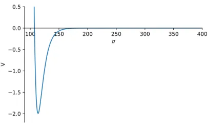
At this point we have stabilized all our moduli. This we did using the assumption that the masses the complex structure moduli receive is large when compared with the mass of the K¨ahler moduli, of which we assumed there was only 1. Thus far we have not broken supersymmetry and there for any vacuum will be supersymmetric. In figure 3.1 we see our potential plotted againstσ. From both figure 3.1 as well as from (3.21) we find that this minimum is an Anti-de-Sitter one as expected.
Figure 3.1:Here we seeV(×1015)plotted forA=1,a =0.1,W0=−10−4
3.7
Constructing dS vacua
following analysis is one of the major point of debate concerning KKLT, we’ll discuss some of this in the next chapter. For now we’ll follow the original paper, [4], in order to compare with their results.
The uplift components we’ll be adding areD3−branes, which we intro-duce as countering additional flux in order to satisfy (3.4). TheseD3−branes add a term to the potential proportional to 1
σ3
† each. For the origin of this
term we refer the reader to [12]. So adding multiple D3−branes means
we need to add D
σ3 to our potential, where D depends on the number of
D3−branes. The factorD depends also on the warp factor at the position of theD3−branes, this ensures that in a warped throat the additional term is small. In principle higher order terms would appear but these scale
quadratically in D, which is exponentially suppressed due to the warp
factor, so we can ignore these.
Here we assume that theD3−branes do not disturb our setup to much. It is this assumption that is at the hart of much of the debates surrounding this model, which again we’ll discuss in the next chapter. So assuming simply adding this term to our potential, implying that our K¨ahler po-tential and superpopo-tential remain effectively unchanged (as side from the additional term in the superpotential) means our potential becomes:
V =eK(Gρρ¯D
ρWDρW−3|W|
2) + D
Im(ρ)3
= aAe
−aσ
2σ2 ( 1 3σAae
−aσ+W
0+Ae−aσ) +
D
σ3 (3.22)
Where we have set τ = 0 for ease of calculation as this just represents
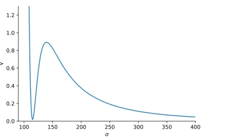
the same degeneracy we discussed in the last section. This potential has again a minimum around the same value as the not uplifted potential. For D ≥ a2A2σ2e−2aσ
6 the minimum is no longer negative. This minimum
however is now no longer global as it is positive and the potential goes to 0 asσgoes to infinity.
†Later papers use 1
σ2 after canceling the warp factor dependence onσin the numerator
Figure 3.2: Here we seeV(×1015)plotted for A = 1,a = 0.1,W
0 = −10−4,D =
3×10⁻⁹.
This new minimum, being positive, corresponds with a de Sitter vac-uum. The value of the potential at this minimum is dependent on the
fluxes and number of added D3−branes and therefor it should be
dis-cretely tunable.
3.8
Stability of dS vacuum, Original
Considera-tions
The uplifted vacuum we found in the last section is as mentioned not a global minimum. This means that we should expect this vacuum to be un-stable, particularly this de Sitter vacuum should decay into a Minkowski vacuum in the decompactification limit of σ → ∞. But this is not neces-sarily a problem for the physical relevancy of the model for if the vacuum is stable enough we may use the model as an effective description of our universe. By stable enough we mean that the time scale of the decay is larger than the expected age of the universe (so larger than 1010 year). On the other hand we’ll also consider an upper bound as argued for in [4]. ”If the decay time is longer thantr ∼eS0, one may need to address the issues
about the consistency of the stringy description of de Sitter space ...”, [4]. Heretr is the recurrence time and S0 = 24π
2
V0 the de Sitter enthropy. This
effects are discussed in [13] and along these lines we’ll analyse the stability of our de Sitter vacuum.
We can think about this decay as a bubble of spacetime tunneling from the local de Sitter minimum in the potential to the lower value of the potential at higherσ. The probability of this occurring is related to the difference in the potential between the two configurations as well as the size of the bub-ble. The bubble after forming has a different vacuum than the surround-ing spacetime. The vacuum of the bubble is lower in energy than the sur-rounding vacuum which will decay in to the lower energy vacuum. The boundary of the bubble mediates between these two vacua, which we can think about as two different phases. The mediation between two phases can be described using an instanton which is what we’ll use here as well.
It is convenient for our description to switch notation to ϕ =
q
3 2ln(σ).
Just as in [13] we’ll look at the probability of decay per volume, P = VΓ, which in the semi-classical limit they find to be approximately:
P =Ae−B¯h(1+O(¯h)) ≈e−S(ϕ)+S0 (3.23)
Where S0 = S(ϕ0) is the action for the initial configuration, in our case
the action at the de Sitter vacuum andS(ϕ)is the Euclidean action for the tunneling trajectory. We consider spherically symmetric decay, that is to say that we assume the volume which decays is spherically symmetric. This means we can use the generalO(4)invariant Euclidean metric:
ds2 =dξ2+ρ(ξ)2dΣ2 (3.24)
Where ξ is the Euclidean time coordinate,ρ(ξ)the scaling factor and dΣ2 the metric of a 3-sphere. The Euclidean action is given by
S =
Z
d4x√g ∂αϕ∂
α ϕ
2 +V(ϕ)−
R
2
(3.25)
This action leads to the following EOM:
ϕ00+3ρ 0
ρϕ
0 = dV(ϕ)
dϕ (3.26)
−ρ
3(ϕ
02+V(
Combining these with the Ricci scalar of the metric
R= ∂αϕ∂
α ϕ
2 +4V(ϕ) (3.28)
means that the action (3.25) simplifies to
S(ϕ) =−
Z
d4x√g V(ϕ) =−2π2
Z ξf
0 dξρ(ξ) 3V(
ϕ(ξ)). (3.29)
The initial state before the spacetime bubble forms corresponds with the limit thatξf → 0. This equal to minus the entropy of our initial de Sitter
congfiguration as formulated in, [14] and [15]. This gives us that S0 is
given by:
S0 =−S0= 24π 2
V(ϕ0)
(3.30)
WhereS0is the de Sitter space entropy.
Thin-wall approximation
The decay of our de Sitter vacuum to Minkowski corresponds with a spe-cial case discussed in [13] of a positive valued false vacuum decaying to a vacuum with zero potential energy in the thin-wall approximation. There for we can use their result for the decay probability which when rewritten becomes
Ptunnel=exp(−
S0
(1+ (4V0
3T2))2
) (3.31)
Where T = R∞
ϕ0dϕ p
2V(ϕ) is the tension of the bubble wall, equivalent toS1 from [13]. For our model we can consider the case that V0 << T2,
which allows us to reasonably expand (3.31) in terms of V0
T2, to zeroth order
this gives us a familiar result
Ptunnel ≈exp(−S0) (3.32)
Which for realistic values of V0 ∼ 10−120 in Planck units, means that the
decay time becomes of the order oftdecay ∼exp(122)satisfying the lower
bound. If we consider first order we get
Ptunnel ≈exp(−S0)exp(64π 2
This means that the decay time becomes
tdecay =trexp−(64π
2
T2 ). (3.34)
Since 64π2
T2 >0 the decay time is exponentially smaller than the recurrence
Chapter
4
Points of critique on KKLT
As mentioned before the Kachru, Kallosh, Linde Trivedi construction, which we examined in detail in the previous chapter, was proposed in 2003. Since it’s introduction it has been one of the bases for the attempts as formulat-ing a de Sitter space in strformulat-ing theory. Other methods exist, such as the Large Volume Scenario, [16], but are beyond the scope of this thesis. It then surprising that after almost 20 year there is still a large ongoing de-bate on whether the solutions proposed by the model are reliable or even exist at all, [17].
Ever since it’s original proposal there have been critiques launched at the model ranging from minute technical details to conflicts with no-go theo-rems, supposedly showing that de Sitter vacua are not possible in string theory.
In this chapter we’ll consider a few of these critiques. In sections 4.1 and 4.2 we go into some more detail for two discussions revolving around the probe-approximation. In the remaining sections we’ll be more brief, only giving a broad outline. This chapter is not intended to be an exhaustive list of all critiques raised over the last two decades. Rather it is intended as a starting point, for the interested reader, outlining some of the more prominent critiques.
4.1
Flattening of the potential due to
backreac-tion
the validity of this approximation is examined.
In principle when we add a supersymmetry breaking object to our anti-de-Sitter solution we should also account for any interactions between this object and our setup, not simply add it’s energy to the potential. We how-ever ignored these interactions in the probe-approximation.
In [19] they give sufficient criterion for the validity of ignoring these inter-actions, namely that the lightest scalar mass times the cosmological con-stant is much larger than unity (relative to the KK scale). This is simply stating that the energy added by the supersymmetry breaking effect, in our case theD3−brane does not have enough energy to excite the moduli. This is necessary for us to consider the moduli as remaining fixed. Which in the notation, we used in chapter 3, this is the following statement:
m2ρ
VAdS2 ≈4a
2
σcr >>1 (4.1)
Where we introduce m2ρ as the mass of the volume modulus squared,
which is approximately m2ρ ≈ a4|A|2e−2aσcrσcr
9 and σcr to indicate the value
of σ at the potential minimum. This condition is not parametrically ful-filled in KKLT models asaσcris not arbitrarily tunable.
So a more in depth analysis of the uplift is needed. For this they use a nilpotent description. This rests on the idea of adding a nilpotent chiral superfield,S, such thatS2= 0, to our set up which will play the roll of an uplift term. Then they proceed to calculate the potential in the same man-ner as before and at the end we putS =0. It is not clear this description is accurate, see [20–22] for a discussion on this. But assuming the approach is valid we can say some thing about the uplift. Adding the nilpotent chiral superfield, S, to our description the superpotential and K¨ahler potential take the form
W =W0+Aeiaρ+e2A
p
24µ3S (4.2)
K =−3 log(2Im(ρ)−SS) (4.3)
Where againSis a degree 2 nilpotent superfield, i.e. S2 = 0. Then calcu-lating the potential after the uplift, then setting S = 0 the potential takes the naive form of
VdS =VAdS+Vuplift (4.4)
description. This term results in an additional term in the potential of the form:
Vcorrections =
e−aσ 12σ2(2
p
24µ3Re(Aceiaθ) +|Ac|2e−aσ) (4.5)
It is clear that if c is small enough this correction term becomes negligi-ble so lets consider where this parameter comes form. It arises from the compactification of the supersymmetry breaking object. In case of KKLT this is a D3−brane in a warped throat, so naively we would expect c to be warped down meaning it indeed would be small enough. There are however a priori possibilities where this warping down does not occur, for example a gaugino condensate which lives outside the throat would have a back-reaction effect which gets blue shifted when considering it’s effect at the tip of the throat. This back-reaction could there for mess with the warping down ofcmeaning the correction term to the potential is not negligible. In that caseVcorrectionswould result in a runaway potential and
we would not have a meta-stabledS vacuum after the uplift, which is ob-viously would be a problem for the validity of the KKLT construction.
4.2
Conifold instability
Again the method of uplifing in KKLT works only if the addition of the su-persymmetry breaking effect doesn’t spoil the anti-de-Sitter vacuum. By this we mean that even though the minimum should get lifted it should
re-main a sufficiently deep minimum. A generalD3−brane placed anywhere
in the compact manifold will not satisfy this condition, it’s contribution to the potential is to large. This we discussed in 3.7 where we argued that
the constantDwas small due to the warp factor adding exponential
of debate on the construction. In this section we’ll examine one of the ar-guments made in this line of thought.
Originally posed in [23], the conifold destabilisation mechanism suggests that the correct way to describe an anti-D3-brane in the throat should take in to account the conifold deformation parameter. This conifold deforma-tion parameter can be thought of as the size of the warped throat. That this needs to be taken into account follows from a calculation done in [24] where they show that the conifold deformation parameter, which we’ll denoteS, is actually lighter, comparable in mass to the volume modulus, than argued for in the original KKLT paper, where it was argued to of or-der R13 same as the complex structure moduli.
This means we can not simply integrate it out and need to treat it as a dynamical modulus. This treatment gives rise to the following potential:
Vks = π 3 2
κ10
gs
(Imρ)3
clog(Λ 3 0
|S|) +c
0gs(α0M)2)
|S|43
−1 | M
2πi log(
Λ3 0
|S|) + iK
gs
|2 (4.6)
Wherecis a constant coming from the warp factor at UV and will be small
c << 1, c0 is a order 1 constant dependent on the warp factor. M,K are the flux quanta andΛ0is the UV cutoff which corresponds with the limit
where the throat is glued to the flux compactification.
From this potential we can easily see that in the limit where S → 0 this potential vanishes which means there is an additional minimum at 0. This
minimum is not taken in to account when one assumes thatS is fixed by
being heavy. In order forSnot to go to zero the potential barrier between the non-zero minimum and zero should be large enough, as the entire
contribution when combined with the term coming from the D3−branes
flattens this barrier. What this means is examined in [24] in the limit where
log(Λ 3 0
|S|) <<
gs(α0M)2)
|S|43
(4.7)
This limit corresponds with a large throat. Then by looking at the values where the non-zero minimum becomes an inflection point they find in terms ofNthe number ofD3−branes the flux quanta int the throat should satisfy:
√
gsM >Mmin Mmin ∝ √
N (4.8)
flux quanta. The tadpole condition provides an upper bound, namely
MK ≤ |Qloc3 | (4.9)
whereQloc3 is the total D3 brane charge from local sources. When we then consider only a single D3−brane and 64 O3−planes these bounds gives us a value for the total hierarchy between the UV cutoff and the IR to be
ΛIR
ΛUV
=exp( 2πK
2gsM
)>0.2 (4.10)
Which would exclude de Sitter vacua with sufficient hierarchy. A nec-essary remark at this point concerning the choice for a single D3−brane and 64 O3−planes is the following. Multiple D3−branes have been ar-gued to give additional contributions to the potential by their internal interactions which would already spoil the vacuum without accounting for the deformation parameter. And the choice for 64O3−planes is some what arbitrary as there exist no known upper limit for the amount of
O3−planes, but most examples in the literature exhibit around this num-ber ofO3−planes.
4.3
IIB backgrounds with de Sitter space and
time-independent internal manifold are part of the
swampland
anal-ysis of different possible corrections applicable to the construction of de Sitter vacua in IIB theory. We’ll not be able to discuss in depth the entire analysis, so we’ll just mention the results relevant to our discussion. The first of these is that in [25] they find that a IIB background with 4d de Sit-ter isometries, a time independent 6 dimensional inSit-ternal manifold, with a metric of the form (4.11), and time independent fluxes are necessarily in the swampland.
ds2= 1
Λ(t)√h(−dt
2+
dx12+dx22+dx23) +√hgmn(y)dymdyn (4.11)
These kind of solutions would include the original version of KKLT as we described it in Chapter 3. However a further result of [25] suggest that certain alterations to KKLT might provide a de Sitter space. This result is that they find that when one allows for the fluxes and internal manifold to be time dependent the resulting theory need not be part of the swampland as previous considerations no longer holds. Such a time dependent setup would have a metric of the form
ds2 = 1
Λ(t)√h(−dt
2+dx2
1+dx22+dx23) +
√
h(F1(t)gαβ(y)dy αdyβ
+F2(t)gmn(y)dymdyn) (4.12)
Whereα,β=4, 5 andm,n =6, 7, 8, 9, which is to say the internal manifold has the structure of a product manifold consisting of a 2d and 4d part.∗ So this argument suggest an alteration to the KKLT model is needed in order to proceed.
4.4
Global compatibility
As pointed out by Liam Mcallister in his talk at Strings 2019, [17], the com-ponents of KKLT are quite well examined seperately. Altough at this point it should be clear that the consensus on the validity of each part is not unanimous in the literature. With this in mind we’ll examine his point anyway. As Mcallister points out we can consider the different compo-nents of the KKLT senario seperately and should pose some questions re-garding these components. Concerning Moduli stabilisation we should ask whether there exit global models with:
• Quantized fluxes giving small classical superpotenial
• Incorporating D7-brane stacks supporting gaugino condensation
• Klebanov Strassler throat regions
And concerning the antibrane uplifting we can wonder whether:
• there is a supersymmetric action that describesD3−branes?
• decompactification is the only important instability coming from the
D3−branes?
• de Sitter can vacua be described in 10d supergravity manner?
4.4.1
Quantized fluxes giving small classical superpotenial
By this we mean that theW0from chapter 3 is indeed<<1 in string units.
This we required in order to be able to neglect all moduli except the K¨ahler as these would be fixed at large mass. Examples of constructions satisfying this condition have been found, for example in [26].
4.4.2
Incorporating D7-brane stacks supporting gaugino
con-densation
The presence of gaugino condensation is an example of a correction that in chapter 3 gave rise to the exponential part in (3.16) needed for theAdS4
vacuum prior to uplift. Although other corrections resulting in a similar term to superpotential might be substituted instead means the existence of gaugino condensation is some sense less crucial. However examples in the literature, such as [27], show that such substitutions while remain-ing interestremain-ing are not necessary. By which we mean that the addition of
gaugino condensation is enough to lead to the AdS4 vacuum. Gaugino
condensation is the most often considered source of these correction terms but other sources exist. So gaugino condensation in particular is not re-quired but there has to be something that gives rise to such a correction term to formulate a anti-de-Sitter vacuum.