and linear programming: an exploration in Ecuador
Caroline Jongkamp Maarten van 't Zelfde Wouter T. de Groot
CML report 163
Land use modelling connecting spatially explicit data and
linear programming: an exploration in Ecuador
Caroline Jongkamp Maarten van 't Zelfde Wouter T. de Groot
Instititute of Environmental Sciences (CML) Leiden University
P.O. Box 9518 2300 RA Leiden The Netherlands
Copies can be ordered as follows: – by telephone: (+31) 71 527 74 85
– by writing to: CML Library, P.O. Box 9518, 2300 RA Leiden, The Netherlands – by fax: (+31) 71 527 74 96
– by e mail: [email protected]
Please mention report number, name and address to whom the report is to be sent
ISBN: 90-5191-142-4
Printed by: Universitair Grafisch Bedrijf, Leiden
1. Introduction... 1
1.1 The context of the study... 1
1.2. Case study area: the Ecuadorian Amazon... 3
1.3. Contents and limitations of this report ... 5
2. Methodology: review of current practice in land use and deforestation modelling.... 7
2.1. Model types... 8
2.1.1. Deforestation models according to Lambin ... 8
2.1.2. Economic deforestation models according to Van Soest ... 11
2.1.3. Multi-agent and Action-in-Context models ... 13
2.2. Towards this report's model on deforestation processes ... 13
Appendix 2-I Description of model applications ... 15
3. Modelling land use decisions of farm households in tropical rainforests: an application for the Ecuadorian Amazon... 17
3.1. The Action-in-Context framework... 17
3.2. Model development: Core structure of the multi-actor land use model... 19
3.2.1. The farm household submodel ... 25
3.2.2. The secondary actor submodel... 40
3.2.3. The tertiary actor submodel ... 47
3.2.4. Model linkages... 49
3.3. Choosing a study area ... 49
3.3.1. The study area: The Northeast provinces of the Ecuadorian Amazon ... 49
3.3.2. Spatial delimitation of the study area... 50
3.4 The farm household submodel applied to the Ecuadorian Amazon... 51
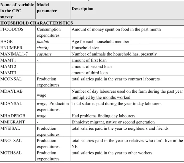
3.4.1. Variables and parameters in the Ecuadorian household model... 54
3.4.2. Model equations for the Ecuadorian household model... 56
Appendix 3-I List of symbols in the core model ... 59
Appendix 3-II List of symbols in the model application for Ecuador ... 62
4. Description of data, data analysis & transformation ... 65
4.1. Data & sources ... 65
4.1.1. Data on household and farm characteristics... 68
4.1.2. Data on the institutional environment and technology... 68
4.1.3. Data on the natural resource base... 70
4.2. Estimating model parameters from the data... 74
4.2.1. Estimating model parameters in the Ecuadorian farm household submodel ... 78
4.3. Results of parameter estimation ... 94
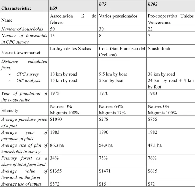
4.3.1. Characteristics of three selected sectors in the Ecuadorian Amazon ... 95
4.3.2. Values of the parameters... 96
4.3.3. Observations on parameter estimations ... 98
Appendix 4-I Description of data sources ... 99
Appendix 4-II Flow charts of GIS data transformations ... 108
Appendix 4-III Avenue script for calculating travel time between farms and markets ... 113
5. Preliminary results from model simulations ... 115
5.1. The Ecuadorian farm household submodel applied to three sectors ... 115
5.2. Model results: discussion ... 118
5.3 Recommendations for further model development... 119
Appendix 5-I GAMS program listing... 122
Appendix 5-II GAMS solve results ... 126
Acknowledgement
1
Introduction
1.1. The context of the study
Maintaining the tropical rainforests is of vital importance for global biodiversity, national economies and the global climate. But the fate of the rainforest is mainly determined by local people and businesses and only indirectly by global policymakers. So how can one nevertheless create a global policy? One that works? These questions underlie the project “Dynamics of Tropical Forest Depletion and Protection” conducted by the Center of Environmental Science of Leiden University. The research was financed by the National Research Programme “Global Change” (NRP) as a follow-up of the research on “Local actors and global treecover policies” (see De Groot and Kamminga, 1995). This research consists of a quantitative and a qualitative study. The current report is the result of the quantitative study on “multi-actor modelling of land use strategies in tropical forest areas”. The results of the qualitative study are documented in a separate publication (Cleuren, 2001).
The problem and the method
The ever increasing, dramatic destruction of the tropical rainforest (see table 1-1) is due in the first place to the people who make the actual decisions about the use of the chainsaw, the fire torch and the bulldozer. These are local farmers, lumber companies, ministries responsible for infrastructure. Behind these primary actors one finds many other actors exerting an indirect influence, such as regional politicians, NGOs and ministries of agriculture. How can a global policy bridge this long chain of cause and effect between the local and the global level? If we do the decent thing and certify all the tropical hardwood on the world market, wouldn’t the deforestation just carry on, but now for the national markets? If tribal peoples were to gain satisfactory title to their lands, wouldn’t they just go and do what the migrants are doing already? If we were to support capacity building in government, would that increased capacity actually be utilised? It might be that the central powers in the developing countries don’t want to maintain the rainforests, which means that capacity won’t make any difference.
Table 1-1. The rate of loss of tropical rainforest Forest area 1990 (106 ha)
Forest area 1995 (106 ha)
Forest loss 1990-1995 (106 ha)
Annual loss ( %)
Tropical Africa 523 505 18 0.7
Effective global policy, pursued in terms of bilateral agreements or via global institutions, thus demands a knowledge of the causal chains running between the global level and what actually happens in the rainforest. The research project on “Dynamics of Tropical Forest Depletion and Protection” attempts to establish these connections. Methodologically, we begin with case studies of the primary occurrences and actors in the forest itself. The method then works its way upward, step by step, along the chains of actors up to the global level. Connections are established by examining the choices that the primary actors can make, and the motivations they may have for choosing a given possibility. We then examine which secondary actors exert an influence on these choices, together with their motivations. In exerting their influence, the secondary actors also have a range of options and motivations, etc. This is called an Action-in-Context (AiC) approach (De Groot, 1992).
NRP I results
In the developing countries it is the nation state that determines how much rainforest can be officially felled. This it does by issuing permits. Every extra tree that is felled is cut down illegally. But that is not in fact a serious hindrance to the lumber companies. An illegal tree is only a more expensive tree because officials and politicians have to be paid off to keep their eyes closed when the tree is felled and transported. There are thus opportunities for forestry policy in combating this informal economy. To this end, one has to act on the motivation of the officials, exercising a more effective control, for instance, or increasing the chances of an official promotion, provided his or her behaviour remains uncontroversial, and giving the official confidence that the policy really does work.
If the state or the lumber companies lay down roads – penetration roads – into the forest, then poor peasants might use them to migrate into the forest. If they do so, the central question becomes one of agricultural transition: will they continue with unsustainable logging, or will they adopt a more sustainable system? That is determined by ‘blind’ markets as well as by government infrastructural policy (feeder roads between the forest margin and the towns), the transmission of agricultural know-how and credit, and the establishment of organisations.
It is often said that governments in developing countries are weak and that capacity building is necessary. But the institutional weakness commonly only holds for the sectoral ministries and the executive services. By contrast, a country’s central power, which simultaneously rules over both the economy and the upper echelons of the central ministries, is anything but weak. This central power determines whether the forest is to remain standing or not, via the many lines that radiate to local levels. This brings us to a global policy aimed at increasing the motivation of these central powers to protect the forests, rather than their capacity to do so. This could be done, for example, by setting up a Global Forest Fund, financed by the Western nations. Such a fund should not pay out for forestry services or promises: it should transfer funds to nations as a whole (in other worlds: to the central powers) per hectare of healthy rainforest. In that way the fund would exert a motivational force at the point where it would have the most effect.
A Global Forest Fund could be financed on the basis of the global value of the tropical rainforest. Funding could be based on ability to pay, on the expected benefits of forest maintenance, on the amount of felling that has already taken place in a given country, and/or on the basis of climate deterioration (CO2 emission). In all cases it would be the Western nations that carry the lion’s share of
payment to the seat of power, and one cannot then control how the money will be allocated from there. But this is exactly what is important for an effective payment scheme: it is essential to motivate the central powers to maintain the forests. Another criterion for effectiveness is the amount paid per hectare. Provisional estimates indicate that an annual turnover of 15 billion dollars per annum could be effective (De Groot and Kamminga, 1995). That’s a lot, but a lot less than the sums mentioned in connection with the stabilisation of CO2 emissions by means of a global climate fund.
1.2. Case study area: the Ecuadorian Amazon
In the framework of the present project, field research to the Northeast of the Ecuadorian Amazon has made clear how the mechanism of tropical deforestation operates there. The study area was chosen in the provinces of Napo and Sucumbios; in the region around Coca1. This area is in the heart of the
lower rainforest region. The discovery of oil thirty years ago in this area of Amazonian jungle has wrought a radical change in the region. Western oil companies posses concessions over large areas of rainforest and are the pioneers of forest exploitation. They use heavy equipment to lay down roads and to get the oil wells into production. This is accompanied by the destruction of areas of rainforest and pollution of soil and water by poisonous drilling fluids and oil. In their wake follows an army of impoverished colonists and Quichua indians, in search of land. These are the primary actors in the deforestation and they have established themselves along the oil roads over the last thirty years. Most of them lead a marginalised existence on their plots of low fertility land where they cultivate manioc, plantains and rice for their own consumption, and coffee for the market. The area is “backward” in the sense that the availability of health care, education and other services is far below the standards in the rest of the country. Despite the harsh living conditions, the region is still attractive to colonists because of the employment possibilities in the oil business and the relative abundance of land.
Large cattle ranches are hardly found in this area due to climatic conditions, inadequate knowledge and capital, and poor grazing lands. The peasants do not fell large areas of forest; rather, they work a few hectares to produce their own food, eventually felling the most valuable tree species in the remnant forest for sale to the lumber companies. Forest clearing is slower than in other regions in the Amazon. The year-round rainfall makes it difficult to perform slash-and-burn clearing. A common procedure is the so-called slash-and-mulch method, by which the vegetation is not burned, but cut and left to rot. The rather slow pace of deforestation gives room for interventions geared towards sustainable land use practice, provided that the farmers have the necessary incentives which are vital if they are to develop new and sustainable initiatives.
The fate of the Ecuadorian Amazon is to a large extent governed from the capital city, Quito, where the central power views the region merely as an area for the extraction of oil. Though much criticized for its environmental effects, the oil sector can not be denied for its important contribution to national living standards, public budget and foreign exchange. Oil extraction still continues, and so does the construction of new roads into the forest. Only if this process can be halted is there a chance that the process of deforestation can in fact be controlled. However, the lack of political will is a matter of serious concern. The Ecuadorian case study confirms the crucial role played by the central elite in deforestation. The key towards sustainable forest management should therefore be searched in economic stimuli that can change this group’s behaviour.
The remainder of this report describes the interaction between the primary, secondary and tertiary actors in deforestation. We have chosen for a modelling approach which makes it possible to quantify the underlying processes and motivational factors. The model was designed with the purpose to evaluate the effect of policy scenarios which slow down the deforestation process. Chapter 2 contains an overview of current research in land use and deforestation modelling. It concludes with observations on modelling techniques that we will employ in our study. Chapter 3 further develops the model for three major actors: the farm household as the primary actor responsible for deforestation; the government as the secondary actor influencing household strategies; and an international organisation which represents the (western) donor community. The model incorporates methods of socio-economic research and GIS techniques. A reduced version of the model is presented for a specific study area in the Ecuadorian Amazon region. Chapter 4 continues with a description of the data analysis required to perform the model calculations. Finally, the Ecuadorian model is tested with data on farm household behaviour in the study area connecting the GIS-data with the linear programming using the GAMS software (chapter 5).
2
Methodology: review of current practice in land use and
deforestation modelling
Why modelling?
The choice for a modelling approach was made on the one hand because of the complexity of actors’ decisions and their interactions, and on the other hand because of the possibilities that quantitative modelling offers for policy simulations. The causal linkages between actors’ behaviour and the motivational factors are the basis for the design of the model equations. After the basic structure of the model has been designed, the model can be validated in a local context. The validation process requires that a thorough data analysis is made, and parameters are estimated to specify the sensitivity of the actors to the local circumstances.
The modelling procedure follows the Problem-in-Context and Action-in-Context frameworks as developed by de Groot (1992). The Problem-in-Context (PiC) approach starts from the environmental problem, in casu destruction and degradation of humid tropical forest. After describing the problem, the next step in PiC is to describe its context. Problematic actions, which are, in their turn, caused by decisions of actors, and the factors and motivations that facilitate these decisions cause the environmental effect.
This chapter has been written in an early stage of the project as a preparation for the quantitative modelling of land use in tropical forest areas. Many others have used modelling techniques for similar purposes as we do. The integration of both physical and socio-economic factors in quantitative models is – methodologically speaking - the most challenging part of our research because there is little experience in this field. Even though our focus is on the human driving forces of deforestation, we have been determined from the beginning of the research to include geo-bio-physical factors in the modelling, and to do that to the best of our knowledge. In the real world there is a day-to-day interaction between human and physical factors and our aim was to develop a powerful (modelling) tool which is sufficiently robust to improve our insight in the nature of these interactions.
2.1.
Model types
This chapter is mostly based on three studies which together give an overview on the type of models that have recently been used to analyze the human causes of deforestation. The first is Lambin (1994), the second Van Soest (1994), and the third is Lonergan and Prudham (1994). This section merely reflects the findings of these authors. Lambin focuses on searching a complementarity between monitoring changes in land-use/land cover by remote sensing and the modelling of change processes. As such, the models that he discusses are necessarily spatial. In fact RS and modelling efforts tend to come together only sparsely, yet its combination is one of the most promising "novelties" within the field of GIS.
Lambin is quite brief in his discussion of economic models. This gap is nicely filled in by Van Soest, who focuses particularly on economic models. Lonergan and Prudhan discuss in particular lexicographic goal programming and multi-criteria analysis.
2.1.1. Deforestation models according to Lambin
Lambin distinguishes (Lambin, 1994, page 22) three types of models for processes of land-use and land-cover change: empirical, mechanistic and system models. Empirical models are based on observed relationships between variables. Mechanistic models are based on the modeller's knowledge of the underlying processes by which the system operates. Parameters must be estimated from data, and the suitability of the equations needs to be verified by observations. System models take into account several complex, interacting processes. These models are often difficult to validate and very computer intensive. The models can be made spatially explicit to predict changes in spatial structure of the landscape and map the flows that occur between locations. After these and a few more general remarks, Lambin proceeds to the description of more specific model types:
1. Markov chains:
In Markov chain models, probabilities are assigned to the transition from state i to state j. For land-use studies, the states of the system are defined as the amount of land covered by various land uses, as percentages of the area of each landscape unit. The transition probabilities are stationary over time. The probabilities can be statistically estimated from a sample of transitions which actually occur and can be observed during a certain time interval. If aij indicates the transition between state i and state j, then the transition probabilities pij are estimated as:
pij = aij/ SUMjpij
In the long run, the predictive power of the Markov chain in its basic form is quite limited because of its assumption of stationarity. It does not explain the underlying causes of the transition, nor does it take into account any possible changes in the underlying causes. In order to address the underlying causes, it is possible to incorporate the contribution of exogenous or endogenous variables to the transitions. Hence, pij could be estimated as a function of the variables X1, .., Xn : pij = f(X1, .., Xn).
3. (Linear) regression models postulate a (linear) relationship between the dependent variable (Y) and independent variables (Xi) in the form:
Y = a0 + a1X1 + a2X2 + .. + random error
where the ai are the regression coefficients, usually estimated by the ordinary least squares (OLS) method. Regression analysis can be conducted by cross-sectional analysis or by panel (time series) analysis. Lambin sees a weakness in the application of cross-national analysis applied to a wide range of countries in very different situations. He therefore makes a plea for preliminary stratification of the globe into homogeneous zones, on the basis of geographical, ecological or socio-economic criteria. Another weakness of cross-sectional regression models is that they do not allow for cross-boundary effects.
Many examples exist of studies which used regression analysis to establish relationships between deforestation and explanatory variables such as population density, road density, soil productivity, etc. Lambin mentions a few. Among them is an interesting study on deforestation in the Philippines (Kummer, 1991), which demonstrates the role of roads in opening up the forest area for migrants. Another - more comprehensive - overview can be found in Brown and Pierce (1994).
4. Spatial, statistical models combine remote sensing, geographic information systems and statistical methods. They offer cartographic projections and establish correlations between the spatial occurrence of land cover (derived from RS data) with landscape and locational attributes (e.g. from aerial photography). The models deal primarily with the question of which areas are most susceptible to deforestation. A dependent variable, like the "change in land cover" is related to a number of independent variables such as slope, elevation, degree of fragmentation of the forest, proximity to housing, and proximity to roads and streams.
5. Models of population pressure, agrarian change and deforestation. Population pressure increases the demand for food, and hence the demand for arable land. This forces people to use forest land for cultivation. On the other hand, people may use techniques which increase the productivity of the land which is currently available.
This type of models are rather crude and have limited applicability on a local scale. They only explain agrarian changes which are driven by population growth. Non-demographic causes of deforestation are not taken into account. The models are mainly qualitative, explanatory, non-predictive and non-spatial.
6. Models of peri-urban land-use change.
7. Econom(etr)ic models
A common econometric approach is to specify and estimate supply and demand functions of market goods. Examples of such "market goods" are forest land, labour, forest products, or agricultural cash crops. The standard estimation technique is ordinary least squares regression. Lambin further mentions optimisation theory, partial equilibrium modelling, and general equilibrium modelling.
The economic models described by Lambin are not explicitly spatial, but he assumes that there is a clear potential for developing spatial economic models of deforestation processes, using concepts from location theory and from regional science.
A more elaborate sub classification of economic models is given by Van Soest (1994). See the next section.
8. Ecosystem simulation models:
Ecosystem models emphasize the interactions among all components that make part of the system. The dynamic behaviour of the system is then studied through simulation experiments with the model. The simulations can be used for analytical and for predictive purposes. Lambin mentions the IMAGE model, developed by RIVM, as an example of this type of models. Lambin considers it a prerequisite for the development of this type of models that the processes and mechanisms of deforestation in a given situation have been thoroughly investigated, for example through detailed field studies.
Lambin considers it a disadvantage that most ecosystem models treat the system as spatially homogeneous. Spatial heterogeneities could be introduced more explicitly (see under 9 below), but this is limited by computational constraints on the number of flows to be estimated between spatial units.
9. Dynamic, spatial simulation models:
This model type is an expansion of the ecosystem models mentioned above. They include (i) the spatial heterogeneity of the land surface and (ii) the processes of human decision-making underlying changes in land uses. In this type of models, the flows between adjacent grid cells are explicitly taken into account. Lambin mentions two examples of these models, which are both spatially explicit actor-based models. The first, developed by Wilkie and Finn (1988) applies to the equatorial forest in Zaire. The second, the DELTA model (see e.g. Dale et al, 1993), is developed at the Oak Ridge National Laboratory and has been used to contrast two land use systems in Rondônia, Brazil.
Types of models
Issues to be addressed Empirical models Mechanistic models System models
Why? Regression models Population pressure & Economic models
Ecosystem models &
Dynamic spatial simulation models When? Markov chain &
Logistic function model
-
Where? Spatial, statistical models
Models of peri-urban land-use change
Dynamic spatial simulation models
Source: reproduced from Lambin (1994), page 97, table 1
Lambin advises to start building stochastic models characterized by a simple structure, and to progressively elaborate those models. Though I fully agree with his idea to incorporate stochastic elements, I would rather consider to leave these out at the first stage of modelling, and to incorporate them in the elaboration phase. The value of stochastic elements will be evident also in case of deterministic processes, "to represent unpredictable factors associated with deforestation" (quote from Lambin, page VII).
2.1.2. Economic deforestation models according to Van Soest
Van Soest (1994) discusses four model types which are commonly used in applied economic analysis. He distinguishes statistical analysis, input-output models (and Social Accounting Matrices), linear programming models and general equilibrium models. Statistical models have been mentioned already in the previous section, therefore I will not repeat the discussion here. I will briefly describe the other three.
10. Linear programming models
The essence of linear programming models is the constrained optimization of an objective function. The objective function specifies the preferences of a decision maker. An example of an objective function is to maximize profits in a production process. The constraints deal with matters such as the production capacity and the availability of labour.
Maximize: c1X1 + c2X2 + ... + cnXn Subject to the constraints:
a11X1 + a12X2 + .... + a1nXn # b1 a21X1 + a22X2 + .... + a2nXn # b2 . . . am1X1 + am2X2 + .... + amnXn # bm
Van Soest mentions the TROPFORM model as an example of a linear programming model which is built to simulate possible trends that affect deforestation on a global scale (see Jepma, 1995). The model focuses on the production and trade of wood products.
Related model types are the non-linear programming model, which has non-linearities in the con-straints or in the objective function, and the integer programming model, which requires that the optimal values of the decision variables have integer values.
11. Input-output models and Social Accounting Matrices
Input-output models are built on so-called input-output tables. Generally, these tables are composed for national economies, or for regions. These tables specify the technical relationships between quantities of inputs and quantities of outputs in the production processes of the economy. The output produced in one sector may be used as an input in another sector, and so on. The quantities of goods required as inputs together constitute the intermediate demand. Not all outputs are used in the production process, part of it is directly consumed. This is called the final demand. Based on the input-output table, the model can calculate for any value of the final demand how many intermediate goods need to be produced. Therefore, it is a useful model to analyze how changes in one sector induce changes in other sectors.
A Social Accounting Matrix (SAM) is an extension of the Input-Output table to include social effects of production processes. For example, forest degradation can be included as one of the social effects. With the help of the SAM, it can be seen which of the activities (as specified in the input-output table) inflicts most damage on the forest land. Because all the interlinkages between the sectors are taken into account, it measures not only the direct effects, but the indirect effects as well.
A disadvantage of the I-O and SAM based models is that it assumes fixed relationships between inputs and outputs, even if major changes in demand occur. A second disadvantage is that it assumes that supply adjusts perfectly to demand.
11. Computable General Equilibrium (CGE) models
Further removed from economic science but still largely applying rational choice theory, multi-agent and Action-in-Context approaches stress the needs and opportunity to causally relate various actors with each other, e.g. to explain tropical deforestation.
12. Multi-Agent Modelling (MAM)
Multi-agent models usually work with relatively simple actor equations, focusing rather on the system-level effects or the interplay of may of such actors.
13. Action-in-Context (AiC) modelling
Responding to the need to link the causal strength of actor-based methodology with higher-level cultural and structural variables, De Groot (1992) developed the Action-in-Context framework. One of its characteristics is that actors are related to other actors through influences on these actors' options and/or motivations for action. Thus, 'actor field' structures can be developed in which direct ('proximate', 'primary') actors are causally connected to higher-level ('secondary', 'tertiary' etc.) actors. See also De Groot and Kamminga (1995) for tropical forest examples.
2.2.
Towards this report's model on deforestation processes
Many of the models described above could be useful to our own modelling efforts. The most appealing model type is the one which Lambin denotes with the dynamic, spatial simulation models. They have everything that could be needed: actor-based hence causally oriented, spatially explicit, linked with remotely-sensed data, stochastic simulation, ... When aiming towards such a comprehensive model, we could use a number of the other model types as well. For example, regression analysis can be used to estimate parameters which are used as inputs in a spatial simulation model. Out of the above lists of model categories I will mention a few which I consider potentially useful for our own modelling efforts:
• dynamic spatial simulation models: the most powerful integrated modelling type
• regression models: useful to estimate parameters and distribution functions
• spatial statistical methods: useful to estimate parameters of an evidently spatial nature
• von Thünen's model: to explain the behaviour of actors vis-à-vis distant markets
• linear programming models: useful to model the decision process of an actor if constraints play an important role
This list is not meant to be exclusive, other model components may be useful as well.
flexible, and have explanatory power in a local and global sense.
The development of the model is a stepwise process. It is built up similar to the action-in-context approach, starting from the strategies of the primary actors and gradually proceeding to the secondary and tertiary actors. Of course, we need to do a lot of testing and validation with data in between. The modelling efforts and the improvement of our understanding of mechanisms is an interactive process. On the one hand modelling is nothing more than formally describing what we already know, on the other hand, the calculations with models and the outcomes provide a check on whether we actually understood the logic of what is taking place. In this way, it is a steering instrument to guide the collection of data in the field. The knowledge gained in the field should help to improve the models. Data from secondary sources also provide an indispensable input in the improvement and validation of the models.
Description of model applications
Allen
The model by Allen (1985) is briefly discussed in Jepma (1995, p.71). It is a forest conservation model of the Dodoma region in Tanzania, used for comparing policy scenarios aimed at the transition from deforestation of public forest areas to the use of plantation wood. The model, a multi-goal programming model, generates an optimal combination of efficient wood production, allocation of labour and conservation of the forest.
CLUE
The CLUE model (Conversion of Land Use and its Effects; Veldkamp and Fresco, 1996, Schoorl et al., 1997) is a spatially explicit, multi-scale land-use change model. It was built up through regression modelling, where the potential driving forces are included by stepwise inclusion according to their performance in the regression model. Applications and further model development of the CLUE model are described in De Koning, 1999; Kok, 2001; and Verburg, 2000.
Hassan and Hertzler
Hassan and Hertzler (1988, discussed in Jepma, 1995) describe a dynamic programming model for Sudan in order to develop an optimal policy to control forest exploitation as a source of energy on the one hand and desertification on the other hand. The model uses real prices of fuel wood, which take into account the costs of logging for future generations.
IDIOM
IDIOM is a global simulation model used by Jepma (1995) for scenario analyses. The IDIOM model integrates TROPFORM (see below), SARUM (a global simulation model developed by the Systems Analysis Research Unit in 1978) and a land use module. SARUM divides the world in 10 geographical, economic and/or political regions (North America, Tropical Latin America, Rest of LA, etc.).
Image 2.0
Image consists of a number of modules, one of which is the carbon cycle module. This module, on its part, contains a deforestation module as a submodule (Rotmans, 1990, section 3.7). The submodule takes into account the following processes:
• permanent agriculture
• shifting or pioneer cultivation
• cattle breeding
• logging
• fuelwood gathering
• industrial projects (in Amazonia only)
TIMPLAN
A sector simulation model developed by Gane (1986, described by Jepma, 1995) in order to determine the best strategy for forest development on a national level. The model generates projections of the future demand and supply of wood, costs and benefits of the forest sector, earnings in foreign currency and benefits for the national economy.
TROPFORM
This global model describes several factors determining land use and leading (eventually) to deforestation (described extensively in Jepma, 1995, pp. 71-82 and Blom et al., 1990). The emphasis is on the logging industry. The model consists of the following modules:
- consumption module (assumption: all demand for wood products is met) - spatial allocation module (linear programming)
- standing volume module - growth reserves module - deforestation module
The deforestation module considers three types of land use:
- farmland or agricultural land (meets consumption demand for food) - forest
3
Modelling land use decisions of farm households in tropical
rainforests: an application for the Ecuadorian Amazon
This chapter discusses a modelling framework for the analysis of land-use decisions in tropical moist forest areas, with an example from the Northeast Ecuadorian Amazon. The core structure of the model is a multi-actor modelling framework. It takes into account the interaction between primary actors (e.g. the farm households), the secondary actors (e.g. the oil companies and the government) and the tertiary actors (e.g. the international donor community). In section 3.1 it will be explained how the decisions of the actors influence each other through a presentation of the Action-in-Context framework. Section 3.2 discusses the development of the quantitative model. The result is a framework for what we call the “core model”. The core model is built up from a number of submodels which are linked to each other. Each submodel deals with the decision-making process of one type of actor. Section 3.3 contains a geographical delimitation which results in the choice of a particular study area in the Ecuadorian Amazon. Then, in section 3.4. we will present an example of the household submodel as it was applied to the land use decisions of a farm household in the Ecuadorian Amazon.
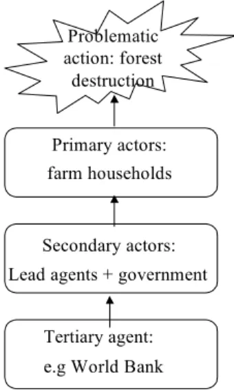
3.1. The Action-in-Context framework
Figure 1. Linkages in the Action-in-Context framework
Problematic action: forest
destruction
Primary actors: farm households
Secondary actors: Lead agents + government
Tertiary agent: e.g World Bank
3.2. Model development: Core structure of the multi-actor land use model
The model development takes the same steps as the Action-in-Context framework: from the primary actors up to higher levels of influence. We can structure the model development along the following steps, which need not necessarily be taken in this exact order:
a) Define the decision-making process for each actor b) Identify the available data and collect additional data c) Choose the unit of analysis and link this to a spatial unit d) Design model structure and equations
e) Estimate model parameters
f) Run the model for a baseline scenario
g) Evaluate the model results for the baseline scenario
h) Design and implement model experiments for alternative scenarios
Steps a)-d) will be discussed in this chapter. Step e) is the subject of chapter 4. Steps f)-h) will be discussed in chapter 5.
Ad a) Define the decision-making process for each actor
Before the behaviour of the actors can be modelled we will first give a more formal description of the decision-making process of each actor. The knowledge on these decision-making processes is obtained from theory and (for specific study areas) from field research, and results in a description of “hypothesized behaviour” of the actor at stake. This hypothesized behaviour is necessarily a generalization of actual behaviour and is the basis for a set of assumptions which together describe how the actor responds to the motivational factors. The assumptions might be verified in the field by means of survey techniques commonly applied in the social sciences, such as sampled surveys or even in-depth interviews. This, however, is quite expensive and often impossible on a limited research budget. In our research we based our assumptions on actor behaviour on “light” surveys and a relatively large component of secondary sources. In this way, a crude understanding was obtained on actor behaviour with respect to the depletion or protection of the rainforest.
First we will formulate a number of assumptions which have been derived from the literature on farm household economics and on deforestation (e.g. Ellis, 1988; Singh, Squire & Strauss, 1986; Rudel and Horowitz, 1993; Brown and Pierce, 1994; Jepma, 1995). 2
The assumptions regarding the primary, secondary and tertiary actors
The primary, secondary and tertiary actors are defined as follows: 1. The primary actor is the farm household3
2. The secondary actors are a lead agent (like a logging company or the oil sector) and the government. The government may have to be split into several divisions, depending on whether these function as relatively autonomous institutions.
3. The tertiary actors include international agents involved in policymaking (e.g. World Bank, international environmental movement), representatives of the international donor community (e.g. World Bank), and trade institutions (e.g. WTO, ITTO). Typically, international institutions are involved in more than one of these fields.
The assumptions regarding the primary actors: farm households
The following assumptions define the livelihood strategies of farm households in tropical forest areas. They are not meant to describe households in their full diversity and complexity, but they describe the major components of their land use decisions.
4. The objectives of the farm household include at least (i) food consumption and (ii) asset accumulation.
5. It is assumed that the household prefers family food consumption up to a ‘basic needs level’ to accumulation of other assets.
6. It is assumed that farm household decisions can be represented by only one decision-maker. Though this assumption may be unrealistic for some households, it is often a necessary approximation of household decision-making if interaction between several decision-makers within a household is complex and impossible to identify properly.
7. The household makes both operational decisions (with a short-term effect) and strategic decisions (with a long-term effect). For strategic decisions several years may elapse between the decision and the moment that the effect on the household objectives is fully accomplished. Examples are the growing of perennial crops and the clearing of forest land. Expectations on future events (e.g. price development, land tenure perspectives) play an important role in these strategic decisions. Operational decisions are defined as decisions with effects exclusively or predominantly within one year, whereas strategic decisions have effects over the years. We further assume that the household has a planning horizon of 10 years and that strategic decisions take effect within this planning period.
8. Food consumption is satisfied partly by home produce and partly by purchases on the market. The degree to which the farm household is involved in market transactions depends on access to markets as well as on various price and cost factors. The farmer takes these factors into account while making decisions on the production and marketing of food products.
9. Income generating activities are categorized as farming, animal husbandry, extraction of forest products and non-farming income generation.
10. Each of these income-generating activities is subdivided in more specific activities; each has different effects on the household objectives and on the environment (in casu state of the tropical forests). For farming, we need at least a distinction between food crops and cash crops, as well as annual and perennial crops. For animal husbandry grazing densities are important, as well as its effect on asset accumulation. Extraction of forest products can be done farm (if there is on-farm forest) and off-on-farm. We assume that the extracted forest products (e.g. wood) are sold in the market. The effect of the extractive activity on the state of the forest, that is degradation from primary to secondary (logged-over) forest, is taken into account. Non-farming activities include at least off-farm wage labour. Non-farming income-generating activities are taken into account for their effect on the household budget and on available family labour.
The assumptions regarding the secondary actors: lead agents and government
12. The lead agent (see Rudel, 1993) is the actor that enters the forest for commercial motives before households begin to settle. The lead agent builds roads and hires labour. In this way, the lead agents facilitate the settlement procedure. The lead agent is normally active in extraction of natural resources, such as wood or mining products. The objective is profit maximisation. Whether the company has a short-run or a long-run perspective can not be stated in general.
13. The government may also be a lead agent by facilitating the settlement of households, but not necessarily so. It typically has multiple and conflicting objectives, such as protection of nature and generation of foreign exchange or tax revenues. We assume that the major objective of the government is to keep its position in leading the country. All governments have a budget that they use to effectuate policies in the forested areas. Secondly, all governments apply laws, rules and regulations to effectuate policies. The government is regarded as one single decision-maker, who co-ordinates the conflicting objectives of its departments.
14. Other secondary actors may be added depending on their role in a particular study area.
The assumptions regarding the tertiary actors: international agents
The identification of tertiary actors is particularly complex because many international organizations claim to have similar objectives. The World Bank, for example, is primarily an institution that promotes economic development. More and more this objective has bended to make place for a concern with nature and environmental issues. The key objective for the World Bank (as well as for many other international institutions) is now “sustainable development”. Actually, this term is just a way of stating that multiple objectives are pursued, where the objectives may even be in conflict with each other. The various organizations each have a particular focus, but it is common that their policies are the result of a complex set of conflicting objectives. For this research we consider a single hypothetical international agent.
15. The tertiary actor is a hypothetical agent, called “International Organization for Sustainable Development”, abbreviated as IOSD. Its main objective is “sustainable development”.
16. It is assumed that the IOSD has a considerable amount of money available originating from contributions of wealthy nations.
17. The decisions of the IOSD are restricted by external rules such as limits imposed by sovereignty regulations, trade agreements etcetera. These restrictions have to be specified depending on the relevant factors in the particular study area.
Ad b) Identify the available data and collect additional data
Both qualitative and quantitative data are required to fill in the details concerning the actors’ behaviour. The hypothesized behaviour described by the assumptions above defines only the basic rules along which the actors take decisions. The model and data analysis should point out to what extent the environmental effects are explained by changes in the motivational factors. The search for data then starts with a choice of a study area. Ideally, the study area is chosen such that (a) the dynamics in the study area can be seen as representative for processes in other forest areas, and (b) a large variety of data is available on the natural resource base, the institutional environment, the population and actors’ behaviour. In other words, the area must be “interesting” in the sense that conclusions can be projected and used for policy analysis beyond the boundaries of the study area. The availability of data is often a limiting factor. Deforestation is a process which takes place over a long period of multiple decades. Historic information from the early settlements as well as from more recent times is valuable to help understand the changes that take place, and at what speed they are taking place. First an inventory is made of the available secondary data. Also, additional data collection may be required to fill in gaps in the secondary data. Maps of the area may provide valuable information. Data from different sources must be combined and related to each other. Data bases, statistical techniques and GIS tools are required for this procedure. Qualitative studies and field visits are required to understand the actors’ behaviour with regard to the forest. For the primary actors the use of forest land is an integrated part of the livelihood strategies, therefore the whole livelihood strategy is subject of study. The purpose of the data collection and analysis is to get a more comprehensive and detailed knowledge on the actors’ strategies. This knowledge is the basis for the development of the actor submodel.
The process of data collection and analysis is illustrated in Chapter 4 for a study area in the Ecuadorian Amazon. For now we will proceed with the discussion of developing the “core model structure”.
Ad c) Choose the unit of analysis and link this to a spatial unit
Units of analysis
We have chosen the farm household as the unit of analysis for the decision-making of the primary actors. An important aspect is the question “Who actually takes the decisions?” Can the household be considered as a homogeneous unit of decision-making? For many decisions the household level can be regarded as appropriate in this respect, for others a higher or lower level is more accurate in practice. A higher level of decision-making might be a village or a group of similar households. Within the household, individuals may take decisions independent of the others. Women are mostly responsible for family health and nutrition, whereas men usually take the primary responsibility for production related decisions. As long as the goals and strategies of different household members are not conflicting, there is no harm done to reality if we treat the household as a collective unit of decision-making. The household is the unit which is distinguished by the “common roof, common pot”.
question which needs to be addressed in a study of the local situation. It needs to be identified who takes the “government-decisions”; and – if there are multiple decision-makers – to what extent their motivations and instruments coincide or differ; and to what extent they have a different influence on the options and motivations of the farm households with respect to land use.
The tertiary actor, the hypothetical “International Organization for Sustainable Development” (IOSD) is also considered as one single decision-making unit, and, accordingly, as a single unit of analysis.
Geo-referencing of the unit of analysis
The geo-referencing of the unit of analysis is necessary in order to perform spatial analyses. If the location and size of the household plot is known, and can be identified on a map, the unit of analysis for the primary actor can be linked to a spatial unit.
The unit of analysis for the secondary actor coincides either with the whole study area, or a geographical subdivision depending on whether the influence of the decision-maker(s) can be considered as homogeneous over the whole study area. The tertiary actor has an aggregation level higher than the whole study area, hence the spatial unit can be chosen as the assembly of the tropical forest areas all over the world.
Data with a spatial component are stored and analysed in a GIS. We have chosen to use SPANS-(GIS)-software for most of the spatial data. The SPANS-software is a so-called “quadtree-GIS”; a raster-oriented storage format which can easily be disaggregated or aggregated if a higher or lower level of detail is needed. This may be useful if data need to be exchanged with other models. The choice of a raster storage format (instead of a vector format) for the basic spatial unit has the advantage that each unit (or grid cell) has a standard size and shape. Data from different data-themes can easily be combined and compared. For example, data on land cover and on household characteristics can be stored with the spatial unit to which they belong. However, for some types of data analysis the use of a raster format can be a disadvantage if the data take different shapes. For example, one of the factors influencing household decisions is the distance between the farm and the nearest market. For an accurate calculation of the distance based on road network data it is better to use a vector storage format instead of a raster format. In this particular case, we have used vector-oriented GIS-software (ArcView) for the analysis of the road distances. The results of the analysis were converted to the basic spatial unit for later use in the mathematical model4.
The role of the spatial analysis in the modelling procedure is twofold: first the spatial (and non-spatial) data are analysed to generate input for the mathematical model. Secondly, the output generated by the model is used for geographical presentations by making use of the spatial units and their locations in the study area. In this way, we achieved an integration of spatial and non-spatial methods of analysis.
Ad d) Design model equations, estimate model parameters
The knowledge obtained from the data and literature is used for the mathematical formulation of the actor submodels. Each actor submodel describes the decision-making process of an actor. First we will make some general observations on how decisions are being made. A decision maker can be seen as a person who wants to maximize “utility” while being faced with a set of instruments which he can use to obtain his goals. “Utility” is an abstract term which denotes the whole set of material and immaterial values that the decision-maker judges as important for himself and the “unit” that he represents. The most obvious material value is wealth (accumulation of assets). Examples of immaterial values are good health, access to schooling for children etc. The decision-maker weighs all these objectives to the best of his knowledge before he takes actions. He has to take into account all the instruments that he has available. For example, a farmer who has to take planting decisions for the next growing season will take into account the “values” of earning money, as well as the discomfort of spending labour time and the limited land that he has available.
The family of mathematical programming models is particularly useful for describing these kind of actor decisions. For each decision-maker they consist of an objective function and a set of constraints. The objective function is a combination of the goals that the actor wants to maximize, for example the accumulation of assets. The constraints together describe the set of options and limiting factors, formulated as conditions that need to be satisfied. An example of such a condition for a farmer is that the planted area can not be larger than the total amount of land that the farmer has. This type of conditions (constraints) can be formulated in mathematical terms as equalities and as “less-than” or “greater than” inequalities. Together, the objective function and the constraints describe the decision-making process of the actor.
Within the family of mathematical programming models we consider the linear programming (LP) model suitable to describe the decision-making of our actors. In the linear programming model5,
the objective function is a linear combination of decision variables6, which can be seen as the instruments that the decision-maker has available.
Steps e) to f) from the estimation of model parameters to the evaluation of the model results for the baseline scenario will be discussed in chapter 4 and chapter 5. Step h), the design and implementation of model experiments for alternative scenarios is mainly left for future research because of the limited scope of this report.
5 Mathematical programming models can be subdivided into linear and non-linear programming models. In
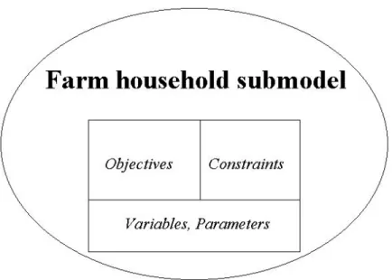
3.2.1. The farm household submodel
We start out with the submodel for the primary actor: the farm household. The major questions which the model addresses are:
1. For each spatial unit, what is the farmer’s expansion strategy towards increasing crop land and pasture at the cost of (primary) forest?
2. On the basis of the major motivational factors, can we identify spatial units currently under forest that are likely to be colonized by farmers in the near future?
Figure 3- 2 Components of the farm household submodel
Variables and parameters in the household submodel
The decision variables in the household submodel represent the choices of the decision maker. The farmer needs to make decisions on the activities that he can choose from. In general we can say that the decision describes the choice of the allocation of inputs among a number of alternative activities. The values of the decision variables are unknown on beforehand, and need to be calculated by the model.
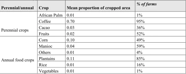
Activities, decision variables, and inputs
We have defined the categories of farm household activities in Table 3-1. The Table serves as a guideline which represents the most common farming activities; the list of activities may need to be adapted to describe a local context.
Table 3-1. Activities in the farm household submodel
ON-FARM LAND USE ACTIVITIES, E.G: - food production, annual crops - food production, perennial crops - cash crop production, annual - cash crop production, perennial
- land conversion (e.g. forest to arable land) - animal husbandry
- on-farm logging
- expansion through buying or occupying land - disposal of land through selling or abandoning OFF-FARM INCOME GENERATING ACTIVITIES, E.G.: - off-farm logging
- off-farm labour
NON-INCOME GENERATING ACTIVITIES, E.G.: - consumption of farm products
- food expenses - non-food expenses - saving/investment
Non-income-generating activities are important too, because they compete with the other activities for the use of inputs. The list of activities is not meant to be exact because local situations may require a somewhat different categorization. In the remainder we will refer to activities with the index i. Occasionally we make use of subsets which are denoted as {land use activities}, {off-farm income generating activities}, and {non-income generating activities} according to the categories in Table 3-1. The whole set of activities is denoted by {all activities} (see also Appendix 3-I).
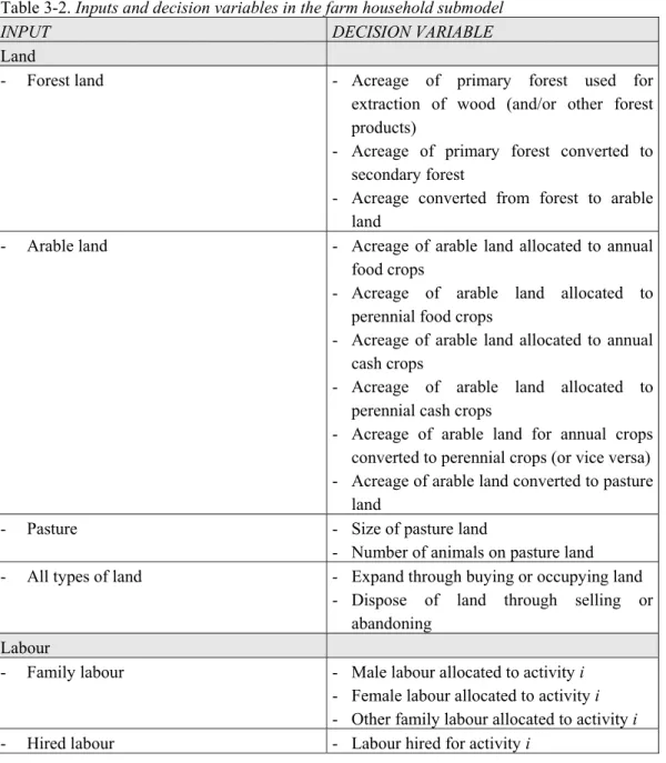
Inputs include the broad categories of land, labour, and capital. These can also be subdivided into smaller categories relevant to the farm household (see Table 3-2). Again, the level of detail and the number of classes for land, labour and capital can be adapted according to the requirements of a local context.
Table 3-2. Inputs and decision variables in the farm household submodel
INPUT DECISION VARIABLE
Land
- Forest land - Acreage of primary forest used for extraction of wood (and/or other forest products)
- Acreage of primary forest converted to secondary forest
- Acreage converted from forest to arable land
- Arable land - Acreage of arable land allocated to annual food crops
- Acreage of arable land allocated to perennial food crops
- Acreage of arable land allocated to annual cash crops
- Acreage of arable land allocated to perennial cash crops
- Acreage of arable land for annual crops converted to perennial crops (or vice versa) - Acreage of arable land converted to pasture
land
- Pasture - Size of pasture land
- Number of animals on pasture land - All types of land - Expand through buying or occupying land
- Dispose of land through selling or abandoning
Labour
Capital
- Household capital - Amount of household capital spent on inputs for activity i
- Credits - Amount of money borrowed for activity i
The decision variables define the allocation of inputs (land, labour and capital) for the activities summarized in Table 3-1. Examples of decision variables are “the quantity (hours) of family labour used for on farm logging”, “the quantity (amount) of household capital spent on non-food consumption”, “the quantity (acreage) of arable land allocated to perennial cash crops” or “the quantity (acreage) of forest land converted to arable land”. The choices made by the decision maker with respect to the decision variables determine whether activity i is carried out and how much of activity i is actually being done.
The choices with regard to the decision variables are not unlimited, the availability of inputs is subject to restrictions depending on the local situation. Also, a detailed description of the relationships between the use of inputs and outputs/activities is a necessary part of the model description. These relations will be discussed later in this section. For now we will first proceed to a discussion of the parameters of the farm household model.
The parameters
The parameters represent the exogenous factors that influence the decisions of the farm household. Exogenous factors are the circumstances that are not under the direct influence of the farm household, hence the household considers them as “given” in the context of the decision problem that is described by the model. Examples of exogenous factors are the available size of the land and the composition of the household. Pichón (1993) divided the factors influencing farm household decisions into three groups: household and farm characteristics, institutional environment and technology, and natural resources (see Table 3-3). The same subdivision is useful in our analysis, hence it will be used for categorising the input parameters for the model.
Table 3-3. Factors influencing the farm household activities
Household and farm characteristics, for example: a. Settlers’ farm background, ethnicity b. Household demographic composition c. Farm size
d. Land tenure
Institutional environment and technology, for example: e. Road access, distances
f. Availability of technology and agricultural assistance g. Access to (labour) markets, prices
h. Initial farm size allocated/occupied i. Land tenure policies
j. Collective action institutions (e.g. cooperatives) Natural resource base, for example:
k. Soil quality l. Relief
Source: Adapted from Pichón (1993), page 94
a) settlers background/ethnicity
To what extent do the settler’s background and ethnicity influence various land use decisions? In the case of Ecuador it has often been claimed that farmers apply farming practices that they were familiar with in their region of origin. However, the differences between farming practices are small among farmers, even between settlers from outside the Amazon and indigenous farmers. Both qualitative and statistical analysis may point out whether this is a factor of importance that needs to be included or not.
b) Household demographic composition
The size and composition of the household is an important factor in determining land use decisions. It determines the availability of labour. Labour is a decision variable that is used for almost all activities mentioned in Table 3-1. The size of the household also determines the food requirements of the household and thus indirectly productive activities.
c) Farm size
The farm size determines the availability of land for production. In the long run the farmer may be able to influence the farm size. In that case the factor farm size has to enter the model as a decision variable. In situations where the farmer has no (direct) influence on the farm size it has to be considered as a parameter.
d) Land tenure
The institutional parameters are typically those where the government (or other secondary actors) have an important influence. They may enter the government submodel as decision variables but for the farm household they are exogenous factors, and therefore enter the model as parameters.
e) Road access, distances
Road access is an important component in the costs of marketing farm products and access to markets of consumer goods. Households that live far from roads and markets will be more inclined to subsistence agriculture because their net revenues from sales are much lower than those of households living near the market.7
f) Availability of technology and agricultural assistance
Farming practices can be influenced by the availability of technology and agricultural assistance. Many governments have subsidized programs for improved seeds, agricultural research and extension. If farmers have access to these facilities they may (gradually) change their farming practices. This parameter is likely to counteract the influence of the settler’s background and ethnicity (see under a).
g) Access to (labour) markets, prices
Determines whether labour can be hired and at what costs, as well as the possibilities for household members to be employed in off-farm labour. Also determines whether farming inputs can be purchased, whether farm products can be sold, and consumer goods can be purchased. We have assumed earlier that the household has access to these markets, hence the price is an important determinant for the quantities bought and sold. The market prices, together with the transaction costs (e.g. transportation to/from the market) determine the actual costs/revenues for the farmer.
h) Initial farm size allocated/occupied
Many tropical forest areas have been colonized along well-defined patterns. In the case of Ecuador, for example, the land was divided in plots of approximately equal size where farmers could subscribe for the acquisition of a piece of land. The actual farm size (see also c) depends to a large extent on this initial allocation.
i) Land tenure policies
This parameter is an instrument for the government. For the household it is a parameter that is taken as an exogenous factor. Whether or not land rights can be obtained is important for the household in taking long-term (strategic) decisions.
j) Collective action institutions (e.g. cooperatives)
Collective action institutions are organizations that represent the interests of (groups of) farm households. By being member of a “pressure group”, for instance, farmers as a group can exercise a certain influence on government decision making which they would not have as individuals.
k) Soil quality
Soil quality is an exogenous parameter in the short run but may be influenced by the farmer in the long run. The quality is an important to determine to what extent the land is suitable for different activities.
l) Relief
Hilly land is less suitable for growing crops because it erodes fast, and cultivation requires much more labour than flat land. Steep hills that are currently under forest are therefore more likely to remain forest than flat lands. Not only the total farm size, but also the topography therefore needs to be taken into account when determining the actual production possibilities.
State variables
From the parameters we will now proceed to another category of variables: the state variables. State variables depend on the values of the decision variables and the parameters only. Hence, the values of the state variables can be interpreted as results of a decision by the farmer.
Examples of state variables are:
• Total produced output of good i, year t
• Total gross/net revenues from sales of output, year t
• Total purchases of food products, year t
• Land value at the end of year t
• Amount of money in cash at the end of year t
• Total non-farm income, year t
• Total expenses on farming inputs, year t
• Total expenses on inputs for animal husbandry, year t
• Total food expenses, year t
• Total amount of investments for future production, year t
The objective function in the household submodel
From farm household theories (see Ellis, 1988; Singh et al., 1986) we know that two types of farm household objectives are commonly distinguished in relation to land use:
(a) For subsistence households, the first goal is to have sufficient food (from home produce or bought on the market) to feed the family.
(b) For market-oriented households, the family consumption is not a reason for concern; their goal is to earn as much money as possible.
We have chosen to consider both household goals because many households in forest settlements are in fact subsistence households; though they may as well sell surpluses of cash crops on the market. The model can be easily adapted for study areas where households are predominantly market-oriented.8
In order to construct a (single-objective) linear programming model it is necessary to define the priority order in the objectives. For poor households it is common that the food consumption objective is the most important. Rich households with ample cash income will not be too concerned with the food consumption objective, and will be more inclined to buy luxury goods. We will assume that farm households in the forest areas are poor and that food consumption indeed has the highest priority, and that sufficient food for the family is a requirement that needs to be fulfilled even if this conflicts with the asset accumulation objective. In mathematical terms, the food consumption requirement will be formulated as a constraint rather than as an objective function as we will see later in this section. The constraint is then formulated as: the food consumption needs to be at least the amount required for a healthy and productive life9.
Because the food consumption objective enters the model as a constraint, the short-term objective function is a function of the second household goal only. The objective function states that the accumulation of household assets should be maximized. Assets can consist of money (savings), consumer goods (both durable and non-durable), or investment goods (e.g. land, cattle). In the short-run, the households (h) needs to generate income in order to obtain these assets. Therefore, (introducing the symbol OBJ) the short term objective is written as in equation (O-1):
(O-1) OBJ(h,t=year1) = NETREV(h,t=year1) For all h∈H.
Where:
OBJ(h,t=year1) the short-run household objective
NETREV(h,t) net revenues from productive activities of household h, year t
In the long run, another objective has to be taken into consideration. Households may attach some
8 If food production is dropped from the list of activities then the model reduces to a model for the
market-oriented farm household. Consequently, all goods produced are sold and all food products consumed are obtained from the market.
9 The household goal of sufficient food consumption is here formulated as a “hard constraint” meaning that no