IC-CAP 2008
any form or by any means (including elec-tronic storage and retrieval or translation into a foreign language) without prior agree-ment and written consent from Agilent Technologies, Inc. as governed by United States and international copyright laws.
Edition
March 2008 Printed in USA
Agilent Technologies, Inc. 5301 Stevens Creek Blvd. Santa Clara, CA 95052 USA
The material contained in this docu-ment is provided “as is,” and is sub-ject to being changed, without notice, in future editions. Further, to the max-imum extent permitted by applicable law, Agilent disclaims all warranties, either express or implied, with regard to this manual and any information contained herein, including but not limited to the implied warranties of merchantability and fitness for a par-ticular purpose. Agilent shall not be liable for errors or for incidental or consequential damages in connec-tion with the furnishing, use, or per-formance of this document or of any information contained herein. Should Agilent and the user have a separate written agreement with warranty terms covering the material in this document that conflict with these terms, the warranty terms in the sep-arate agreement shall control.
Technology Licenses
The hardware and/or software described in this document are furnished under a license and may be used or copied only in accor-dance with the terms of such license.
Restricted Rights Legend
U.S. Government Restricted Rights. Soft-ware and technical data rights granted to the federal government include only those rights customarily provided to end user cus-tomers. Agilent provides this customary commercial license in Software and techni-cal data pursuant to FAR 12.211 (Technitechni-cal Data) and 12.212 (Computer Software) and, for the Department of Defense, DFARS 252.227-7015 (Technical Data - Commercial Items) and DFARS 227.7202-3 (Rights in Commercial Computer Software or Com-puter Software Documentation).
C A U T I O N
A CAUTION notice denotes a haz-ard. It calls attention to an operat-ing procedure, practice, or the like that, if not correctly performed or adhered to, could result in damage to the product or loss of important data. Do not proceed beyond a
CAUTION notice until the indicated
conditions are fully understood and met.
WA R N I N G
A WARNING notice denotes a hazard. It calls attention to an operating procedure, practice, or the like that, if not correctly per-formed or adhered to, could result in personal injury or death. Do not proceed beyond a WARNING notice until the indicated condi-tions are fully understood and met.
Acknowledgments
UNIX ® is a registered trademark of the Open Group.
Windows ®, MS Windows ® and Windows NT ® are U.S. registered trademarks of Microsoft Corporation.
Errata
The IC-CAP product may contain references to “HP” or “HPEESOF” such as in file names and directory names. The business entity formerly known as “HP EEsof” is now part of Agilent Technologies and is known as “Agilent EEsof.” To avoid broken functional-ity and to maintain backward compatibilfunctional-ity for our customers, we did not change all the names and labels that contain “HP” or “HPEESOF” references.
Major Benefits
10
Major Features
10
User Interface
11
Example—Building a Statistical Model
12
Measure and Extract Model Parameters
12
Start IC-CAP Statistics and Import Data
12
Transform Data
15
Eliminate Outliers
18
Repeat Data Transformation and Outlier Elimination for Other
Columns
21
Perform Correlation Analysis
21
Perform Factor Analysis
23
Generate Equations
25
Generate a Parametric Model
26
Non-Parametric Boundary Modeling
29
2
Program Basics
Starting IC-CAP Statistics
32
Spreadsheet Format
34
Changing Row Height or Column Width
34
Selecting Rows and Columns
34
Selecting Multiple Rows or Columns
35
Folders
35
Icons
36
Opening or Creating a File
37
Saving Data
43
Exporting Data
44
Printing
44
Closing and Exiting
44
Graphing Data
45
Using the Edit Menu Commands
49
Using the Format Menu Commands
51
Building a Parametric Model
52
Transforming Distributions/Eliminating Outliers
52
Performing Correlation Analysis
57
Perform Factor Analysis
58
Generate Equations
64
Generate a Parametric Model
64
Building a Non-Parametric Model
74
Non-Parametric Boundary Analysis Example
74
Using the Non-Parametric Analysis Dialog Box
79
Other Analysis Menu Options
82
Analysis Data
82
Statistical Summary
83
Residual Correlation
83
3
Data Analysis
General Statistics
86
Mean
86
Minimum
89
Maximum
90
Median Absolute Deviation
90
Covariance
90
Probability Density Function (PDF)
90
Correlation Analysis
92
Factor Analysis
93
Qualitative Description
93
Mathematical Description
94
Principal Component Method
95
Principal Factor Analysis and Unweighted Least Squares
96
Decisions on Running a Principal Component or Factor Analysis
97
Interpretation of a Factor Analysis
97
Factor Rotation
98
Regression Analysis
100
Choosing Predictors
100
Solving for the Regression Coefficients
101
Evaluating the Regression Model
101
Eigenvalues
102
Residual Correlation
103
Data Transformations
104
Exponential
104
Natural Log
104
Square Root
105
Square
105
Constant Value
105
Mean
105
Factor Group
107
Generating Equations
107
Comparison of IC-CAP’s Analysis Methods
108
Parametric Analysis
111
Monte Carlo Analysis
111
Corner Modeling
111
Parametric Boundary Modeling
111
Non-Parametric Analysis
113
Applying Non-Parametric Boundary Analysis
114
Algorithm Description
117
Algorithm Validation
120
4
Data Visualization
Histogram
126
Cumulative Density Plot
128
Scatter Plot
129
Scatter Plot Matrix
130
A
File Formats
Statistical Data Format File (.sdf)
132
SPICE Equations File (.eqn)
135
SPICE Library File (.lib)
138
B
Creating and Accessing Data
Saving Data
147
Importing Data
148
Exporting Data
149
C
Analyzing Data
Correlation Analysis
152
Factor Analysis
153
Generating Equations
155
Parametric Analysis
156
Non-Parametric Analysis
158
Analysis Data
159
Statistical Summary
160
Residual Correlation
161
D
Editing and Formatting
Swapping Data
164
Moving Data
165
Copying Data
166
Inserting Rows or Columns
167
Sorting Data
168
Changing Row Height
169
Changing Column Width
170
Changing Colors
171
Filtering Data
175
Transforming Data
176
Index
1
Getting Started
Major Benefits 10
Major Features 10
User Interface 11
Example—Building a Statistical Model 12
The IC-CAP Statistics Package helps circuit designers, device engineers, and process engineers improve device and IC yields and design more robust products. IC-CAP Statistics provides you with the tools needed to identify and analyze the
inter-relationships between device model parameters and electrical test data.
Both parametric and non-parametric analysis can be performed with IC-CAP Statistics. Parametric analysis features include principal component analysis, factor analysis and multiple linear regression. With these techniques, it is easy to select the best model parameters to track in electrical test or to build models that predict SPICE parameters from dominant parameters or independent factors.
The IC-CAP Statistics Package automatically generates model files from corner models or Monte Carlo analysis. In addition, an exclusive, new method for generating worst-case model candidates, called Non-Parametric Boundary Modeling is included.
Major Benefits
The IC-CAP Statistics Package:
• Minimizes the number of circuit simulations required to
create robust designs
• Relates model parameters to manufacturing and process
data
• Provides realistic worst-case models for arbitrary
joint-probability densities
Major Features
The IC-CAP Statistics Package provides:
• Data management capability for handling large sets of
extracted parameters
• Multivariate statistical analysis for data reduction and the
generation of worst-case corner models, parametric boundary models, or Monte Carlo analysis
• Proprietary Agilent EEsof non-parametric analysis
algorithms for identification of nominal models and worst-case-candidate models from arbitrary joint probability densities
• Statistical plotting for viewing data and determining
relationships that exist between various parameters
• Statistical models that can be used within the IC-CAP
environment for simulation and validation, or be imported directly into external SPICE or other simulators to
perform worst-case analysis or design centering on large circuits incorporating the modeled device
• Flexibility to automate procedures using IC-CAP’s PEL
language.
IC-CAP Statistics can bridge the gap between manufacturing and design by assisting you in selecting an optimal set of parameters to be tracked from manufacturing through electrical test. Using factor analysis, a subset of model
equations can be generated by the program, which relate the dependent model parameters to this subset of “dominant” parameters.
Thus, a small set of parameters tracked in manufacturing can serve both as a means of process monitoring and a means of generating predictive models for use in circuit simulation.
User Interface
The IC-CAP Statistics user interface is similar to the main IC-CAP program. For an explanation of graphical user interface features such as toolbars and drop-down menus,
Example—Building a Statistical Model
To introduce IC-CAP Statistics, let’s go through the typical steps needed to build a parametric statistical model, using parameters for a common semiconductor device model. We will:
1 Measure and extract model parameters
2 Start IC-CAP Statistics and import data
3 Transform distributions to Gaussian
4 Eliminate outlier data
5 Perform correlation analysis
6 Perform factor or principal component analysis
7 Generate model equations
8 Generate models from parametric analysis
9 Test models
Measure and Extract Model Parameters
First you measure and extract the parameters needed for your device model using IC-CAP software or another parameter extraction program. This procedure is described in Chapter 5, “Making Measurements,” in the User’s Guide. The data is then imported into IC-CAP Statistics.
Start IC-CAP Statistics and Import Data
Start IC-CAP Statistics:N O T E
The example we use to introduce IC-CAP Statistics is based on aparametric analysis, which assumes a Gaussian distribution of the data. IC-CAP Statistics also contains non-parametric analysis, which can be used when the data is bimodal or otherwise non-Gaussian. This method is described briefly at the end of this chapter and in depth in the “Parametric Analysis Results Window” on page 66.
From the Main IC-CAP window choose the Tools drop-down menu and then choose Statistics (or click the Statistics icon). The Statistics package window is displayed.
There are four ways to begin working with IC-CAP Statistics:
• Importing an ASCII text file containing your data (such as
from Excel)
• Loading extraction data directly from IC-CAP
• Opening a file already in the IC-CAP Statistics data file
(.sdf) format, which is based on the MDIF file format
• Manually typing the data in the Statistics spreadsheet
For this overview, we will use the third method, and open
an example file called bsim3.sdf.
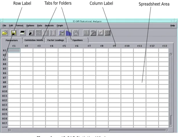
Figure 1 IC-CAP Statistics Window
Tabs for Folders Column Label Spreadsheet Area Row Label
1 From the File menu, choose Examples. The Examples Open dialog box appears.
2 Select bsim3.sdf from the list of files and choose OK.
3 The spreadsheet is loaded with data.
The spreadsheet displays the data in rows and columns. Each row contains one sample. Each column contains either a sample’s attribute, such as the sample ID, lot number, date, or temperature; or is a sample’s measured or extracted
data, such as VSAT, VTH0, or TOX. Attribute information is
displayed in blue, while parameter data is displayed in
N O T E
This BSIM3 data file is being used to teach you how to use the programonly. It does not contain validated data. Do not be concerned if you
Spreadsheet Format
The data may contain too many characters to fit in the cells. From the Format menu, choose Column Width, a dialog box appears. You enter a larger or smaller number in the field to fit your data. In this case, accept the default of 10 and choose OK.
Transform Data
One of the key assumptions made by multivariate techniques such as Factor Analysis is that the data set to be analyzed is a joint Gaussian distribution. If the data is not joint
Gaussian, then the model generated from the analysis may not accurately reproduce the measured density.
One of the ways to help convert a data set to Gaussian is to perform a mathematical transformation.
You have to decide which data columns need to be transformed. Some columns may already be Gaussian. As described below, you can quickly plot the data to see if it is
Gaussian. The next step, Eliminate Outlier Data, can be
done before the data transformation step, depending on the look of the data.
Selecting Columns and Rows
The spreadsheet columns have the labels C1, C2, C3, etc., just above the columns. The rows have the labels R1, R2, R3,
etc., just to the left of the rows. See Figure 1. To select an
entire column or row, move the cursor to the column or row label you want and press the left mouse button.
Plot and Analyze the Data
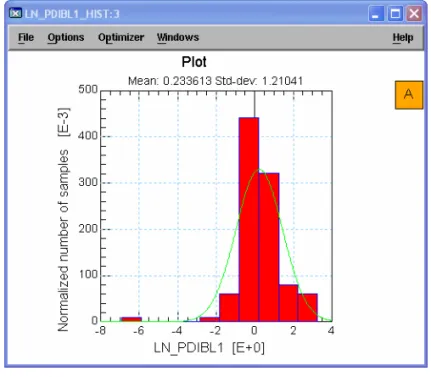
To view the data before transforming it, we will plot the data for column C8 as a histogram.
1 Select column C8 (parameter PDIBL1) by clicking column
label C8. The column is highlighted.
2 From the Graph menu choose Histogram (or click the
Histogram icon from the toolbar). A plot window appears with the histogram for that column.
When you are done viewing plots, you can choose File > Close from the Plot window.
Transform the Data
1 Select column C8 again.
2 From the Data menu, choose Data Transformations. A dialog
3 To select a transformation type, click the drop-down list button and select the type you want.
4 For this example, choose Natural Log and choose OK. The
data for column C8 is transformed.
The parameter name is appended with LN (for log natural) and becomes LN_PDIBL1.
Re-plot the histogram for column C8. Select column C8. From the Graph menu choose Histogram. Note that the data is now more Gaussian, but there is an outlier to the left.
Eliminate Outliers
There are several ways to eliminate outlier data or other invalid data. You can vary the order in which these methods are done. For example, you may immediately spot bad data and manually eliminate it, you can automatically filter the data to remove outliers, or you can plot the data in a histogram or scatter plot to help spot outliers. Often several iterations of these methods have to be performed until you’re satisfied that the data is ready for correlation analysis.
Plot and Analyze the Data
To help spot outlier data, let’s study the latest plot, above, for column C8. Note the that there appears to be an outlier at the far left of the plot, corresponding to a value of about -6.9. If you scan the data in the column, you will see that this value is in Figure 3 Histogram After Data Transform
Manually Eliminate Outliers
Let’s assume that from a review of the data, you believe the sample in row R20 is a bad sample.
1 To select this row, click row label R20.
2 From the Edit menu choose Deactivate. The row’s background
color changes to gray indicating that this sample is deactivated (to re-activate it, choose Edit > Activate).
3 Select column C8 again. From the Graph menu choose
Histogram. See that the plot is more Gaussian with the outlier eliminated.
Automatic Data Filtering
IC-CAP Statistics can automatically filter data based on minimum/maximum values or by a scale value. We will use a scale value. Scale is defined as the median absolute
deviation (MAD) divided by a constant (approximately 0.6745). This standardizes MAD in order to make the scale Figure 4 Histogram After Outlier Elimination
estimate consistent with the standard deviation of a normal distribution. The greater the scale value, the further from the median the filtering occurs.
1 Select column C8 again.
2 From the Data menu choose Data Filter. A dialog box is
displayed.
3 Accept the default Scale option (near top) to filter by a
scale value.
4 Change the Scale Limit (near bottom) to 4 by clicking the
right arrow or typing in the field. Then choose OK. The data is filtered based on this scale value. Note that eliminated rows are highlighted by a color change that indicates they have been filtered out. (The process can be undone by choosing Data > Undo Data Filtering.) Select column C8 once again. From the Graph menu choose Histogram. See that the plot is now more Gaussian with the data filtered.
Choose Statistical Summary for a Numeric Display
Besides a variety of plots to help you analyze your data, IC-CAP Statistics also has a Statistical Summary window (Analysis > Statistical Summary), which shows you standard statistical data, such as mean, variance, standard deviation, skewness, kurtosis, etc.
Repeat Data Transformation and Outlier Elimination for Other Columns
Repeat the steps outlined in the last two sections for each column that is non-Gaussian. For this example, you can skip this step.Perform Correlation Analysis
Correlation analysis provides a numerical measure of the amount of variation in one variable that is attributable to another variable. When an increase in the value of one variable Figure 5 Histogram After Data Filtering
is associated with an increase in the value of the other variable, the correlation is positive. When the increase is associated with a decrease, the correlation is negative.
Correlation analysis is always performed before proceeding to
factor analysis and the data used consists of all the rows in the
spreadsheet that have not been filtered, deactivated, or deleted.
To perform correlation analysis:
From the Analysis menu, choose Correlation Analysis. The Statistics window changes so that the Correlation Matrix folder is displayed. (If you want to go back to the parameter data before correlation analysis was performed, choose the folder tab labeled Parameters.)
The Correlation Matrix displays the same parameters down the rows and across the columns. The correlation coefficients for any two parameters are displayed where the rows and columns intersect. In the above example, the cell formed by R4 and C2 has a value of about 0.69, which shows moderate to strong correlation between parameters TOX and VTH0.
Perform Factor Analysis
Now that the correlation matrix is defined, the next step is to perform factor analysis.
1 From the Analysis menu, choose Factor Analysis, a dialog box
is displayed.
You choose the method of factor analysis from three choices: Principal Component, Principal Factor, or Unweighted Least Squares.
The Principal Component and Principal Factor methods, while quite different in assumptions, are similar in the end effect; the main difference lies in their respective error terms. Unweighted Least Squares is a method of factor analysis using an iterative process. A detailed description of
these methods can be found in Chapter 3, “Data Analysis.”
You choose a starting figure for the number of factors you want to be found in your analysis. After you see the results, which correspond to the percent variation that can be explained by this number of factors, you can increase or decrease the number and repeat the analysis.
3 In the Method field, choose the default Principal Component option button.
4 Accept the default Rotation Type of None.
5 Choose OK to perform the analysis. The screen changes to
display the Factor Loadings folder.
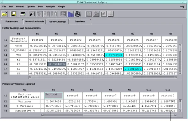
Two tables are generated in this window; the first contains the factor loadings. Factor loadings represent the
correlations between each factor and the model parameters. The second table presents a summary of the variances associated with each factor as well as a report of the percentage error explained by each factor.
Note that the cumulative percent for 10 factors, shown in the lower right cell, is about 82% (you may have to use the scroll bar to see it). This means that if only 10 factors were used to
make a statistical model from this data, the model would explain 82% of the variance compared to using all of the parameters/factors.
6 Now we will re-analyze using 14 factors. Choose Analysis >
Factor Analysis and enter 14 in the Number of Factors field. With 14 factors, the cumulative percent is about 92%, as shown in the lower right cell below. You have to decide how high a figure is acceptable for your work.
The top portion of the Factor Loading folder displays the data in a color-coded format. Factor Group data, one group per row, is displayed in a red font. Dominant Parameter data, one dominant parameter per column, is displayed with a blue background. A detailed description of both can be found in
“Perform Factor Analysis” on page 58.
Generate Equations
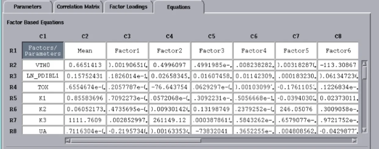
Next, we will generate equations from the factor analysis. You can generate equations from factors or dominant parameters. IC-CAP Statistics computes the equation coefficients that you use to build your SPICE model.
From the Analysis menu choose Generate Equations. A submenu with two choices appears to the right. Choose Factors. The screen changes to display the Equations folder
Cumulative % with 14 factors
.
Generate a Parametric Model
Now that the equation coefficients are generated, you can build a variety of statistical models, or save the data in a SPICE equations format for use in circuit simulations. You can choose from Monte Carlo, Corner, or Parametric Boundary models. You can test your model, based on a reduced set of parameters, against the raw data to see how well it performs. At this point, IC-CAP Statistics has been designed for flexibility to work with your process.
For our example, we will perform Monte Carlo analysis and compare the results to the raw data.
Perform Monte Carlo Analysis, Plot Data, and Compare
1 From the Analysis menu choose Parametric Analysis. A
submenu is displayed to the right. Choose Factor Equations, a dialog box is displayed.
2 Choose the Monte Carlo method.
3 In the Number of Outcomes field, enter 500 and choose OK.
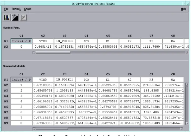
The results of the Monte Carlo analysis are displayed in the Parametric Analysis Results window. The number of rows is equal to the number of Monte Carlo outcomes, and the columns correspond to the parameters.
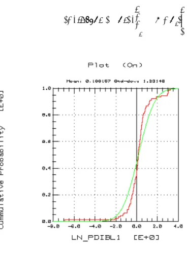
Earlier we used parameter PDIBL1 to plot as a histogram, and transformed the data to a more Gaussian fit, see
Figure 5.
4 Now, select the column for parameter PDIBL1 (now labeled
LN_PDIBL1 because we did a log transform of the data) in the Parametric Analysis Results window.
5 From the Graph menu choose Histogram.
6 Compare this plot (made from synthesized Monte Carlo data)
with the earlier plot.
Details on Corner Models and Boundary Models are found in
“Generate a Parametric Model” on page 64. Figure 6 Parametric Analysis Results Window
Non-Parametric Boundary Modeling
IC-CAP Statistics contains proprietary Agilent EEsof non-parametric analysis algorithms for identifying nominal models and worst-case-candidate models from arbitrary joint probability densities. This advanced feature, called
Non-Parametric Boundary Modeling, differs from the
parametric (joint Gaussian) methods described earlier, and can be used when the data is bimodal or otherwise non-Gaussian. Details on Non-Parametric Boundary Modeling are found in
2
Program Basics
Starting IC-CAP Statistics 32
Spreadsheet Format 34
Opening or Creating a File 37
Saving Data 43
Exporting Data 44
Printing 44
Closing and Exiting 44
Graphing Data 45
Using the Edit Menu Commands 49
Using the Format Menu Commands 51
Building a Parametric Model 52
Building a Non-Parametric Model 74
Other Analysis Menu Options 82
Chapter 1 introduced IC-CAP Statistics and used an example BSIM3 model file tutorial to show you how the program is typically used. If you haven’t already read Chapter 1, you should do so before continuing. In this chapter we will show you how to use most of IC-CAP Statistics’ basic functions.
Starting IC-CAP Statistics
To start the Statistics tool:
From the Main window, choose Tools > Statistics (or click the Statistics icon).
The Statistics window is displayed.
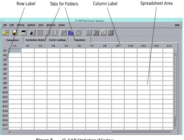
Figure 7 IC-CAP Statistics Window
Tabs for Folders Column Label Spreadsheet Area Row Label
Spreadsheet Format
The Main IC-CAP Statistics window appears in a spreadsheet format. The spreadsheet displays the data in rows and columns. Each row contains one sample. Each column contains either a sample’s attribute, such as the sample ID, lot number, date, or temperature; or is a sample’s measured or extracted data (parameters), such as Vsat, Voff, or DL. Attribute information is displayed in blue, while parameter data is displayed in black.
Changing Row Height or Column Width
Your data may contain too many characters to fit in the cells, or you may want narrower columns. The Format menu lets you change the number of characters for either rows or columns. Choose Row Height or Column Width, a dialog box appears. You enter a larger or smaller number in the field to fit your data. For columns, the number specifies the width in characters. This
action changes the size of all the rows or columns.
If you want to change only one column or row, position the
cursor along the cell edge line. The I-beam cursor turns into a pointer. Drag the pointer left or right to change columns, or up or down to change rows.
Selecting Rows and Columns
The spreadsheet columns have the labels C1, C2, C3, etc., just above the columns. The rows have the labels R1, R2, R3, etc., just to the left of the rows. To select an entire column or row, move the cursor to the column or row label you want and press the left mouse button.
N O T E
If you manually change row height or column width by dragging the celledge, those rows or columns cannot be altered with the Format menu command again during this Statistics session.
Selecting Multiple Rows or Columns
You may want to delete, deactivate, or activate multiple rows (containing your samples) or columns (containing your parameters).
• To select two or more rows or columns, select the first row or
column, then hold down the Control key before you select the next row(s) or column(s).
• To select all the rows or columns between two points, select
the first row or column, then hold down the Shift key before you select the last row or column. Or you can select the first row or column and drag the mouse over the rest of the desired rows or columns. The two rows or columns you selected and all those in-between are selected.
Folders
As shown in Figure 7, the Spreadsheet has tabs for four folders
that contain data for:
• Parameters. This folder contains your raw data (measured or
extracted), showing the parameters for each sample.
• Correlation Matrix. This folder shows how each parameter
correlates with every other parameter.
• Factor Loading. This folder displays the loadings
(correlations) that relate each model parameter to each of the derived factors as well as other data.
• Equations. This folder shows the equation coefficients
derived from the factor analysis that you use to build your SPICE model.
Click the tab to display the data for each of these areas. A full description of each of these areas is found later in this chapter.
Icons
Near the top of the Statistics Window there is a toolbar with a group of icons. These icons provide one-click access to
frequently used commands. Move the cursor just under each icon and leave it for a few seconds. A icon label appears that tells its function.
Save Print Clear Delete Open Activate Deactivate Correlation Factor Histogram Cumulative Plot Scatter Plot Data Transform
Opening or Creating a File
There are four ways to begin working with IC-CAP Statistics:
• Importing an ASCII text file containing your data
• Loading extraction data directly from IC-CAP
• Opening a file already in the IC-CAP Statistics data file (.sdf)
format, which is based on the MDIF file format
• Manually typing the data in the Statistics spreadsheet
Importing ASCII Data
One way to begin work with IC-CAP Statistics is to import ASCII data saved in another program, such as Lotus 1-2-3 or Microsoft Excel. The data must be delimited with spaces or tabs (not commas). To import the data:
1 Choose File > Import, a dialog box is displayed. Select the path
and name of the file you want to import and choose OK. The data is loaded into the spreadsheet. Complete details on
using this type of dialog box are found in “Working with
Dialog Boxes" in the User’s Guide.
2 You have to specify which columns are attributes and which
are parameters. The attribute columns have to be contiguous and on the left side of the spreadsheet. To specify that a column contains attributes, first select the columns. Then, choose Edit > Parameter to Attribute. If that column is not already at the left, it moves to the left and becomes an attribute column, denoted by a blue text font.
3 Repeat Step 2 for additional attribute columns. You can do
this for multiple columns at one time by holding down the Shift or Ctrl key while selecting columns.
4 You can reverse this process if necessary by choosing Edit >
Attribute to Parameter.
Loading Data from IC-CAP
There are two ways to load extracted model data from the Main IC-CAP program into Statistics:
• Using the supplied macro
• Manually executing PEL commands
The first method is preferable if you want automated file loading along with automated measurement and extraction. If you use the manual method, the IC-CAP Statistics window must be opened.
These procedures use IC-CAP’s Parameter Extraction Language
(PEL). For more information about PEL see Chapter 9,
“Parameter Extraction Language,” in the Reference manual.
Using the Supplied Macro
You will load the model file called load_stat_data.mdl, which
contains macro files. This file is shipped with the software and found in the Examples area.
The macro called Main loads parameters from a collection of
.mdl files into the Statistics Parameters spreadsheet. (The
macro called Load_Data is invoked by Main and you should not
use it.) Once the appropriate model variables have been set and
the .mdl parameter files have been created, the Main macro is
ready to be run. The macro is general, and can be run with any collection of .mdl files. To let you see how the macro works, a collection of example .mdl files are provided in the examples directory. The parameter values are automatically written to the Statistics Parameters spreadsheet through successive calls
to the PEL function icstat_from_partable.
Before you use the macro, do the following:
1 In order to use the macro, your model files must be in the
following format:
<base filename>_<n>.mdl
where n is an integer equal or greater than 1, and the first
model file must start with 1. For example, bsim_1.mdl
eebjt_1.mdl eebjt_2.mdl eebjt_3.mdl, etc.
2 All the model files must reside in the same directory. You will
indicate the pathname and the number of model files using model variables.
3 If you want attribute information to be automatically
transferred from the .mdl files, then the attribute values and labels (attribute parameter names) will have to be stored in variable arrays in the .mdl files. The attribute labels should be stored in an ICCAP_ARRAY called ATTRIBUTE_LABELS. The attribute values should be stored in an ICCAP_ARRAY called ATTRIBUTE_VALS. The size of the arrays is arbitrary, but you must explicitly specify it in the variable
NUM_ATTRIBUTES.
Now you are ready to use the macro.
1 From the Main IC-CAP program choose File > Examples. The
Examples Open dialog box appears.
2 Select the /statistics/load_data directory and then the
load_stat_data.mdl file from the list of files and choose OK. The model file loads.
3 Choose the Model Variables tab. A table appears with four
items. Ignore the first item (called Local_VAR). Enter data for the three remaining items, as follows:
4 Choose the Macros tab and select Main in the Select Macro
field.
5 Click the Execute button (left). The Statistics Parameters
spreadsheet is filled with data.
Name Value
numFiles Enter the total number of model files you want to load into Statistics
filesDirPath Enter the path to the directory that contains the model files
baseFileName Enter the base filename for your model files, such as bsim or
The following shows the macro.
N O T E
Your data may contain parameter columns (such as nominal temperature)that contain constants. You should deactivate these columns before performing correlation analysis.
! Open the statistics window dummy = icstat_open()
! Prompt the user on whether he is using the example data or his own data
LINPUT “Use the example .mdl files (y/n)?”,”y”,selection
if selection == “y” then
iccap_root=SYSTEM$(“echo $ICCAP_ROOT”)
filesDirPath=VAL$(iccap_root) & “/examples/model_files/statistics/load_data/” endif
! Prepend the path onto the file name and append _1.mdl to get the first ! file in the directory (all we care about is the parameter names, so any ! file in the directory would do).
filename = val$(filesDirPath) & val$(baseFileName) & “_1.mdl”
! Open the first file to get the parameter names menu_func(“/”, “Add Model”, “temp”)
menu_func(“/temp”, “Open”, filename)
! Load the parameter names into the first row
dummy = icstat_set_param_column_labels(“/temp”,”MODEL PARAMETERS”)
! Compute the number of rows in the empty spreadsheet and then insert enough ! additional rows so that the total number of rows = numFiles+1.
numRows = icstat_num_rows(“PARAMETERS”) if numRows < numFiles then
numInsert = numFiles - numRows
dummy = icstat_insert(numRows+1, numInsert, “ROW”) endif
! Load the data into the statistics spreadsheet using the “Load_Data” macro
menu_func(“/load_stat_macro/Load_Data”, “Execute”)
! Use the value of the variable NUM_ATTRIBUTES to insert enough columns at ! the beginning of the parameters spreadsheet to store the attributes.
Manually Executing PEL Commands
The following manual procedure is recommended only for transferring one or two rows of data to Statistics.
1 Open the IC-CAP model file from which you want to load
data into IC-CAP Statistics.
2 Open the Setup from the DUT-Setups folder.
3 Choose the Extract/Optimize folder from the setup.
4 Choose the Browse button (far right). The Function Browser
dialog box appears.
5 From the Function Groups field (left side), scroll down and
select Statistical Analysis.
dummy = icstat_insert(1, /temp/NUM_ATTRIBUTES, “COLUMN”)
! Write the attribute names to the first row of the spreadsheet ! and convert these column to attribute columns.
index=1
while index <= /temp/NUM_ATTRIBUTES
name = val$(/temp/ATTRIBUTE_LABELS[index-1]) dummy = icstat_set_text_cell(1, index, name) dummy = icstat_parameter_2_attribute(index) index=index+1
end while
! Cycle through the .mdl files and read the attributes and parameters into ! the parameters spreadsheet
i=1
while i <= numFiles
fileName = val$(filesDirPath) & val$(baseFileName) & “_” & val$(i) & “.mdl” print fileName
menu_func(“/temp”, “Open”, fileName) k=i+1
dummy = icstat_from_partable(k, “/temp”, “MODEL PARAMETERS”) index=1
! Here is the loop to set the attribute values while index <= /temp/NUM_ATTRIBUTES
value = val$(/temp/ATTRIBUTE_VALS[index-1]) dummy = icstat_set_text_cell(k, index, value) index=index+1
end while i=i+1 end while
6 Then select icstat_from_partable from the functions listed on the right side. Documentation on how to use the function (such as the arguments) is listed in the middle part of the dialog box. Choose the Select button at bottom. The Transform window is displayed again.
7 Fill in the arguments needed to complete the function. Then
choose Execute. The data from either the model or DUT parameter will appear in the Statistics Parameters spreadsheet.
8 Repeat this procedure for each additional row of data you
want send.
Opening a File in IC-CAP Statistics Format
To open a file already saved in the IC-CAP Statistics format, choose File > Open. The File Open dialog box appears. Enter the path and filename you want or select the file. IC-CAP Statistics
files use the .sdf extension.
IC-CAP Statistics is shipped with several example .sdf files. To open an example file, choose File > Examples. The Examples Open dialog box appears. Select the example file you want.
Manually Entering Data
Although this method would not typically be used, data can be entered (or modified) directly in the spreadsheet, attribute rows
can be defined (see “Importing ASCII Data” on page 37, step
2) and the file saved. To manually enter data in a new file, choose File > New.
N O T E
Before transferring any data, use the icstat_set_param_column_labelsSaving Data
To save data:
Choose File > Save As, the Save As dialog box is displayed.
You can save portions of your file, such as only the parameters and correlation matrix, or all of the elements in your file. Select the check box next to the parts of your file you want to save. The default is set to save all portions.
If you want to keep the present file and save your data under a new filename, enter a new filename in the Filename field at bottom.
Exporting Data
To export a file, choose File > Export. A submenu is displayed. Choose the format you want. There are three file formats that you can export from IC-CAP Statistics:
• Text File. Exports the data currently contained in the
Parameters folder (the raw data) in a row/column, space delimited (no commas or tabs) ASCII text format for use in other programs. If you choose this option, a dialog box is displayed. Enter a filename for the export file.
• SPICE Library File. Converts the data for desired samples
into a form usable as a SPICE library. If you choose this option, a dialog box is displayed. Enter a filename for the export file.
• SPICE Equations. Converts the data contained in the two
tables in the Equation folder into a form usable in a SPICE netlist. If you choose this option, a dialog box is displayed. You fill in the model file name, the sample row numbers you want to be saved, and a filename for the export file.
See Appendix A, “File Formats” for complete details on the structure of these file formats.
Printing
To print the contents of the current window or plot, choose File > Print, or click the Print icon. Choose File > Print Set to choose or alter printer setup parameters.
Closing and Exiting
Choose File > Close to close the file currently opened without leaving IC-CAP Statistics. Choose File > Exit Statistics to exit IC-CAP Statistics and return to the Main IC-CAP window.
Graphing Data
After you load the raw data, you may want to plot the data for a given parameter in one or more formats. Or, you may want to re-plot the data after performing a mathematical
transformation or manipulation. To create a graph, choose Graph and then the type of plot you want (such as Histogram). IC-CAP Statistics contains the following type of plots:
IC-CAP’s Statistic Analysis Histogram is normalized. The definition of the histogram normalization is as follows: Assume:
Variable X indicated the width of the histogram bin,
Variable n indicated the number of the histogram bins.
Variable Yiindicated the number of samples for the
histogram bin with index of i
Variable normalize_Yiindicated the normalized number of
samples for the histogram bin with index of i
Then we have,
Figure 9 Cumulative Density Plot
normalize_Yi ( )Yi (X×Yi) i–1 n
∑
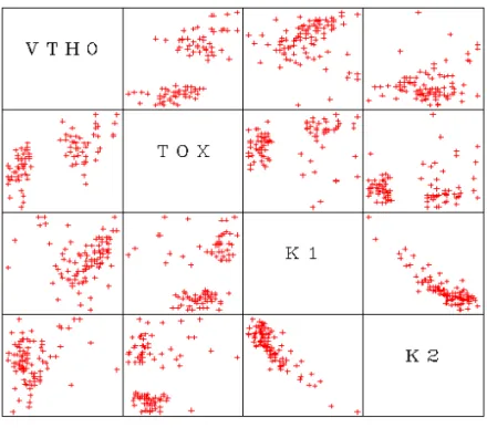
⁄ =The scatter plot matrix contains multiple scatter plots, with each parameter plotted against every other parameter. For example, if your data had four parameters, P1, P2, P3, and P4, the matrix would contain 16 cells. First would be P1 against itself (only the label appears), then P1 vs. P2, P1 vs. P3, and then P1 vs. P4. The next row would contain P2 vs. P1, the P2 label, P2 vs. P3, and P2 vs. P4, and so on. If you have a large number of parameters, the plots will be quite small. Select the columns you want to plot and choose Graph > Scatter Plot Matrix. More information on of each of these plots can be found in
Chapter 4, “Data Visualization.” Figure 11 Scatter Plot Matrix
Using the Edit Menu Commands
Refer to the table below for a list of features and functions found on the Edit menu.
Command Function Use
Swap Reverses the order of any 2 rows or columns
Choose Row or Column. Enter the row or column number you want to swap from in the From field. Enter the row or column number where you want it to go in the To field. The two rows or columns will be exchanged.
Move Moves one or more rows or columns to another place in the table
Choose Row or Column. Enter the row or column number you want to move from in the From field. Enter the row or column number where you want it to be moved to in the To field. The moved row(s) or column(s) will be inserted in the table.
Copy Copies one or more rows or columns to another place in the table
Choose Row or Column. Enter the row or column number you want to copy from in the From field. Enter the number where you want it to go in the To field. The copied row(s) or column(s) will replace the data in one or more row(s) or column(s), as selected.
Insert Inserts one or more rows or columns
Choose Row or Column. Select the row or column you want to insert more rows or columns before. Enter the number of rows or columns you want to insert.
Sort Sorts the data in a column
Select the column in which you want to sort data. Choose Ascending or Descending. You can’t sort row data.
Clear Deletes the data but leaves the row or column
Select a row or column. Choose Clear and the data is erased.
Delete Deletes the data along with the row or column
Select a row or column. Choose Delete and the row or column is removed from the table.
Activate Activates a row or column that has been deactivated
Select a row or column. Choose Activate to reactivate a row or column that has been deactivated. A deactivated row’s or column’s background color is gray.
Deactivate Deactivates a row or column
Select a row or column. Choose Deactivate to deactivate a row or column. The row’s or column’s background color changes to gray. You can deactivate a row to eliminate an outlier sample or for other reasons. Flip Active
to Deactive
Activates rows (or columns) which are not active; deactivates rows (or columns) which are active
The Flip feature is provided to make it easier to reach the desired goal when more than half of the rows or columns need to have their active status reversed. In this case, just change the ones that are correct to the other status, and then Flip all the rows (or columns) at once.
Hide Attributes
Controls whether or not the Attribute columns are visible in the table
This functions as a toggle. When the Attribute columns are hidden, an option marker appears next to this menu item. Use this feature to view only the parameters. Attribute
to Parameter
Tells the program to change a column from Attribute to Parameter
Select a row or column. Choose Attribute to Parameter to change a column from an Attribute column to a Parameter column.
Parameter to Attribute
Tells the program to change a column from Parameter to Attribute
Select a row or column. Choose Parameter to Attribute to change a column from a Parameter column to an Attribute column.
Command Function Use
N O T E
Several of the Edit menu functions have toolbar icons. See “Icons” onUsing the Format Menu Commands
Refer to the table below for a list of features and functions found on the Format menu.
Command Function Use
Row Height
Allows you to change the row height
Enter a number to increase or decrease the height of all rows. The number corresponds to the height of a row.
Column Width
Allows you to change the column width
Enter a number to increase or decrease the width of all columns. The number corresponds to the number of characters in a column. Color Allows you to
change the color settings for the spreadsheet
You can select colors for seven areas: Table Background, Table Foreground, Selection Background, Deactivate, Parameter Attribute, Data Filter, and Attribute Filter. To change colors, click on the down arrow.
Building a Parametric Model
In Chapter 1 we went through the typical steps needed to take raw extraction data and develop a parametric statistical model. This exercise was done as a tutorial on IC-CAP Statistics. If you haven’t read this section, please refer to the procedure, which
begins with “Transform Data” on page 15. In this chapter,
we will provide expanded information on some of the steps related to building a statistical model.
The general steps needed to build a parametric statistical model are:
1 Measure and extract model parameters
2 Start IC-CAP Statistics and import data
3 Transform distributions to Gaussian
4 Eliminate outlier data
5 Perform correlation analysis
6 Perform factor or principal component analysis
7 Generate model equations
8 Generate models
9 Test models
Transforming Distributions/Eliminating Outliers
As stated in Chapter 1, one of the key assumptions made by multivariate techniques such as Factor Analysis is that the data set to be analyzed is a joint Gaussian distribution. If the data is not joint Gaussian, the model generated from the analysis may not accurately reproduce the measured density.
Therefore steps 3 and 4 in our procedure to build a statistical model can be done in any order. The elimination of outlier data can be done before or after data transformation. Outliers can be eliminated manually or through automatic data filtering.
Data Transformation
You have to decide which data columns need to be transformed. Generally, only some of the columns contain key parameters. Some columns may already be Gaussian. You can quickly plot the data to see if it is Gaussian.
To transform data, select a column and then choose Data > Data Transformations, a dialog box appears with the mathematical transforms available, as shown in the table below. To show the transformation, in some cases the parameter name is appended, also as shown in the table. For example, parameter TOX would become LN_TOX in a natural log transform.
Transformation Label Appended to Name
None Exponential EXP Natural Log LN Square Root SQRT Square SQR Constant Value Mean
To select a transformation type, click the drop-down list button and select the type you want. If you select Constant Value, the Value field (center) becomes active, and you can enter the constant you want to substitute for your data.
Pairs of the transforms work as opposites. If you transform your data using Natural Log and want to undo the change, choose Exponential. Similarly, Square and Square Root work the same way. To undo either Constant Value or Mean, however, choose Undo Constant/Mean. More complex transformation types are available in the Main IC-CAP program. You can export data to be transformed and then import it back into Statistics.
Manually Eliminating Outliers
You can manually eliminate outliers by deactivating any row you believe contains outlier data. Select the row that contains the sample you want to deactivate and choose Edit > Deactivate or click the icon on the toolbar.
Automatic Data Filtering
You can automatically filter your data to eliminate outliers. IC-CAP Statistics can filter data based on minimum/maximum values or by a scale value. Scale is defined as the median absolute deviation (MAD) divided by a constant (approximately 0.6745). This standardizes MAD in order to make the scale estimate consistent with the standard deviation of a normal distribution. The greater the scale value, the further from the median the filtering occurs. If too much data is eliminated using, for example, a scale value of 4, you can retrieve some of the data by repeating a single-pass filtering operation with a scale value of 3.
To use the Data Filter feature:
1 Select a column you want to filter.
3 To filter by a scale value, choose the Scale option button. Change the Scale Limit (near bottom) to the number you want by clicking the right arrow or typing in the field.
4 To filter by minimum/maximum values, choose the
Minimum/Maximum option button and then enter your minimum and maximum values in the lower portion of the dialog box.
5 The Filter Type field (center) allows you to filter samples by a
single pass or cumulatively. Choosing Cumulative means that rows eliminated during one filter pass remain deactivated during the subsequent filtering passes, regardless of the filtering criteria of the subsequent passes. Single Pass filtering deactivates rows based on only one filtering operation.
6 When done, choose OK.
The data is filtered based on the parameters you chose. Note that eliminated rows are highlighted by a color change that indicates they have been deactivated.
Repeat Data Transformation and Outlier Elimination for Other
Columns
Repeat the above steps for each column of data you want to make Gaussian through data transformation, manual outlier elimination, or data filtering.
Attribute Filter Options
Besides Data Filter and Undo Data Filtering, there are the companion choices of Attribute Filter and Undo Attribute Filtering. These choices work in the same manner as parameter data filtering but apply only to attribute columns.
To use the Attribute Filter feature:
1 Select an attribute column you want to filter.
2 Choose Data > Attribute Filter. A dialog box is displayed.
3 If you want to filter by a character string that matches an
attribute label (such as “sample1”), choose Text in the Filter By field, and enter the text in the Text to match field.
4 If you want to filter by a range of values (such as sample23 to
sample29), choose Range in the Filter By field and enter the minimum and maximum values in the right-center part of the box.
5 The Filter Type field allows you to filter samples by a single
criteria of the subsequent passes. Single Pass filtering deactivates rows based on only one filtering operation.
6 When done, choose OK.
Performing Correlation Analysis
As stated in Chapter 1, correlation analysis provides a numerical measure of the amount of variation in one variable that is attributable to another variable. When an increase in the value of a variable is associated with an increase in the value of the other variable, the correlation is positive. When the increase is associated with a decrease the correlation is negative.
Correlation analysis is always performed before proceeding to factor analysis and the data used consists of all the rows in the spreadsheet that have not been filtered, deactivated, or deleted. To perform correlation analysis, choose Analysis > Correlation Analysis. The Statistics window changes so that the Correlation Matrix folder is displayed. (If you want to go back to the parameter data before correlation analysis was performed, choose the folder tab labeled Parameters.)
The Correlation Matrix displays the same parameters down the rows and across the columns. The correlation coefficients for any two parameters are displayed where the rows and columns intersect. In the preceding example, the cell R4 C2 has a value of about 0.69, which shows moderate to strong correlation
between parameters TOX and VTH0.
Perform Factor Analysis
Now that the correlation matrix is defined, the next step is to perform factor analysis. To perform factor analysis, choose Analysis > Factor Analysis, a dialog box is displayed.
You choose the method of factor analysis from three choices:
• Principal Component —The principal component model of
factor analysis. Direct calculation; no iterations.
• Principal Factor—Principal factor analysis. Direct
calculation; no iterations.
• Unweighted Least Squares—A method of factor analysis using
an iterative process. This methods is also knows as minres or the minimum residual method.
principal component method, without factor rotation, is preferred. If factor analysis is being used as an interim step in building a regression model, then principal factor analysis or unweighted least squares should be used with one of the three rotation types.
A detailed description of each of these three methods can be
found in Chapter 3, “Data Analysis.”
You choose a starting figure for the Number of Factors you want to be found in your analysis. After you see the results, which correspond to the percent variation that can be explained by this number of factors, you can increase or decrease the number and repeat the analysis.
The Rotation Type field has four choices.
• Varimax
• Quartimax
• Equimax
• None (default)
For more information on factor rotation, refer to “Factor
Rotation” on page 98.
The Iteration Control button (upper right) controls fine tuning for the Unweighted Least Squares and Rotation functions.
Therefore, if you select the Unweighted Least Squares method and click Iteration Control, a dialog box is displayed. You accept the default values (as shown) or choose User and type in the values for the following four parameters, as desired:
• Maximum Iteration. The maximum number of iterations that
will be attempted before arriving at a solution.
• Convergence - Iterations. When the relative change in the
criterion function is less than this number from one iteration to the next, convergence is assumed.
• Maximum Steps. The maximum number of step halvings
allowed during any one iteration.
• Convergence - 2nd Derivative. When the largest relative
change in the unique standard deviation vector is less than this number, exact 2nd derivatives are used.
Likewise, if you select a rotation type other than None in the Factor Analysis dialog box, and click Iteration Control, the same
• Maximum Iterations. The maximum number of iterations that will be attempted before arriving at a solution.
• Convergence. When the relative change in the criterion
function is less than this number from one iteration to the next, convergence is assumed.
When done, choose OK to return to the Factor Analysis dialog box and OK again perform the factor analysis. The screen changes to display or update the Factor Loadings folder.
Factor Loadings Folder
Two tables are generated in the Factor Loadings folder. The first table contains the factor loadings, which represent the loadings (correlations) that relate each model parameter to each of the derived factors. This table also has a column called
Figure 12 Factor Analysis Folder
Communality, always displayed at the far right part of the table. This field shows the variance explained by all of the factors for a single parameter.
The top portion of the Factor Loading folder displays the data in a color-coded format. Factor Group data, one group per row, is displayed in a red font. Dominant Parameter data, one dominant parameter per column, is displayed with a blue background. These terms are defined as follows:
Factor Group. The factor group shows, for a given parameter, which factor the parameter is most highly correlated with. Dominant Parameter. The dominant parameter is the one parameter in the column that has the highest loading (correlation).
The second table has three fields:
• Variance. Presents a summary of the variances associated
with each factor. For example, a variance of 3.45 indicates that the factor accounts for as much variance in the data collection as would 3.45 variables, on average.
• % Variance. Shows how much of the variance of all the
parameters is explained by a single factor.
• Cumulative %. Shows how much of the variance of all the
parameters is explained cumulatively by from one to all of the factors. That is, as you move left to right in the table, the percentage increases as more and more factors are included. Note that the cumulative percent for the example shown in
Figure 12, which was analyzed for 10 factors, is about 82%. See the lower right cell in the figure. This means that if only 10 factors were used to make a statistical model from this data, the model would explain 82% of the variance compared to using all of the parameters/factors.
With 14 factors, the cumulative percent is about 92%, as shown in the lower right cell below. You have to decide how high a figure is acceptable for your work.
Factor Loadings Options on the Analysis Menu
The last four options on the Analysis menu are specifically for the Factor Loadings folder, and are only active when there is factor analysis data present. The options are as follows:
• Change Dominant Parameter. Select a cell that you want to
become the dominant parameter for that column and then choose Analysis > Change Dominant Parameter. The program replaces the calculated dominant parameter with the one you chose. To revert back to the calculated dominant parameter, choose Analysis > Default Dominant/Grouping.
• Change Factor Group. Select a cell that you want to become
the factor group for that parameter and then choose Analysis > Change Factor Group. The program replaces the calculated factor group with the one you chose. To revert back to the calculated factor group, choose Analysis > Default
Dominant/Grouping.
• Default Dominant/Grouping. If you changed either the
dominant parameter or the factor group, and you want to revert back to the one calculated by the program, choose Analysis > Default Dominant/Grouping.
• Factor/Parameter Groups. Choose Analysis > Factor/Parameter
Groups to display a summary table, which shows the
dominant parameter for each factor and its value, as well as the factor group data. The dominant parameter data is shown first. For a given factor, all parameters that belong to that group are shown.
Cumulative % with 14 factors
Generate Equations
The next step is to generate equations from the factor analysis. IC-CAP Statistics supplies the equation coefficients that you use to build your SPICE model.
To generate equations, choose Analysis > Generate Equations. A submenu with the two choices by which the equations will be generated appears to the right. Choose either Factors or Dominant Parameters. The screen changes to display the Equations folder, which, has two tables. The upper table displays factor based equations, the lower table displays dominant parameter based equations.
Generate a Parametric Model
Now that the equation coefficients are generated, you can build a variety of statistical models, or save the data in a SPICE equations format for use in circuit simulations. You can test your model, based on a reduced set of parameters, against the raw data to see how well it performs. At this point, IC-CAP Statistics has been designed for flexibility to work with your process.
• Regression Equations (see “Parametric Analysis Results Window” on page 66)
Factor Equations
To build the parametric model from factor equations, choose Analysis > Parametric Analysis > Factor Equations, a dialog box appears with three choices:
• Monte Carlo
• Corner
• Parametric Boundary
The advantages and disadvantages of these methods is
described beginning with “Parametric Analysis Results
Window” on page 66.
If you select Monte Carlo, you fill in the number of outcomes you want in the field below. If you select Corner or Parametric Boundary, you fill in the number of +/- sigmas you want. When done, choose OK. The Parametric Analysis Results window is displayed.
Parametric Analysis Results Window
When you perform a parametric analysis, the results are displayed in a window as shown in the previous figure. The upper spreadsheet displays the nominal point of a corner or parametric boundary analysis. The lower spreadsheet contains the rows for the samples (or Monte Carlo outcomes) and columns for the parameters. This window also has menu functions similar to those available in the Parameters folder, and include:
• File menu. Save As, Export, Print, and Close. For more
information, refer to “Saving Data” on page 43, “Exporting
Data” on page 44, “Printing” on page 44, and “Closing and Exiting” on page 44.