Vol 4, No 11 (2013)

Available online throug

ISSN 2229 – 5046

NUMERICAL SOLUTION FOR HYBRID FUZZY SYSTEMS BY SINGLE TERM HAAR

WAVELET SERIES TECHNIQUE

S. Sekar*

Department of Mathematics, Government Arts College (Autonomous),

Salem - 636 007, Tamil Nadu, India.

S. Senthilkumar

Department of Mathematics, A.V.C. College (Autonomous), Mannampandal,

Mayiladuthurai – 609 305, Tamil Nadu, India.

(Received on: 19-10-13; Revised & Accepted on: 13-11-13)

ABSTRACT

T

his paper presents numerical solutions for hybrid fuzzy differential equations by an application of the single-term Haar wavelet series (STHWS) technique, fourth order Runge-Kutta Method and Runge-Kutta Fehlberg method to solve the hybrid fuzzy differential equations [6 - 7]. The discrete solutions obtained through STHWS technique are compared with that of the Improved Euler method. The applicability of the STHWS technique is more suitable to solve the hybrid fuzzy differential equations.

Mathematics Subject Classification: 41A45, 41A46, 41A58.

Keywords: Haar wavelet; single-term Haar wavelet series (STHWS), Fuzzy differential equations, Fuzzy sets,

Hybrid Fuzzy differential equations.

1. INTRODUCTION

Hybrid systems are devoted to modelling, design, and validation of interactive systems of computer programs and continuous systems. That is, control systems that are capable of controlling complex systems which have discrete event dynamics as well as continuous time dynamics can be modelled by hybrid system. The differential systems containing fuzzy valued functions and interaction with a discrete time controller are named hybrid fuzzy differential systems. For analytical results on stability properties and comparison theorems we refer reader to [10, 11, 14].

In this article we developed numerical methods for addressing hybrid fuzzy differential equations by an application of the STHW technique which was studied by S. Sekar and team of his researchers [15 - 21]. In section 2 we list some basic definitions for fuzzy valued functions. In Section 3 reviews hybrid fuzzy differential systems. In Section 4 contains the properties of Haar wavelets and STHWS technique for approaching hybrid fuzzy differential equations and a convergence theorem. In Section 5 contains a numerical example to illustrate the theorem. We refer [1, 2, 9, 12 - 13] for the numerical treatment of fuzzy differential equations.

2. PRELIMINARIES

Denote by

E

1the set of all functions u : R → [0, 1] such that (i) u is normal, that is, there exist an

x

₀

∈

R

such that

( )

x

₀

=

1

u

, (ii) u is a fuzzy convex, that is, for

x

,

y

∈

R

and 0 ≤ λ ≤ 1, u(λx + (1 −λ)y) ≥ min{u(x), u(y)}, (iii) u is upper semicontinuous, and (iv) [u]0≡ the closure of {x ∈R: u(x) > 0} is compact. For 0 < α≤ 1, we define [u]α ={x ∈R:u(x) ≥ α}. An example of a u ∈

E

1 is given by

( )

(

(

]

)

(

)











∉

∈

+

−

∈

−

=

.

5

.

1

,

75

.

0

,

0

,

5

.

1

,

1

,

3

2

,

1

,

75

.

0

,

3

4

x

if

x

if

x

x

if

x

x

u

(1)

Corresponding author: S. Sekar*

The α-level sets of u in (1) are given by

[u]α = [0.75 + 0.25α, 1.5 − 0.5α]. (2)

For later purpose, we define

0ˆ

∈

E

1 as

0ˆ

( )

x

=

1

if x = 0 and

0ˆ

( )

x

=

0

if

x

≠

0

.

Next we review the Seikkala derivative [22] of x: I →

E

1where I⊂ R is an interval. If

[x(t)

α

]

=

[x

α

(t),

x

α

(t)]

for all t∈ I and α ∈ [0, 1], then

[

x

′

(t)

α

]

=

[(

x

α

)

′

(t),

(

x

α

)

′

(t)]

if

x

′

( )

t

∈

E

1. Next consider the initial value problem (IVP)

( )

_{( )}

( )

(

( )

)







=

=

′

=

0

0

,

,

x

x

t

x

t

f

t

x

x

u

(3)

where f : [0,∞) × R → R is continuous. We would like to interpret (3) using the Seikkala derivative and

x

₀

∈

E

1.

Let

[x

0

]

[

x

0

,

x

0

]

α α α

₌

and

[x(t)

]

α

=

[

x

α

(t),

x

α

(t)]

. By the Zadeh extension principle we get f: [0, ∞) × 1

E

→

E

1 where



_

f t,x

( )

_

 =

α

_



min f t,u :

{

( )

u

∈

_



x (t), x (t)

α α

_



}

, max f t,u :

{

( )

u

∈

_



x (t), x (t)

α α



_{ }

}



.





Then x: [0, ∞) →

E

1 is a solution of (3) using the Seikkala derivative and

x

₀

∈

E

1if

( )

{

( )

[

]

}

( )

x

(t)

max

{

f

( )

t,

u

:

[

x

(t),

x

(t)

]

}

,

x

(0)

x

,

,

x

(0)

x

,

(t)

x

(t),

x

:

u

t,

f

min

(t)

x

0 0

α α

α α α

α α

α α α

=

∈

=

′

=

∈

=

′

u

u

,

for allt ∈ [0,∞) and α ∈ [0, 1]. Lastly consider an f : [0,∞) × R × R → R which is continuous and the IVP

( )

(

( )

)

( )







=

=

′

0

0

,

,

,

x

x

k

t

x

t

f

t

x

(4)

As in [3], to interpret (4) using the Seikkala derivative and x0, k ∈ 1

E

, by the Zadeh extension principle we use f : [0,∞) ×

E

1 ×

E

1 →

E

1 where

(

)

{

(

)

}

(

)

{

}

k k

k k

, ,

[min f t,u,u

:

x (t), x (t) , u

k , k

,

max f t,u,u

:

x (t), x (t) , u

k , k

]

f t x k

u

u

α _{α α α α}

α α α α











 =

∈

∈





















∈

_

_

∈

_

_

where

k

α

=

[

k

α

,

k

α

]

. Then x: [0, ∞) →

E

1 is a solution of (4) using the Seikkala derivative and x0, k ∈ 1

E

if

( )

{

(

)

[

]

[

]

}

( )

x

(t)

max

{

f

(

t,

u,

u

)

:

[

x

(t),

x

(t)

]

,

u

[

k

,

k

]

}

,

x

(0)

x

,

,

x

(0)

x

,

k

,

k

u

,

(t)

x

(t),

x

:

u

u,

t,

f

min

(t)

x

0 k

k

0 k

k

α α

α α α

α α

α α

α α α

α α

=

∈

∈

=

′

=

∈

∈

=

′

u

u

for all t ∈ [0,∞) and α ∈ [0, 1].

3. THE HYBRID FUZZY DIFFERENTIAL SYSTEM

Consider the hybrid fuzzy differential system

( )

(

( )

( )

)

[

]

( )

=

_





∈

=

′

₊

,

,

,

,

,

,

1

k t k

k k k

k

x

t

x

t

t

t

t

x

t

x

t

f

t

x

λ

(5)

where

x

′

denotes Seikkala differentiation, 0 ≤ t0 < t1 < ・・・ < tk < ・・・ , tk→∞,

( )

( )

(

( ) ( )

) ( )

( )

(

( ) ( )

) ( )

( )

(

( ) ( )

) ( )

















≤

≤

=

=

′

≤

≤

=

=

′

≤

≤

=

=

′

=

′

+

.

.

.

,

,

,

,

,

.

.

.

,

,

,

,

,

,

,

,

,

,

1 2 1 1 1 1 1 1 1 1 1 0 0 0 0 0 0 0 0 k k k k k k k k

k

t

f

t

x

t

x

x

t

x

t

t

t

x

t

t

t

x

t

x

x

t

x

t

f

t

x

t

t

t

x

t

x

x

t

x

t

f

t

x

t

x

λ

λ

λ

Assuming that the existence and uniqueness of solution of (5) hold for each [tk, tk+1], by the solution of (3) we mean

the following function:

( ) (

)

( )

( )

( )

















≤

≤

≤

≤

≤

≤

=

+

.

.

.

,

,

.

.

.

,

,

,

,

,

,

1 2 1 1 1 0 0 0 0 k k

k

t

t

t

t

x

t

t

t

t

x

t

t

t

t

x

x

t

t

x

t

x

We note that the solution of (5) are piecewise differentiable in each interval for t ∈ [tk, tk+1] for a fixed xk∈ 1

E

and k=0, 1, 2, . . .

Using a representation of fuzzy numbers studied by Goestschel and Woxman [4] and Wu and Ma [23], we may

represent x∈

E

1 by a pair of functions

(

x

( ) ( )

r

,

x

r

)

,

0 ≤ r ≤ 1, such that (i)

x

( )

r

,

is bounded, left continuous, and non decreasing, (ii)

x

( ),

r

is bounded, left continuous, and non increasing, and (iii)

x

( ) ( )

r

≤

x

r

,

0 ≤ r ≤ 1. For example, u ∈

E

1given in (1) is represented by

(

u

( ) ( )

r

,

u

r

)

= (0.75 + 0.25r, 1.5 − 0.5r), 0 ≤ r ≤ 1, which is similar to [u]α given by (2).

Therefore we may replace (5) by an equivalent system

( )

(

( )

)

( )

( )

( )

(

( )

)

( )

( )









=

≡

=

′

=

≡

=

′

,

,

,

,

,

,

,

,

,

,

,

,

k k k k k k k k k k

x

t

x

x

x

t

G

x

x

t

f

t

x

x

t

x

x

x

t

F

x

x

t

f

t

x

λ

λ

(6)

which possesses a unique solution

( )

x,

x

which is a fuzzy function. That is for each t, the pair

[

x

( ) ( )

t

;

r

,

x

t

;

r

]

is a fuzzy number, where

x

( ) ( )

t

;

r

,

x

t

;

r

are respectively the solutions of the parametric form given by

( )

(

( ) ( )

)

( )

( )

( )

(

( ) ( )

)

( )

( )









=

=

′

=

=

′

,

;

,

;

,

;

,

,

;

,

;

,

;

,

r

x

r

t

x

r

t

x

r

t

x

t

G

t

x

r

x

r

t

x

r

t

x

r

t

x

t

F

t

x

k k k k k k (7)

for r ∈ [0, 1].

4. PROPERTIES OF HAAR WAVELET AND STHW TECHNIQUE

4.1 HAAR WAVELET SERIES

The orthogonalset of Haar wavelets

h

_i

( )

t

is a group of square waves with magnitude of

±

1

in some intervals and zeros elsewhere. In general,

h

_n

( )

t

=

h

₁

(

2

j

t

−

k

)

,

Where

n

=

2

j

+

k

,

j

≥

0

,

0

≤

k

<

2

j

,

n

,

j

,

k

∈

Z

.

Any function y(t), which is square integrable in the interval [0, 1) can be expanded in a Haar series with an infinite number of terms

,

)

(

)

(

0

∑

∞ =

=

i i

i

h

t

c

t

where the Haar coefficients

j

≥

0

,

0

≤

k

<

2

j

,

t

∈

[

0

,

1

)

,

=

∫

( )

1

0

)

(

2

y

t

h

t

dt

c

_i j _i are determined such that the

following integral square error

ε

is minimized

∫

( )

∑

( )

_











₋

=

− = 1 0 2 1 0

,

dt

t

h

c

t

y

m i i i

ε

Where

m

=

2

j

,

j

∈

{ }

0

∪

N

Furthermore

,

,

0

2

0

,

0

,

2

,

2

2

)

(

)

(

1 0 1













≠

<

≤

≥

+

=

=

=

=

− −

∫

h

t

h

t

dt

_i

i

_l

l

k

j

k

j j

j

il j

i

δ

usually, the series expansion

Eq. (8) contains an infinite number of terms for a smooth y (t). If y (t) is a piecewise constant or may be approximated as a piecewise constant, then the sum in Eq. (8) will be terminated after m terms, that is

( ) ( )

[

)

1

0

( )

( )

( ),

0,1

m

T

i i m m

i

y t

c h t

_c

h

t

t

= =

≈

∑

=

∈

( )

( )

[

0 1

...

1

]

,

T m

m

t

c

c

c

c

=

₋

( )

[

( ) ( )

( )

]

T m

m

t

h

t

h

t

h

t

h

=

₀

,

₀

,...,

₋₁

where “T” indicates transposition, the subscript m in the parentheses denotes their dimensions,

C

_{( )}T_m

h

_(m)

(

t

)

denotes the truncated sum. Since the differentiation of Haar wavelets results in generalized functions, which in any case should be avoided, the integration of Haar wavelets are preferred.

Integration of Haar Wavelets should be expandable in Haar series

∫

∑

∞ =

=

t i i i

m

d

C

h

t

h

0 0

)

(

)

(

τ

τ

If we truncate to

n

m

=

2

terms and use the above vector notation, then integration is performed by matrix vector multiplication and expandable formula into Haar series with Haar coefficient matrix defined by Hsiao [5].

( )

( )

( ) ( )

[

)

1

0

( ),

0,1

m m m m

h

τ τ

d

≈

E

_×

h

t

t

∈

∫

where the m-square matrix E is called the operational matrix of integration which satisfies the following recursive equations ( )





















































−

=

    _× −     ×       ×     × × 2 2 1 2 2 2 2 2 2

0

2

1

2

1

m m m m m m m m m m

H

m

H

m

E

E

(9)

( )





















−

=

×

0

4

1

4

1

2

1

2 2

E

and _{( )}

2

1

1 1×

=

E

The

[

]

m

i

x

m

i

x

h

x

h

x

h

x

h

H

m m n n n m m i

1

,

)

(

)...,

(

).

(

),

(

0 1 2 1

+

≤

≤

=

₋ ×

( )

1

( )

(

),

1

r

dia

H

m

H

−_m×m



T_m×m











=

1,1, 2, 2, 4, 4, 4,...

,

,

...

,

2

2 2 2

2

T

n

m m m

m

r

m









=

_

_

>













Proof of equation (9) is found in [5]. Since

H

_(mxm)and

H

₍−_m1_×m)contain many zeros. Let us define

( )

( )

t

h

( )

(

t

)

M

( )

(

t

)

4.2 SINGLE TERM HAAR WAVELET SERIES TECHNIQUE

With the STHWS approach, in the first interval, the given function is expanded as STHWS in the normalized

interval

τ

∈

[

0

,

1

)

, which corresponds to











∈

m

1

,

0

τ

by defining

τ

=

mt

, m being any integer. In STHWS, the

matrix becomes

2

1

=

E

. Let

( )

•

τ

x

and

x

( )

τ

be expanded by STHWS in the first interval as

x

( )

τ

=

ν

( )1

h

_o

( )

τ

•

,

( )

_τ

( )

_{( )}

_τ

0 1

h

x

x

=

and in the nth interval as,

x

( )

τ

=

ν

( )n

h

_o

( )

τ

•

,

x

( )

τ

=

x

( )n

h

₀

( )

τ

Integrating (9) with

1

2

E

=

,

we get ( )1

1

( )1

( )

0 .

2

x

=

ν

+

x

Where

x

(0)

is the initial condition. According to [7], we have

( )1

_{( )}

_{( ) ( )}

₁

₀

x

x

d

x

=

−

=

_∫

•

τ

τ

ν

In general, for any interval n, n=1, 2...

We obtain, ( ) ( )

(

1

)

2

1

₊

₋

=

v

x

n

x

n n (10)

x

( )

n

=

v

( )n

+

x

(

n

−

1

)

(11) Equation (10) and (11) give the discrete time values of

x

( )n and

x

( )

n

x n

( )

for the nth interval. These values from the basis for the estimating block pulse values and discrete values in the subsequent normalized time intervals.

5. NUMERICAL EXAMPLE

Consider the following hybrid fuzzy IVP, [6 – 7]

( ) ( ) ( ) ( )

[

]

( ) (

[

) (

)

]

_





≤

≤

−

+

=

=

=

∈

+

=

′

₊

,

1

0

,

125

.

0

125

.

1

,

25

.

0

75

.

0

;

,...

3

,

2

,

1

,

0

,

,

,

,

₁

r

e

r

e

r

r

t

x

k

k

t

t

t

t

t

x

t

m

t

x

t

x

t t k k k k k

λ

(12)

where

( )

(

(

)

)

(

)

(

)

(

)

(

)







>

−

≤

=

5

.

0

1

mod

1

mod

1

2

5

.

0

1

mod

1

mod

2

t

if

t

t

if

t

t

m

( )

{

}







∈

=

=

,...

2

,

1

,

0

,

0ˆ

k

if

k

if

k

µ

µ

λ

The hybrid fuzzy IVP (12) is equivalent to the following systems of fuzzy IVPs:

( )

( )

[ ]

( ) (

[

) (

)

]

( )

( ) ( ) ( )

[

]

( )

( )











=

=

∈

+

=

′

≤

≤

−

+

=

∈

=

′

− +

−

,

,

,

,

1

,

2

,...

,

1

0

,

125

.

0

125

.

1

,

25

.

0

75

.

0

;

0

,

1

,

0

,

1 1 1 0 0

i

t

x

t

x

t

t

t

t

x

t

m

t

x

t

x

r

e

r

e

r

r

x

t

t

x

t

x

i i i i i i i i t t

In (12)

x

( ) ( ) ( )

t

+

m

t

λ

_k

x

t

_k is continuous function of t, x and

λ

_k

x

( )

t

_k . Therefore by Example 6.1 of Kaleva [8], for each

k

=

0

,

1

,

2

,...

the fuzzy IVP

( ) ( ) ( ) ( )

[

]

( )

=

_





=

∈

+

=

′

₊

,

,

,

,

,

1 k t k k k k k k

x

t

x

k

t

t

t

t

t

x

t

m

t

x

t

x

λ

Table 1: Discrete Solutions

r

( )

Exact RK-Fourth Order RK-Fehlberge STHWS

r

t

y

_{1 i}

;

y

₂

( )

t

_i

;

r

y

₁

( )

t

_i

;

r

y

₂

( )

t

_i

;

r

y

₁

( )

t

_i

;

r

y

₂

( )

t

_i

;

r

y

₁

( )

t

_i

;

r

y

₂

( )

t

_i

;

r

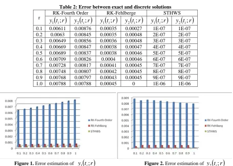
0.1 7.49966 10.76564 7.49355 10.75688 7.49931 10.76514 7.49966 10.76564 0.2 7.74158 10.64446 7.73528 10.63601 7.74123 10.64419 7.74158 10.64446 0.3 7.98350 10.52371 7.97701 10.51515 7.98314 10.52323 7.98350 10.52371 0.4 8.22543 10.40275 8.21874 10.39428 8.22505 10.40227 8.22543 10.40275 0.5 8.46735 10.28179 8.46046 10.27342 8.46697 10.28132 8.46735 10.28179 0.6 8.70928 10.16082 8.70219 10.15256 8.70888 10.16036 8.70928 10.16082 0.7 8.95120 10.03986 8.94392 10.03169 8.95079 10.03940 8.95120 10.03986 0.8 9.19313 9.91890 9.18565 9.91083 9.19271 9.91845 9.19313 9.91890 0.9 9.43505 9.79794 9.42737 9.78997 9.43462 9.79749 9.43505 9.79794 1.0 9.67698 9.67698 9.66910 9.66910 9.67653 9.67653 9.67698 9.67698

Table 2: Error between exact and discrete solutions

r RK-Fourth Order

( )

RK-Fehlberge STHWS

r

t

y

_{1 i}

;

y

₂

( )

t

_i

;

r

y

₁

( )

t

_i

;

r

y

₂

( )

t

_i

;

r

y

₁

( )

t

_i

;

r

y

₂

( )

t

_i

;

r

0.1 0.00611 0.00876 0.00035 0.00027 1E-07 1E-07 0.2 0.0063 0.00845 0.00035 0.00048 2E-07 2E-07 0.3 0.00649 0.00856 0.00036 0.00048 3E-07 3E-07 0.4 0.00669 0.00847 0.00038 0.00047 4E-07 4E-07 0.5 0.00689 0.00837 0.00038 0.00046 5E-07 5E-07 0.6 0.00709 0.00826 0.0004 0.00046 6E-07 6E-07 0.7 0.00728 0.00817 0.00041 0.00045 7E-07 7E-07 0.8 0.00748 0.00807 0.00042 0.00045 8E-07 8E-07 0.9 0.00768 0.00797 0.00043 0.00045 9E-07 9E-07 1.0 0.00788 0.00788 0.00045 0 1E-06 1E-06

Figure 1. Error estimation of

y

₁

( )

t

_i

;

r

Figure 2. Error estimation of

y

₂

( )

t

_i

;

r

From the graphical representation is given for the fuzzy hybrid differential equations shows that STHWS method approximate solutions have less error compare to Fourth Order Runge-Kutta method and Runge-Kutta Fehlberg method solutions [ ] in the all the stages.

6. CONCLUSIONS

In this paper, the single-term Haar wavelet series (STHWS) technique has been successfully employed to obtain the approximate analytical solutions of the fuzzy hybrid differential equation. Compare to Fourth Order Runge-Kutta method and Runge-Kutta Fehlberg method, STHW technique gives accurate results from the Table 1, Table 2. Also it is clear that from Table 2, Figure 1 and Figure 2 the STHWS method introduced in Section 4 performs better than Runge-Kutta method of Order Four and Runge-Kutta Fehlberg method.

REFERENCES

[1] Abbasbandy, S., Allah Viranloo, T., Numerical solution of fuzzy differential equation by Talor method, Journal of Computational Methods in Applied mathematics, 2 (2002), 113-124.

[4] Goetschel, R., Woxman, Elementary fuzzy calculus, Fuzzy Sets and Systems, 18 (1986), 31-43.

[5] Hsiao, C. F., and Wang, W. J., Haar wavelet approach to nonlinear stiff systems, Mathematics and Computation in Simulation, 57 (1998) 347-353.

[6] Jayakumar, T., Kanakarajan, K., Indrakumar, S., Numerical Solution of Nth-Order Fuzzy Differential Equation by Runge-Kutta Nystrom Method, International Journal of Mathematical Engineering and Science, 1(5) (2012), 1-13.

[7] Jayakumar, T., Kanagarajan, K., Numerical Solution for Hybrid Fuzzy System by Runge-Kutta Method of Order Five, International Journal of Applied Mathematical Science, 6 (2012), 3591-3606.

[8] Kaleva, O., Fuzzy Differential Equations, Fuzzy Sets and Systems, 24 (1987), 301-317.

[9] Kanagarajan, K., Sambath, M., Numerical Solution for Fuzzy Differential Equations by Third Order Runge-Kutta Method, International Journal of Applied Mathematics and Computation, 2(4) (2010), 1-10.

[10] Lakshmikantham, V., Liu, X.Z., Impulsive Hybrid systems and stability theory, International Journal of Nonlinear Differential Equations, 5 (1999), 9-17.

[11] Lakshmikantham, V., Mohapatra, R.N., Theory of Fuzzy Differential Equations and Inclusions, Taylor and Francis, United Kingdom, 2003.

[12] Ma, M., Friedman, M., Kandel, A., Numerical solutions of fuzzy differential equations, Fuzzy Sets and Systems, 105 (1999), 133-138.

[13] Pederson, S., Sambandham, M., The Runge-Kutta method for Hybrid Fuzzy Differential Equations, Nonlinear Analysis Hybrid Systems, 2 (2008), 626-634.

[14] Sambandham, M., Perturbed Lyapunov-like functions and Hybrid Fuzzy Differential Equations, International Journal of Hybrid Systems, 2 (2002), 23-34.

[15] Sekar, S., Manonmani, A., A study on time-varying singular nonlinear systems via single-term Haar wavelet series, International Review of Pure and Applied Mathematics, 5(2009), 435-441.

[16] Sekar, S., Balaji, G., Analysis of the differential equations on the sphere using single-term Haar wavelet series, International Journal of Computer, Mathematical Sciences and Applications, 4(2010), 387-393. [17] Sekar, S., Duraisamy, M., A study on CNN based hole-filler template design using single-term Haar wavelet

series, International Journal of Logic Based Intelligent Systems, 4(2010), 17-26.

[18] Sekar, S., Jaganathan, K., Analysis of the singular and stiff delay systems using single-term Haar wavelet series, International Review of Pure and Applied Mathematics, 6(2010), 135-142.

[19] Sekar, S., Kumar, R., Numerical investigation of nonlinear volterra-hammerstein integral equations via single-term Haar wavelet series, International Journal of Current Research, 3(2011), 099-103.

[20] Sekar, S., Paramanathan, E., A study on periodic and oscillatory problems using single-term Haar wavelet series, International Journal of Current Research, 2(2011), 097-105.

[21] Sekar, S., Vijayarakavan, M., Analysis of the non-linear singular systems from fluid dynamics using single-term Haar wavelet series, International Journal of Computer, Mathematical Sciences and Applications, 4(2010), 15-29.

[22] Seikkala, S., On the fuzzy initial value problem, Fuzzy Sets and Systems, 24 (1987), 319-330.

[23] Wu, C.X., Ma, M., Embedding problem of fuzzy number space Part I, Fuzzy Sets and Systems, 44 (1991), 33-38.