A PRELIMARY APPROACH FOR THE AUTOMATED RECOGNITION OF MALIGNANT MELANOMA

A PRELIMARY APPROACH FOR THE AUTOMATED RECOGNITION

OF MALIGNANT MELANOMA

E

Z

W

B

1_{D´epartement des sciences de l’informatique, Laboratory LIP2, Facult´e des Sciences de Tunis (FST), Campus}

Universitaire, 1060 Tunis, Tunisia,2_{Groupe du Recherche en Images et Formes de Tunisie (GRIFT), Laboratory}

CRISTAL, Ecole Nationale des Sciences de l’Informatique (ENSI), Campus Universitaire, 2080 La Manouba, Tunisia

e-mail: [email protected], [email protected]

(Accepted March 15, 2004)

ABSTRACT

In this work, we are motivated by the desire to classify skin lesions as malignants or benigns from color photographic slides of the lesions. Thus, we use color images of skin lesions, image processing techniques and artificial neural network classifier to distinguish melanoma from benign pigmented lesions. As the first step of the data set analysis, a preprocessing sequence is implemented to remove noise and undesired structures from the color image. Second, an automated segmentation approach localizes suspicious lesion regions by region growing after a preliminary step based on fuzzy sets. Then, we rely on quantitative image analysis to measure a series of candidate attributes hoped to contain enough information to differentiate melanomas from benign lesions. At last, the selected features are supplied to an artificial neural network for classification of tumor lesion as malignant or benign. For a preliminary balanced training/testing set, our approach is able to obtain 79.1% of correct classification of malignant and benign lesions on real skin lesion images.

Keywords: fuzzy region growing, Karhunen-Lo`eve transform, melanoma recognition, neural networks.

INTRODUCTION

The malignant melanoma is the most dangerous human skin disease. It is the deadliest form of all skin cancers and arises from cancerous growth in pigmented skin lesion. The incidence has increased dramatically during the last years. In the US, the incidence of melanoma is rising more rapidely than any other cancer. Data base available on the

internet (e.g. Nidus Information Services (2001):

http://www.ucdmc.ucdavis.edu/) report that since the early seventies, the melanoma has increased 126% in USA. In Europe, the malignant melanoma incidence is increasing by 5% every year and it is responsible of

91% of deathly skin cancer (Sboneret al., 2001).

If early recognized, the melanoma can be excised and the patient can recover completely. So one should intensify the awareness of all citizens. Indeed, the curability of skin melanoma is nearly 100% if recognized early enough, and treated surgically

(Pehamberger et al., 1987). The early diagnosis of

malignant melanoma is therefore a crucial issue for dermatologists. As a step towards improving early interpretation, a number of diagnostic checklists have

been proposed, including UK “Seven Point checklist”

(Healsmith et al., 1994), the American “ABCD” list

(Stolz et al., 1994), and “ABCDE” list (Fitzpatricket

al., 1988). The lists specify visual features associated

with malignant lesions symptoms. Unfortunately, it

can be difficult to interpret visually these features and then to recognize malignant pigmented lesion. Even experienced dermatologists have difficulties for distinguishing melanoma from other pigmented lesions of the skin, such as typical and atypical lesions whose are benign. In fact, correct detection rates based on clinical visual investigation is commonly about 65% (Lee, 2001).

This problem has stimulated interest in adjunctive diagnostic modalities that might facilitate clinical recognition of melanoma, including the automated interpretation of dermatoscopic color images with computerized image analysis. Thus, there has been

increasing interest in computer-aided systems (CAD)

for the clinical diagnosis of melanoma as a support for the dermatologists in different analysis steps, such as the lesion boundary detection, the quantification of diagnostic features, the classification in different types of lesions, the visualization, etc. Over the last few years, many works have developed allowing diagnostically useful systems based on image processing and recognition algorithms for atypical melanoma lesion. Readers interested in the current state of the art in computer aided image analysis in melanoma research, can refer to our precedent paper (Zagrouba and Barhoumi, 2003a).

main steps: image formation and preprocessing, segmentation, features extraction and classification of the lesion. In fact, after the acquisition and preprocessing of color images of the skin, the next step of the whole image analysis process is the segmentation of the lesion from the surrounding skin. The lesion areas and boundaries being clearly identified, various attributes of the lesion characteristic of the malignity symptoms must be measured. Such characteristic features will then be the raw input to a recognition algorithm classifying the lesion as melanoma or not. For a classification system to be successful, all four sub-tasks must be performed with care. The four steps are addressed in the next sections.

IMAGE FORMATION AND

PREPROCESSING

DATA DESCRIPTION

Dermatologists commonly use slides for lesion image storage and visual comparison. In this work, these slides were digitalized with a 35mm film scanner Nikon LS-1000. The resulting images that we used are BMP-format and are coded on 24 bits storing

the three color components r (red), g (green) and b

(blue). These rgb images are 150×150×3 pixels in

size, stored in 67 KBytes, with a spatial resolution of

0.0264 cm×0.0264 cm per pixel. Each image has one

or more lesions located near the center and the lesions are surrounded by normal skin of variable hue. Lesions can vary in size, shape, color and saturation. Fig. (1) shows the images of 4 different lesions. Lesions

a and b are benign nevus, however, lesions c and

d are malignant melanomas (Fig. 1). Other features,

such as hairs and pigments, can be observed in the images which can confuse the further analysis of the images. Thus, a preprocessing step is needed in order to ameliorate the image quality. It consists in reducing noise, strongly present in dermatoscopic images, and to enhance edges in order to eventually facilitate the separation between the lesion and the surrounding skin.

In our system, we applied a median filtering for minimizing the influence of small structures (like thin hairs) and isolated islands of pixels (like small air bubbles) in the segmentation result. For images including thick hairs with a color hue similar to the one of the lesion and thus irremovable by the median filter

(e.g.Fig. 1d), a specific hair removal technique (called

DullRazor (Lee et al., 1997)) is applied. The last preprocessing step in our system is the application of the Karhunen-Lo`eve transform that enhances the edges

towards making easier the extraction of the lesion from the surrounding skin.

(a) (b)

(c) (d)

Fig. 1. Color images of lesions. (a-b): benign nevus,

(c-d): melanomas.

MEDIAN FILTERING

Small structures and artifacts should be removed from skin images towards reducing the over-segmentation while at the same time preserving edges. These artifacts can be considered as impulsive noise and can be reduced using a median filter

(Hintz-Madsenet al., 1996) (e.g.Fig. 2).

(a) (b)

Fig. 2.Median filtering. (a) original image. (b) result

THICK HAIRS REMOVAL

This process is necessary only for images covered by thick hairs where the median filtering is insufficient

for hair suppression (e.g. Fig. 3). For these images,

more than 50% of the pixels in the current 5×5

pixel neighborhood scanned by the median filter could be hair pixels. The median value would be then representative of the hairs. Thus, the median filtering can intensify the undesired pixels which may degrade the segmentation process.

Fig. 3. Insufficiency of median filtering with a fixed

5×5neighborhood for thick hair removal. (a) original image. (b) result after median filtering: some hair structures are intensified.

Of course, shaving the hairs before imaging sessions may be a solution. However, this solution not only adds extra costs and time to the image session, but also is uncomfortable and impractical especially for multiple lesions or total-body nevus imaging (Voight and ClaBen, 1995). Hence, in spite of its algorithmic complexity, the preprocessing technique

called DullRazor (Lee et al., 1997) appeared to us

as the best solution, from a practical point of view, for thick hair removal. It consists in identifying hair areas and replacing hair pixels with nearby non-hair

pixels. In fact, for every pixelpa generalized grayscale

morphological closing operation is applied on the three color bands separately in order to localize the dark

hairs. In practice, for every color bandbk(k∈ {r,g,b}),

this operation approximates thick hairs shapes by smoothing out low intensity values along fixed-size structure elements in horizontal, diagonals and vertical

directions (e0,e45,e135 ande90) representing classical

hair forms. The generalized grayscale closing image

Gk is obtained by taking the maximum response from

the individual closing operations for each color band

(Eq. 1). Then, a binary hair maskHk image is created

by thresholding Gk. This hair mask divides the hair

and non-hair regions into disjoined areas. Finally, the

global binary hair mask (H) is the union⊕of all three

hair masksH=H_r⊕H_g⊕H_b(e.g.Fig. 4a).

∀k∈r,g,b,∀p,Gk(p) =|bk(p)−max(cp)|,

cp=[bk•e0](p),[bk•e45](p),

[bk•e90](p),[bk•e135](p) , (1)

where•denotes the grayscale closing operation.

(a) (b)

(c)

Fig. 4.Tick hairs removal. (a) hair mask H of Fig. 3a.

(b) the cleaned mask H0 _{relatively to H. (c) cleaned} image of Fig. 3a.

Before the replacement is performed, each pixel in the hair mask is checked to ensure that it is located within a thick and long structure (i.e hair structure); otherwise, the pixel is rejected as noise. In fact, for

each pixel inside the hair regionH, line segments are

drawn in 8 directions, up, down, left, right and the four diagonals, radiating from the concerned pixel until the line segment reaches the non-hair region. These 8 line segments form 4 straight lines centred at the pixel. The length of each line is calculated and the longest one is noted. In our experiments, the longest line must be longer than 75 pixels and other lines must be shorter

than 35 pixels (e.g.Fig. 4b). Then, a cleaned maskH0

is obtained. In the last step, every pixelIm(i,j)verified

interpolationIn(i,j)of the two nearby non-hair pixels

Im(i1,j1)andIm(i2,j2)along the shortest line (Eq. 2).

In(i,j) =Im(i1,j1)∗_dd2((i,j),(i2,j2))

2((i,j),(i1,j1))+

+Im(i2,j2)∗_dd2((i,j),(i1,j1))

2((i,j),(i2,j2)) , (2)

withd2is the euclidean distance defined by (Eq. 3):

d2((i1,j1),(i2,j2)) =

q

|i₂−i₁|2+|j₂−j₁|2. (3)

KARHUNEN-LO `EVE TRANSFORM

The next preprocessing step consists in applying the Karhunen-Lo`eve transform aiming to facilitate the segmentation process by enhancing the edges in the image. The Karhunen-Lo`eve transform, also

called principal components analysis(Lo`eve, 1998),

is the projection of the three color components on the eignvectors of their covariance matrix. The covaraince

matrixCovof the three channels (RGB) is computed

as expressed by Eq. (4):

Cov=V·V

t_−mV·mt V

x·y =BΛB

t_{, (4)}

where (x,y) is the size of each color channel, V is

a 3×xy matrix of pixel-realizations of the 3 color

channels (Eq. 5), mV is the vector mean of the color

channels (Eq. 6), B= [b1 b2 b3] is a matrix whose

columns are the eigenvectors of the covariance matrix

andΛa diagonal matrix containing the eigenvalues of

Covin decreasing order:λ1≥λ2≥λ3.

V =





r(1,1) .. r(1,y) r(2,1) .. r(x,y) g(1,1) .. g(1,y) g(2,1) .. g(x,y) b(1,1) .. b(1,y) b(2,1) .. b(x,y)



,

(5)

mV =_xy1 . x

∑

y

∑





r(i,j) g(i,j) b(i,j)



. (6)

The Karhunen-Lo`eve transformation is given by (Eq. 7):

∀k∈ {1,2,· · ·,xy}, z_k=Bt (v_k−mV)

and T = (z1z2 · · · zxy) =





t1

t2

t3



 , (7)

wherevk is thekthcolumn vector inV andT contains

what is known as the principal components. The kth

(k=1,3) row of T, noted t_k, is referred to as thekth

principal component.

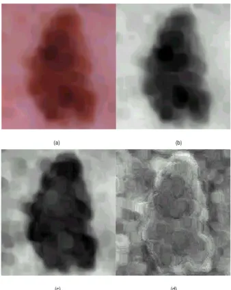
Due to the decreasing ordering of the eigenvalues and corresponding eignvectors, the first principal

component t1 will contain the maximum variance.

Since most variation occurs at edges between lesion and surrounding skin, the first principal component is a natural choice for segmentation. In fact, most of the texture and structure information will be mapped onto

the first principal component (e.g.Fig. 5). However,

although others principal components contain a small portion of the total variation, they may express features hidden in the original images.

(a) (b)

(c) (d)

Fig. 5.Results of the Karhunen-Lo`eve transform: (a)

the original median filtered color image, (b) the first principal component accounting for 92.29% of the total variance, (c) the second principal component – 7.63%, (d) the third principal lesion – 0.08%.

SEGMENTATION PROCESS

Several studies in the literature address the segmentation of dermatoscopic images, with most of them relying on color and grayscale thresholding

(Khanfir et al., 2002). However, the majority of

approach to localize suspicious lesion region in dermatoscopic images. It consists in determining the boundary of the lesion by region growing after an initial step based on fuzzy sets to enhance the lesion region of interest (ROI).

PREPROCESSING BASED ON FUZZY SETS

A typical first principal component of a median filtered dermatoscopic image consists of a very light background and a dark skin lesion with even darker areas inside. Herein, and as done elsewhere (Zagrouba

and Barhoumi, 2002; Rangayyan et al., 1997), we

have decided to characterize the lesion ROI working directly and only on the gray level intensities rather

than using other measurements (e.g.local gradients).

Then, a representative gray levelgl of the lesion must

be chosen.

In agreement with the intuitive idea that the relevant classes may correspond to the dominant peaks in the gray level histogram, our objective is to obtain a non ambiguous bimodal histogram expressing the

two following classes: lesion (class 1) and surrounding

skin (class 2). Along that line, starting from the noisy

bimodal histogram h of the t1 image (Fig. 6a), we

applied a succession of local smoothings of type Eq. (8), yielding to the smoothed bimodal curve (Fig. 6b).

This curve is characterized by two significant peaksh1

andh2and their corresponding gray levelsgl1andgl2

assumed to be representative of the gray levels of the two classes. Since the lesion is always darker than the

surrounding skin, its gray levelgl shall be the lower,

i.e.the minimum ofgl1andgl2.

h(i)← 1

3[h(i−1) +h(i) +h(i+1)]. (8)

(a) (b)

Fig. 6.histogram smoothing. (a) histogram of the first

principal component image, (b) the smoothed bimodal curve.

The enhancement of the ROI may be achieved by defining an appropriate membership function that evaluates the similarity between the properties of any

current pixel and those of the ROI itself (gl). Thus,

the original image t1 will be mapped to a fuzzy

set according to a symmetric membership function, decreasing monotonically from 1 to 0, and assigning

a membership of 1 to pixels of gray level gl. The

selected function has been defined after a study of many classical membership functions (Zagrouba and Barhoumi, 2003b) and is expressed by Eq. (9) where

β defines the opening of the membership function.

The contrast of the ROI in the resulting image depends

strongly upon theβ value. The largerβ, the more the

function is strict; the smallerβ, the more the function

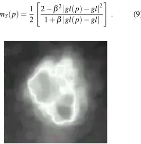
is permissive. Fig. (7) expresses the resulting fuzzy set

obtained with a small value for β (β =0.007). The

obtained fuzzy set represents pixels whose properties are close to the lesion with a high membership degree.

mS(p) =1₂

"

2−β2|gl(p)−gl|2

1+β|gl(p)−gl|

#

. (9)

Fig. 7.Enhancement of the ROI: white pixels are close

to 1. Note that the fuzzy image has been rescaled to enhance the visual quality.

LESION DETECTION BY REGION GROWING

We propose to obtain the lesion ROI and its associated boundary by performing region growing upon the obtained fuzzy set image. Region growing is a segmentation technique that gathers pixels into an homogeneous region according to a similarity criterion. This algorithm needs a seed pixel that

lies inside the ROI and a threshold θ as a stopping

are inspected and the procedure continues. If the connected pixel is less than the threshold, it is labeled as zero, indicating a boundary pixel, and its neighborhood are not processed. The recursive process continues until all connected pixels fail the test of inclusion in the region.

In order to optimize the region growing results, we wish to select the center of a homogeneous area as the

seed pixel. For this, given the setξ of pixels havinggl

as gray level, the seed pixelSis selected according to

the criterion defined by Eq. (10) (Fig. 8).

|gl−m(S)|=min

p∈ξ|gl−m(p)|. (10)

Where m(p) is the mean gray level of a 5×5 pixel

neighborhoodV(p)centered at pixel p.

(a) (b)

Fig. 8.Seed pixel determination. (a) the setξ of lesion

pixels having gl1 as gray level, (b) the seed pixel

location.

After the region growing process, a postprocessing

step ofDilatation-Erosion is done in order to remove

isolated pixels inside the lesion’s region (e.g.Fig. 9).

At the end, the out-put of the lesion extraction procedure is the so-called binary plane (Fig. 9c) that separates lesion from the healthy surrounding

skin. The resulting binary image (lesion vs. healthy

surrounding skin) will be then treated by an algorithm of follow-up (Barhoumi and Zagrouba, 2002) applied to the border pixels of the lesion characterized by a local maximum of gradient. It allows the definition of a polygon representing an approximation of the lesion

contourC.

(a) (b) (c)

Fig. 9.Region growing process. (a) original image, (b)

detection of the ROI lesion by region growing, (c) ROI after postprocessing of Dilatation-Erosion.

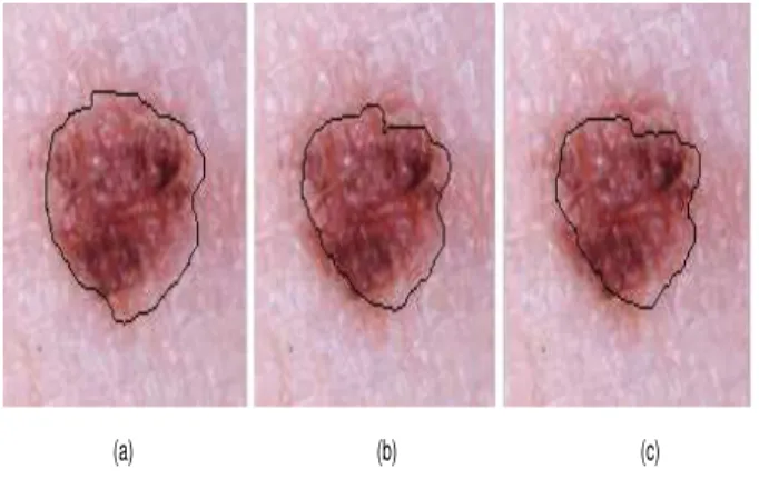
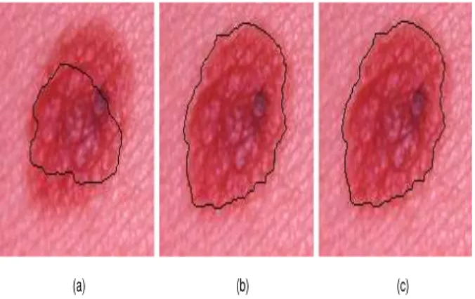
The parameters used in our segmentation

algorithm, β and θ, must be adequately chosen in

order to stop region growing at the boundaries of well-circumscribed lesions, where the membership values are expected to drop sharply across the lesion

boundary (e.g. Figs. 10-11). In our study, optimal

results are obtained with the values β =0.007 and

θ=0.75. In conclusion, our algorithm of segmentation

is simple and easy to implement and will always produce connected region and closed boundary. The binary object and its closed boundary are the basis to compute the vector of numerical features, which is the purpose of the feature extraction module.

(a) (b) (c)

Fig. 10. Original rgb image superimposed with the

boundary for various β values (θ =0.75). (a) β =

(a) (b) (c)

Fig. 11. Original rgb image superimposed with the

boundary for variousθ values (β =0.007). (a) θ=

0.5, (b)θ=0.7, (c)θ=0.95.

DERMATOSCOPIC FEATURE

DESCRIPTION

The essential difficulty in melanoma recognition systems is to design robust and relevant parameters describing the lesions in order to ensure the separation between melanoma and benign lesions, in particular atypical benign ones which may be clinically mistaken

for melanoma. We used the mnemonic device,ABCD,

to describe several features that help to distinguish melanomas from noncancerous growths. The choice

for the ABCDrule is based primarily on the fact that

the dermatologists we are working with use such rule. It shall be noticed that some studies report that the

ABCD rule may not yield the highest performance

in melanoma diagnostic compared to alternative

strategies such as stratification methods (Lorentzenet

al., 2000). Yet, the diagnostic performance depends

more on the selected attributes to represents the rule criteria, charaterizing the malignity symptoms, than

on the used rule itself (Ganster et al., 2001) so that

identifying the relevant ABCD features is definitely worth the effort. The different letters stand for the following criteria:

– Asymmetry (A): about half the time, a melanoma develops in an existing mole; in other cases, it arises as a new lesion that can resemble an ordinary mole. A noncancerous mole, however, is generally symmetric and circular in shape, while melanoma usually grows in an irregular, asymmetric manner.

– Border Irregularity (B): benign lesions generally have clearly defined borders. A melanoma, in contrast, often shows notched or indistinct borders that may signal ongoing growth and spreading of the cancer.

– Color Variation (C): one of the earliest signs of melanoma may be the appearance of various colors within the lesion. Because melanomas arise within pigment-forming cells, they are often varicolored lesions of tan, dark brown, or black, reflecting the production of melanin pigment at different depths within the skin.

– Diameter (D): early melanomas tend to grow larger than common moles and show typically at

least a diameter of about 6mm.

ABCDrules are commonly used by dermatologists.

Yet a diagnosis made by a dermatologist based on the visual and qualitative evaluation of such criteria may

be subjective (Schmid-Saugeon et al., 2003). Thus,

our main purpose is to charaterize the ABCDcriteria

by quantitative attributes measured by image analysis and then used as input to an automate classifier. In the literature, many attributes have been used to describe these features. A previous study by the authors (Zagrouba and Barhoumi, 2003a) of various attributes revealed some correlation between every single attribute and the melanoma diagnosis. However, each attribute alone is not sufficient to diagnose a lesion precisely. In other words, a combination of a set

of p(p>1 in general) relevant attributes is necessary

for the quantification of every feature and then for the diagnostic decision.

In Zagrouba and Barhoumi (2003b), we used 14

parameters describing the ABCD rule and yielding

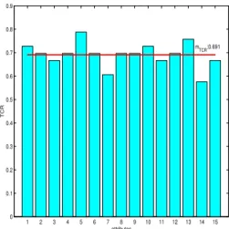
83% correct classification using a neural network classifier. This rate is related to a test subset of a series of images randomly selected from a database of 200 lesion images. However, this high number of attributes increases the classification complexity and the CPU time. We decided accordingly to define a reduced number of well-selected attributes permitting to obtain a higher correct classification rate while reducing the complexity and the CPU time by removing the redundant information. We will present, relatively to every feature, the adequate attributes that were chosen after many experiments and discussions with dermatologists. In fact, we realized a statistical study of 15 parameters (the 14 used in Zagrouba and Barhoumi (2003b) along with the

diameter) representing the four criteria (Barhoumi et

al., 2003). We classified a set of 100 lesion images

by using a neural network classifier considering every attribute separately. For simplicity reasons, we chose a simple training set of images composed of 50 significant melanomas, 50 significant benign lesions and 0 atypical lesions images. Then, we measure for

every attribute the correct classification rate (TCR)

relatively just to the chosen training set (this could

some attributes, e.g. Fig. 12). We kept only the attributes having a correct classification rate greater

or equal to mTCR with mTCR is the mean value of

the 15 TCR. In other words, we do not keep the

attributes whose shall decrease the global diagnostic performance. Besides, we decided not to use the lesion diameter (attribute number 5) since it is indirectly integrated in the other attributes. Thus, the set of 9 attributes discussed below was selected.

1 2 3 4 5 6 7 8 9 10 11 12 13 14 15

0 0.1 0.2 0.3 0.4 0.5 0.6 0.7 0.8 0.9

m_TCR:0.691

attributes

TCR

Fig. 12.Statical study of the correct classification rates

of15attributes using a NN classifier.

ASYMMETRY QUANTIFICATION

In order to measure asymmetry, we rely hereafter on geometrical properties called inertial moments

(Sonkaet al., 1993). Such inertial moments are used

to calculate two features: the asymmetry indexAI and

the lengthening index ˚A.

Asymmetry index

As far as asymmetry quantification is concerned, the origin of the local Cartesian basis is the center of

mass G of a current lesion L described by a binary

function z(i,j) (z(i,j) =1 if (i,j)∈L, 0 otherwise).

The quadratic inertial centred moment I(ϕ) of the

lesion L with respect to an arbitrary axis through G

showing an angleϕ with the horizontal Cartesian axis

∆is given by Eq. (11):

I(ϕ) =

∑

(i,j)∈L

D2 ϕ(i,j)

=

∑

(i,j)∈L

−isinϕ+jcosϕ

2

, (11)

where Dϕ(i,j) is the distance between a current

pixel (i,j) and its projection on ∆, along a direction

normal to ∆. The major principal axis is associated

to the smallest inertia moment ofL and provides the

longitudinal direction,ϕ0, ofL. It may then be obtained

by computing the derivative of Eq. (11) and setting it to zero as expressed by Eq. (12):

∂I(ϕ)

∂ϕ =0=⇒ϕ0=12tan−1

2mc

11

mc

20−mc02

, (12)

wheremc

11,mc20andmc02represent the standard product

moment, the quadratic moment with respect to the

horizontal Cartesian axisGxand the quadratic moment

with respect to the vertical Cartesian axisGy.

The minor principal axis of L associated to the

direction ϕ0+π/2 yields the transverse direction of

L associated to the largest moment of inertia. The

obtained longitudinal and transverse axes ofLmay be

used to calculate the asymmetry index. This is done

by folding the lesion L about these orthogonal axes

and measuring the area of non overlap as expressed by

Eq. (13) (e.g.Fig. 13):

AI=1

2

2

∑

∆Ak

AL , (13)

where the subscript k identifies the principal axis

(major vs. minor), ∆Ak is the corresponding

non-overlapping area of the folded lesion and AL (AL =

mc

00) is the lesion area.

Fig. 13.Skin lesion image showing the two principal

axes used to calculate asymmetry index. These axes define directions of smallest and largest moments of inertia. The asymmetry index for this lesion is 0.1796.

Lengthening index

This measure is used to describe the lengthening

of a lesion, i.e. the degree of anisotropy of a lesion.

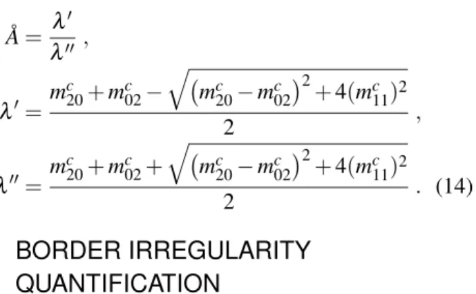
Lengthening of a lesion is related to the eigenvaluesλ0_,

ratio of the inertial momentλ0_{about the major axis by}

the inertial momentλ00_{about the minor axis (Eq. 14):}

˚

A= λ 0

λ00 ,

λ0₌m

c

20+mc02−

q

mc

20−mc02

2

+4(mc₁₁)2

2 ,

λ00₌m

c

20+mc02+

q

mc

20−mc02

2

+4(mc

11)2

2 . (14)

BORDER IRREGULARITY QUANTIFICATION

The irregularity of a lesion border has been presented as a very significant diagnostic factor when

assessing a lesion for malignancy (Keefeet al., 1990).

In this work, we used five features to quantify the border irregularity. These features are: compactness

index CI, fractal dimension f d, edge abruptnessCr

and pigmentation transitionme andve.

Compactness index

The compactness index(CI) (Eq. 15) is the most

popular border shape measurement estimating the roundness of a 2D object. However, this measure is very sensitive to noise along the border which is amplified by the square term of the perimeter (Lee, 2001):

CI= P

2

L

4πAL , (15)

wherePLis the perimeter of the lesion.

Fractal dimension

Extending from single-scale methods, the fractal

dimension (f d) is an elegant multi-scale method

showing a high correlation with the human intuitive

notion of roughness for curve lines (Tamura et al.,

1978; Pentland, 1984). The fractal concept is based on the fact that different results are obtained when classical geometrical curves and fractal curves (such as coast lines) are measured using rulers of various

size. For the first ones, the measured length`converges

to its true value as the ruler size r decreases (Eq.

16). However, for the second ones ` increases as r

decreases. The inverse relationship between ` and r

is due to the fact that many bays and promontories

smaller than the ruler sizerare unnoticed and omitted

(Mandelbrot, 1982); they become noticeable if the unit

sizerdecreases:

`=λr1−f d, (16)

where λ is a scaling constant and f d is the

characteristic of the coastline known as fractal

dimension. The value of f dis a fractional number that

is larger than or equal to the Euclidean dimension of the object.

Many studies have used the fractal dimension to estimate the irregularity of lesion border (Ng and Lee, 1996). The application of this measure to pigmented skin lesions showed that probability of a lesion being malignant increased with increasing fractal dimension,

and hence border irregularity (Claridge et al., 1992;

1998). The box counting method is one of the most popular techniques to estimate the fractal dimension

of a given curve`. The number of boxesN(r)of sizer

required to cover`has the following relationship (Eq.

17):

N(r)∝ 1

rf d . (17)

Thus, we used a square grid dividing the image into

pixels of sizer x r (e.g.Fig. 14).N(r)was evaluated

as the number of pixels containing a piece of the lesion

boundary. Different pixel sizesrwere used andf dwas

obtained as the slope of the regression line of log(r)vs.

log(N(r)).

Fig. 14. Calculation of the fractal dimension ( f d)

using the box counting method.

Edge abruptness

A lesion with irregular border has a large variance

in the radial distance (i.e.the distance d2 between its

centroidGLand boundaryC). Guthowicz-Krusinet al.

(1997) estimated border irregularity by analyzing the variance of the radial distance distribution (Eq. 18):

Cr=

1

PL∑p∈C(d2(p,GL)−md)

2

m2

d

, (18)

where md is the mean of the distanced2 between the

Pigmentation transition

This important feature describes the transition of the pigmentation between the skin lesion and the surrounding skin. A sharp abrupt edge suggests malignancy while a gradual fading of the pigmentation

indicates a benign lesion (Hintz-Madsenet al., 1996).

For this, we consider the luminance component

lum(i,j)(Eq. 19) of the original color image as just an equally weighted sum of the three color components. Then, we estimate the gradient magnitude of the

intensity component lum along the boundary C of

the skin lesion. We obtain a set of K gradient

magnitude values e(k) (1 ≤k ≤K, where K is the

number of boundary samples) describing locally the transition between the lesion and the skin background at each edge point. To describe more globally the

transition, we used the meanmeand varianceveof the

gradient magnitude valuese(k)describing globally the

abruptness level and its variation (Eq. 20).

lum(i,j) =1

3[r(i,j) +g(i,j) +b(i,j)]. (19)

me=_K1 K

∑

e(k), ve=_K1 K

∑

e2(k)−m2_e. (20)

COLOR VARIATION QUANTIFICATION

To further constrain the diagnosis, color variations in a lesion are here described by the color homogeneity

Ch and the correlation between geometry and

photometryCpg.

Color homogeneity

The luminance histogram of the lesion is divided into three intervals of equal length. The interval relating to the third smallest (resp. highest) luminance values defines the dark (resp. clear) areas in the lesion (Fig. 15); the intermediate interval relates to the rest of the lesion and does not participate in color quantification (Fig. 15). Then,

color homogeneityCh (Taouilet al., 2002) is defined

as the number of transitions clearer zone/darker zone and darker zone/clearer zone when scanning the lesion horizontally and vertically.

(a) (b)

Fig. 15.Evaluation of the color homogeneity. (a) initial

image, (b) the3color zones of the lesion used for the color homogeneity measure.

Correlation between geometry and photometry

This attribute evaluates the color distribution on the lesion. It consists in describing the evolution of the

color level from the centroidGLtowards the boundary

of a lesion (Eq. 21). This value is greater for benign lesions since they have a targeted aspect, while low values are signs of malignancy.

Cpg=_A1 L._p

∑

(lum(p)−m_l).(d₂(p,G_L)−m_d)

vl.vd ,

(21)

where md and vd are the mean and variance of the

distanced2introduced in Eq. (18),ml andml relating

to the luminance.

CLASSIFICATION PROCESS

The last step of our strategy consists in training a classification process with the feature attributes selected above. On the one hand, several techniques of classification, such as K-Nearest Neighbors (KNN)

(Ganster et al., 2001), Fuzzy C-Means (FCM)

(Cucchiara and Grana, 2002) and decision tree (Sboner

et al., 2001), have been applied to diagnose skin lesions. On the other hand, dermatologists base their clinical diagnostic decisions on experience as well as on complex inferences and extensive pathophysiological knowledge. Such experience can not be condensed into a small set of relations and this may limit the performance of algorithmic approaches

(Ercal et al., 1994). Experience-based learning is the

ours. Besides, as illustrated by many previous studies

(Binder et al., 1994; Ercal et al., 1994), neural

networks (NN) may result in reduced error rates for the melanoma diagnosis problem when compared to strictly algorithmic approaches. NN approaches are also a very flexible means for mapping a fixed number of inputs into a set of discrete classes. Such characteristics motivated the use below of a NN approach towards mapping a series of sample attribute values into two diagnostic classes (cancerous lesions, healthy lesions).

NEURAL NETWORK IMPLEMENTATION

In the last two decades, NN have been extensively used for classification applications. In fact, the classical approach to classification is statistical and concerns the modeling of stationary class-conditional probability distribution by a set of basis functions (Ripley, 1996). The most common neural network architecture for supervised classification is the

multi-layer perceptron (Rumelhartet al., 1988). It possesses

the importantuniversal approximationcapability, i.e.,

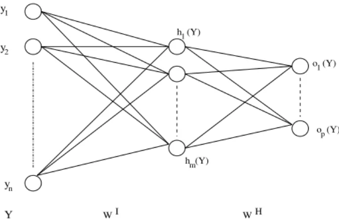
it may approximate any given function with arbitrary precision as long as the number of hidden-units is large enough. Thus, the multi-layer perceptron is the type of network that best fits our diagnosis application. After many tests with a different number of hidden layers, we decided to use a mono-layer perceptron yielding a satisfactory performance in a minimum training time. It may be represented by the network diagram in (Fig. 16).

y₁

y

y

2

n

1

h (Y)

h (Y)

o (Y)

m

1

o (Y)_p

I

W W H

Y

Fig. 16.Mono-layer perceptron structure.

The mono-layer perceptron is typically defined by sigmoidal hidden unit basis functions and by linear output functions. In this work, the chosen hidden activation function are hyperbolic tangent functions.

Thus, the output of the hidden units for a pattern Y

(Y = (y1,y2,· · ·,yn); n: number of input attributes)

may be expressed as Eq. (22):

∀j∈ {1,2,· · ·,m}, h_j(Y) =tanh

n

∑

wI

jiyi+wIj0

!

,

(22)

wherewI

jiis the weight connecting inputiand hidden

unit j,wI

j0 is the threshold for hidden unit j andmis

the number of units in the hidden layer.

The hidden unit outputs are weighted and summed yielding the following unbounded network outputs Eq. (23):

∀k∈ {1,2,· · ·,p}, o_k(Y) =

m

∑

wH_{k j}hj(Y) +wHk0,

(23)

wherewH

k j is the weight connecting hidden unit j and

the unbounded output unit k,wH

k0 is the threshold for

the unbounded output unitkand pis the units number

in the output layer.

In our case, the network architecture is defined by 9 input units representing the 9 selected attributes

describing the malignity symptoms (AI, ˚A, CI, f d,

Cr, me, ve, Ch and Cpg), m hidden units and one

linear output unit (thresholding function) producing a binary result (1 for a malignant lesion and 0 for a nonmalignant lesion). The attributes show different units and range values. Towards normalizing all attributes between 0 and 1, an objective scaling was

performed by calculating the corresponding z-scores

(Kaufman and Rousseeuw, 1996).

In our case, to approximate the classification function of a lesion as either benign or malignant, the back-propagation algorithm minimizes the squared

error εr between current outputs of the network and

the desired ones given with the training data. The training process allows the perceptron to learn and gain experience about the melanoma diagnosis problem in order to automatically classify correctly skin lesions other than those included in the training set. The

training continues till either the errorεr is lower than

0.1 or 10,000 iterations are executed which ensures the

convergence of the perceptron to a global solution. Furthermore, there are a number of arbitrary parameters whose values need to be defined carefully if the perceptron is to provide good performance. In particular, the number of hidden units largely affects the ability of the perceptron to determine the properties of patterns which are not members of the training

set (Bostock et al., 1993). In fact, the gap between

the approximation achieved by a neural network and the classification function to approach is inversely proportional to the number of hidden neurons (Barron, 1993). Unfortunately this result is not constructive, in the sense that it can only give vague estimations of the number of necessary hidden neurons. Thus, it does not exist at present time theoretical arguments to predict the number of necessary hidden units, to get a specified performance of the model, held account of the available data (Dreyfus, 2002). Thus, we varied the number of hidden units until optimal performance on the test set was obtained.

EXPERIMENTS AND RESULTS

The data set used herein consists of 200 images representing 75 representatives malignant lesions and 125 representatives benign ones. To evaluate the classifier performance of the designed perceptron, we

used the holdout method (Huberty, 1994) which is

the simplest kind of cross validation models. This method indicates how well the classifier will do when it is asked to make new predictions for data it has not already seen. It consists in separating the images data set into two disjoint and independent

sets, called the training set T1 and the testing set

T2. The classification function approximator fits a

function using the training set only. Then, the function approximator is asked to predict the output values for the data in the testing set (it has never seen these output values before). The errors it makes are accumulated as before to give the mean absolute test set error, which is used to evaluate the classifier performance. The evaluation may depend heavily on which data images end up in the training set and which end up in the test set, and thus the performance evaluation of the

perceptron may be significantly different depending on how the division is made. On the one hand, the size of the training set should be large enough to ensure a good classification rate. On the other hand, the size of the testing set should be also large enough to increase the confidence in the results (estimation of general performance). Herein we chose to use training and testing sets of comparable sizes; the following training

T1 / testing T2 percentiles (κ) were used: 40/60,

50/50 and 60/40 (Table 1).

The obtained results are summarized in Table 1 for

different number of hidden units (n) so that the effect

of architecture on performance could be assessed. This table records correct detection rates, using the

perceptron classifier, on the training set T1 (TCR1)

and on the testing set T2 (TCR2). Besides, accuracy

of classification on the testing set is evaluated in terms

of sensitivity sn2 (percentage of malignant lesions

correctly classified) and specificitysp2 (percentage of

benign lesions correctly classified). For each couple

(κ,n), the network weights are initialised randomly

over [−1,1] in every run and the final result, given

in Table 1, is computed as the average over a set of 10 runs. In Fig. 17, the results of a typical run of the designed algorithm of classification is shown.

0 10 20 30 40 50 60 70 80

0.5 0.6 0.7 0.8 0.9 1 1.1 1.2

iteration εr

training testing

Fig. 17. Part of the results of a typical run of the

Table 1.Neural network diagnostic results (percentage success rates) as a function of the number of hidden units (n) and the trainingT1/ testingT2combination percentiles (κ).

κ n TCR1 sn2 sp2 TCR2

40/60 3 69.9 56.0 73.2 64.6

40/60 4 85.7 68.3 77.1 72.7

40/60 5 81.3 66.5 80.3 73.4

40/60 6 81.0 76.6 79.2 77.9

50/50 3 74.7 63.6 70.9 67.25

50/50 4 88.6 69.5 75.1 72.3

50/50 5 74.2 67.0 76.4 71.7

50/50 6 81.7 61.3 76.8 69.05

60/40 3 71.8 61.2 77.4 69.3

60/40 4 94.5 75.1 83.1 79.1

60/40 5 86.1 67.4 76.5 71.95

60/40 6 93.7 74.5 81.2 77.85

When we compare the success classification rates

(TCR1andTCR2) for the three studied training/testing

combinations (κ), we can conclude that the best results

are recorded for the 60/40 combination. Independently

of the hidden units number, this combination produces the higher mean of correct classification for both

training and testing sets (86.53%, 74.55%) when

compared with the 50/50 (79.8%, 70.08%) and

40/60 (79.48%, 72.15%) combinations. This may be

explained by the fact that the size of current database is so small, so that it appears more appropriate to exploit the maximum of data for the training step in order to generalize the network decision. Thus, a total of 120 (resp. 80) lesions were used in the training (resp. testing) set, including 45 (resp. 30) melanomas.

Given this training/testing combination, the perceptron architecture having 4 hidden units gave optimal performance, both on the training and testing

sets (72.14%, 67.05%) comparatively to these given

with 3 (89.6%, 74.7%), 5 (80.51%, 72.35%) and 6

(85.47%, 74.94%) hidden units architectures.

In conclusion, given the disposed database, the perceptron with one hidden layer composed of four units, trained on 120 lesion images and tested on 80 lesion images yielded the best results with correct

classification rate (TCR2) of 79.1%, sensitivity (sn2)

of 75.1% and specificity (sp2) of 83.1%. These

results are comparable with the detection rates of very experienced dermatologists. However, the relatively higher rate of specificity when compared with the sensitivity rate is believed to be the consequence of the higher number of benign lesions than of melanoma images characterizing our data base.

CONCLUSION AND FUTURE

WORK

In this study, we attempted to diagnose melanoma from color skin images using image processing techniques and an artificial neural network classifier. Towards that end, we relied on a preprocessing step essentially based on a median filter for its ability to remove noise and undesired components. Then, we performed a PCA like analysis to enhance edges. To extract the lesion from the image, an automated segmentation approach permitted to localize suspicious lesion region by region growing after a preprocessing step based on fuzzy sets. Then, after a study of several existing features describing the lesion malignity, a set of 9 attributes to distinguish melanoma from benign lesions was defined and methods to measure these attributes were described. Finally, a mono-layer perceptron was trained with these attributes in order to classify the lesion as melanoma or nonmelanoma.

Future studies will be carried out on the enlarged data set (483 dermatoscopic color images) so that a more rigorous evaluation of our approach can be made. Besides, we will try to extract a

more reduced attributes set, using subset feature

selectiontechniques, in order to keep the classification complexity low and to reduce the CPU time while at the same time preserving a high correct classification rate.

ACKNOWLEDGMENTS

We sincerely thank Mr. Patrick Vannoorenberghe, Laboratory PSI (Perception Systemes Information) – FRE CNRS2645, Univeristy of Rouen, France; who allowed us to recover the data set of color dermatoscopic images used in this article.

REFERENCES

Astion M.L, Wilding P (1991). Application of neural networks to the interpretation of laboratory data in cancer diagnosis. Clin Chem 38(2):34–8.

Barhoumi W, Zagrouba E (2002). Boundaries Detection Based on Polygonal Approximation by Genetic Algorithms. Knowledge-Based Intelligent Information Engineering Systems and Allied Technologies (KES 2002), Frontiers in artificial intelligence and applications, IOS Press 82(2):621–7.

Proceedings of Conf´erence Internationale Sciences Electroniques, Techniques de l’Information et des T´el´ecommunications, SETIT, Tunisia.

Barron A (1993). Universal approximation bounds for superposition of a sigmoidal function. IEEE Trans Inform Theory 39:930–45.

Binder M, Steiner A, Schwarz M, Knollmayer S, Wolff K, Pehamberger H (1994). Application of an artificial neural network in epiluminescence microscopy pattern analysis of pigmented skin lesions: A pilot study. Brit J Dermatol 130(4):460–5.

Bostock RT, Claridge E, Harget AJ, Hall PN (1993). Towards a neural network based system for skin cancer diagnosis, Third International Conference on Artificial Neural Networks, 372:215–9.

Claridge E, Hall PN, Keefe M, Allen J (1992). Shape analysis for classification of malignant melanoma. J Biomed Eng 14:229–34.

Claridge E, Morris JD, Hall PN (1998). Evaluation of border irregularity in pigmented skin lesions against a consensus of expert clinicians. Proceedings of Medical Image Understanding and Analysis, UK, 85–8. Cucchiara R, Grana C(2002). Using the topological tree

for skin lesion structure description. Knowledge-Based Intelligent Information Engineering Systems and Allied Technologies (KES 2002), Frontiers in artificial intelligence and applications, IOS Press, 82(1):166–70. Dreyfus G (2002). Les r´eseaux de neurones : pourqoui et pour quoi faire. R´eseaux de neurones - M´ethodologies et Applications, Eds Eyrolles, 1–64.

Ercal F, Chawla A, Lee HC (1994). Neural network diagnosis of malignant melanoma from color images. IEEE Trans Biomed Eng 41(9):837–45.

Fitzpatrick TB, Rhodes AJ, Sober A, Mihm M (1988). Primary malignant melanoma of the skin: the call for action to identify persons at risk, to discover precursor lesions, to detect early melanomas. Pigm Cell Res 9(1):110–7.

Ganster H, Pinz A, Rohrer E, Wildling E, Binder M, Kittler H (2001). Automated melanoma recognition. IEEE Trans Med Imaging 20(3):233–9.

Guthowicz-Krusin D, Elbaum M, Szwaykowski P, Kopf AW (1997). Can early malignant melanoma be differentiated from atypical melanocytic nevus by in vivo techniques? Part II. Automatic machine vision classification. Skin Res Technol 3:15–22.

Haykin S (1999). Neural networks: A comprehensive fundation. Upper Saddle Rever, New Jersey: Prentice Hall.

Healsmith MF, Bourke JE, Graham-Brown RC (1994). An evaluation of the revised seven-point checklist for the early diagnosis of cutaneous malignant melanoma. Brit J Dermat 130:48–50.

Hintz-Madsen M, Hansen LK, Larsen J, Drzewiecki KT (1996). Detection of malignant melanoma using neural classifiers. in solving engineering problems with neural networks, International Conference on Engineering Applications using Neural Networks EANN, Turku, Finland, 395–8.

Huberty CJ (1994). Applied discriminant analysis. New York: John Wiley and Sons, Inc.

Kaufman L, Rousseeuw P.J (1990). Finding groups in data. New York: John Wiley and Sons, Inc.

Khanfir I, Kallel A, Taouil K, Bouhlel MS, Kammoun L (2002). Segmentation d’images par seuillage d’histogrammes : Application `a l’analyses de m´elanomes. JTEA’2002, Tunisia, 190–8.

Keefe M, Dick D, Wakkel R (1990). A study of the value of the seven-point checklist in distinguishing benign pigmented lesions from melanoma. Clin Exp Dermatol 15:167–71.

Lee KT, Gallagher R, Coldman A, McLean D (1997). Dullrazor: A software approach to hair removal from images. Comput Biol Med 27:533–43.

Lee KT (2001). Measuring border irregularity and shape of cutaneous melanocytic lesions. PhD, Simon Fraser University, Canada.

Lo`eve M (1998) Fonctions al´eatoires de second ordre. Levy P, editor, Processus Stochastiques et Mouvement Brownien, Hermann.

Lorentzen H, Wiesmann K, Kenet RO, Secher L, Larsen FG (2000). Comparaison of dermatoscopic ABCD rule and risk stratification in the diagnosis of malignant melanoma. Acta Derm-Venereol 80(2):122–6.

Mandelbrot BB (1982). The fractal geometry of nature. New York: W.H. Freeman and Co.

Ng V, Lee T (1996). Measuring border irregularities of skin lesions using fractal dimensions. In SPIE Photonics China, Electronic Imaging and Multimedia Systems, Beijing, 64–72.

Pehamberger H, Steiner A, Wolff K (1987). In vivo epiluminescence microscopy of pigmented skin lesions. Pattern analysis of pigmented skin lesions. J Am Acad Dermtol 17(4):571–83.

Rangayyan RM, El-Faramawy NM, Desautels J, Alim OA (1997). Measures of acutance and shape for classification of breast tumors. IEEE Trans Med Imaging, 16(6):199–210.

Ripley BB (1996). Pattern recognition and neural networks. Cambridge University Press.

Rumelhart DE, Hinton GE, Williams RJ (1988). Learning internal representations by error propagation. In parallel distributed processing - explorations in the microstructure of cognition, 1:318–62.

Sboner A, Blanzieri E, Eccher C, Bauer P, Cristofolini M, Zumiani G, Forti S (2001). A knowledge based system for early melanoma diagnosis support. Proceedings of the 6th _{IDAMAP workshop - Intelligent Data Analysis}

in Medicine and Pharmacology, London, UK.

Schmid-Saugeon P, Guillod J, Thiran JP (2003). Towards a computer-aided diagnosis system for pigmented skin lesions. Computerized Medical Imaging and Graphics., 27:65–78.

Sonka M, Hlavac V, Boyle R (1993). Image processing, analysis and machine vision. London: Chapman & Hall. Stolz W, Braun-Falco O, Bilek P, Landthaler M, Cognetta AB (1994). Color atlas of dermatoscopy. Berlin: Blackwell Science Ltd.

Tamura H, Mori S, Yamawaki T (1978). Textual features corresponding to visual perception. IEEE Trans Syst Man and Cyb 8:460–73.

Taouil K, Bouhlel MS, Elloumi, Kammoun L (2002). Quantification des caract`eristiques de m´elanomes en vue d’une classification. JTEA’2002, Sousse Nord, Tunisia, 179–85.

Voight H, ClaBen R (1995). Topodermatographic image analysis for melanoma screening and the quantative assessment of tumor dimension parameters of the skin. Cancer 75(4):981–8.

Zagrouba E, Barhoumi W (2002). Semiautomatic detection of tumoral zone. Image Anal Stereol 21(1):13–8. Zagrouba E, Barhoumi W (2003a). Objective and

cost-efficient approach for skin lesions classification. Proceedings of the IEEE/ACS International Conference on Computer Systems and Applications, Gammarth, Tunisia, 135–6.

Zagrouba E, Barhoumi W (2003b). Systme d’aide au diagnostic du m´elanome pour les dermatologues. 1ere