PLANAR SECTIONS THROUGH THREE-DIMENSIONAL LINE-SEGMENT PROCESSES

PLANAR SECTIONS THROUGH THREE-DIMENSIONAL LINE-SEGMENT

PROCESSES

S

D

M

D

S

1_{Institut f¨ur Keramik, Glas- und Baustofftechnik, Technische Universit¨at Bergakademie Freiberg, D-09596}

Freiberg, Germany;2Institut f¨ur Stochastik, Technische Universit¨at Bergakademie Freiberg, D-09596 Freiberg, Germany

e-mail: [email protected]

(Received September 25, 2013; revised January 14, 2014; accepted January 14, 2014)

ABSTRACT

This paper studies three–dimensional segment processes in the framework of stochastic geometry. The main objective is to find relations between the characteristics of segment processes such as orientation- and length-distribution, and characteristics of their sections with planes. Formulae are derived for the distribution of segment lengths on both sides of the section plane and corresponding orientations, where it is permitted that there are correlations between the angles and lengths of the line-segments.

Keywords: fibre process, fibre-reinforced materials, line-segment process, stereology, stochastic geometry.

INTRODUCTION

Segment processes are stochastic models for random systems of line-segments randomly scattered in space. They belong to the more general class of fibre processes, the mathematical theory of which was developed by Joseph Mecke and coworkers (Mecke and Nagel, 1980; Mecke and Stoyan, 1980b; Chiuet al., 2013).

These processes find important applications in the context of fibre-reinforced materials, where fibres, which can be often modelled as line-segments of negligible thickness, are embedded in a matrix of more or less homogeneous material.

In the now classical papers mentioned above planar sections played an important role. Such sections produce systems of fibre–plane intersection points, which can be statistically analysed with the aim to get information on the spatial fibre system. This setting belongs to the field of stereology, and a classical formula there is

LV =2NA, (1)

whereLV is the mean total fibre length per unit volume

and NA the number of intersection points per unit

area. (The formula holds true under the assumptions of statistical homogeneity or stationarity and isotropy, see also Chiuet al., 2013.)

Planar sections through segment processes appear in the context of fibre-reinforced materials, when axial tension is studied. Following Li et al. (1991) the intersections of fibres with a plane orthogonal to the tension axis are investigated. Additionally to the characteristics studied when stereology is of interest,

also the residual lengths of the line-segments on both sides of the section plane are of importance in the mechanical calculations. (They have never been considered in the stereological context, since these lengths cannot be measured in the section plane.)

The present paper first explains a natural segment process model, following the pattern of Mecke and Stoyan (1980a). Then it derives formulae for the section process characteristics. Some of them have counterparts in the classical theory, while those related to the residual lengths are new, generalising results in Li et al. (1991), who considered the case of segments of constant length. Furthermore, formulae for the maximum and minimum residual segment length are derived since these characteristics play a role in calculations of the contribution of fibres to the mechanical strength in a composite material.

MODEL DESCRIPTION

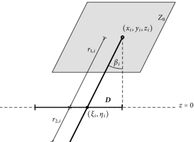
This paper considers three–dimensional line-segment processes. A realisation of such a process is a set of randomly distributed line-segments in space. To characterise such a line-segment we use its top point (in the sense of the z-axis) (x,y,z) ∈ R3, the

Figure 1.Computer-tomography-based measurements on fibre-reinforced autoclaved aerated concrete. The upper figure shows the three-dimensional distribution of fibres. The lower figure presents a planar section of reinforced material. The section points of the fibres (black points) form a random point pattern.

x y

z

λ β

l

Figure 2.Geometrical representation of a line-segment which is shifted so that its endpoint meets the origin of the coordinate system.

A line-segment process is here represented as a

marked point process ΨV (for more on marked point

processes see Chiu et al., 2013). Realisations of ΨV

can be written as sequences of marked points:

ψV ={[(xi,yi,zi),lVi ,λiV,βiV]}, (2)

with (xi,yi,zi) ∈ R3,lVi > 0,λiV ∈ [0,2π] and βiV ∈

0,π

2

. Moreover we introduce the stochastic variables of the polar angle, BV, the azimuthal angle, ΛV, and the fibre length,LV, of a typical line-segment ofΨV.

Here and in the following we assume ΨV to be

stationary, i.e., the distribution of ΨV is translation

invariant. It is not assumed that the marked point process ΨV has some specific distribution, e.g., a

marked Poisson process. The results presented in this paper hold for every distribution of a stationary ΨV,

where BV and ΛV are stochastically dependent (see page 57) or independent (see page 60) ofLV.

ESSENTIAL PROPERTIES

The distribution of the marked point processΨV is

described by the following characteristics:

Table 1. Characteristics of the spatial marked point processΨV

NV mean number of top points of

line-segments per unit volume

FV,L,B,Λ(l,β,λ) joint distribution function of fibre length LV and angles

BV and ΛV of a typical line segment

FV,B(β),FV,Λ(λ), FV,L(l)

marginal distribution functions of the stochastic variables BV, ΛV andLV.

The stochastic variables of the polar angle,BV, and the azimuthal angle,ΛV may depend on the stochastic variable of the spatial fibre length,LV.

In order to study the mechanical behavior of fibre-reinforced materials under axial tensions the intersection of a plane with a line-segment system is of peculiar interest. The mechanical effect of a fibre in a homogeneous material depends on the intersection angle and the length of the fibre under and over the plane respectively. Thus these quantities have to be studied. This approach appears in the classical papers by Liet al. (1991), Brandt (1985) and in subsequent work. However, in these papers the segment lengths are assumed to be constant.

Due to our homogeneity assumption we choose the intersecting plane to be the(x,y)-planeS={(x,y,z)∈

S yields the marked point process ΨA of intersection

points with the realizations

ψA={[(ξi,ηi),r_1,Ai,r A

2,i,λ A i ,β

A

i ]}, (3)

where (ξi,ηi) are the intersection points,rA_1,i and rA_2,i

the lengths of the upper and lower part of the segments respectively andλ_iA andβ_iA the corresponding section angles. Due to stationarity ofΨV also the marked point

processΨAis stationary.

We introduce the stochastic variables of the polar section angle, BA, the azimuthal section angle ΛA and the upper and lower part of the segment which belongs to the typical intersection point, RA₁ and

RA₂ respectively. The basic constants and distribution functions of the marked point processΨAare shown in

the following table:

Table 2. Characteristics of the planar marked point processΨA

NA mean number of section

points ofΨAper unit area

FA,R₁,R₂,Λ,B(r1,r2,λ,β) joint distribution function

of upper and lower segment lengths and intersection anglesBA,ΛA at a typical section point

FA,R₁,R₂(r1,r2), FA,Λ(λ),FA,B(β)

marginal distribution functions of the upper and lower segment lengths and the intersection anglesBAandΛA.

BASIC CHARACTERISTICS OF

Ψ

AND RELATIONS TO

Ψ

MAIN RESULTS

The main objective at this point is to establish relations between the basic constants and distribution functions ofΨV and those of ΨA. Due to the choice

of the intersection plane S and the definition of the azimuthal angleλ, the latter can be ignored.

We concentrate on relations between NA, NV and

the marginal distribution functionsFA,R₁,R₂,B(r1,r2,β)

andFV,L,B(l,β). The following general basic equation

holds forNA,NV >0,r1,r2>0 andβ ∈

0,π

2

:

NAFA,R₁,R₂,B(r1,r2,β) =

=NV

β Z

0

sinβ0

min{r₁,r₂}

Z

0

FV,L,B(l+max{r1,r2},β0)

−FV,L,B(l,β0)

dldβ0

+NVcosβ

min{r₁,r₂}

Z

0

FV,L,B(l+max{r1,r2},β)

−FV,L,B(l,β)

dl. (4)

The relation of the corresponding probability density functions fV,L,B(l,β) and fA,R₁,R₂,B(r1,r2,β) is

therefore

NAfA,R₁,R₂,B(r1,r2,β) =NVcosβfV,L,B(r1+r2,β).

(5)

Eq. 4 is the starting point for some important formulae. Letβ = π₂ andr1,r2→∞. Then we obtain

the intensity ofΨAas

NA=NVE(LVcosBV), (6)

where

E(LVcosBV) =

π 2

Z

0 ∞ Z

0

lcosβfV,L,B(l,β)dldβ.

This expression simplifies for the isotropic case and if

LV andBV are stochastic independent, see Eq. 26.

With the latter relation we are able to determine

FA,R₁,R₂,B ifNV andFV,L,B are given. Furthermore, we

obtain with Eq. 4, Eq. 6 andβ=π₂ the joint distribution function

FA,R₁,R₂(r1,r2) =FA,R₁,R₂,B

r₁,r₂,π

2

of the upper and lower segment lengths. These distributions exist if EcosBV 6=0, i.e., if the case of all fibres parallel to the section plane is excluded.

NAFA,R₁,R₂(r1,r2) =

=NV

min{r₁,r₂}

Z

0 π 2

Z

0

sinβ0 FV,L,B(l+max{r1,r2},β0)

−FV,L,B(l,β0)

dβ0dl, FA,R1,R2(r1,r2) =

= 1

E(LV_cosBV₎

min{r₁,r₂}

Z

0 π 2

Z

0

sinβ0·

FV,L,B(l+max{r1,r2},β0)−FV,L,B(l,β0)

dβ0dl,

with 0≤r1,r2 <∞. We can determine the marginal distribution functions for the upper and lower segment lengths

FA,R₁(r1) = lim

r2→∞

FA,R₁,R₂(r1,r2)

and

FA,R₂(r2) = lim

r₁→∞

FA,R₁,R₂(r1,r2).

The stochastic variables RA₁ and RA₂ are identically distributed with the distribution function

FA,R(r) =FA,R₁(r) =FA,R₂(r) =

1 E(LV_cosBV₎

r

Z

0 π 2

Z

0

sinβ0 FV,B(β0)

−FV,L,B(l,β0)dβ0dl, (8)

forr>0 andFV,B(β) =lim l→∞

FV,L,B(l,β).

With Eqs. 6 and 4 andr1,r2→∞we analogously get the distribution function of the section angleBA

FA,B(β) =

1 E(LV_cosBV₎

∞ Z

0

β Z

0

sinβ0 FV,B(β0)−FV,L,B(l,β0)

dβ0

+cosβ FV,B(β)−FV,L,B(l,β)

!

dl.

(9)

With Eqs. 6–9 we have explicit relations for the basic characteristics ofΨA. We can add also the probability

density functions using Eqs. 6–9:

fA,R₁,R₂(r1,r2) =

1 E(LV_cosBV₎

π 2

Z

0

cosβfV,L,B(r1+r2,β)dβ, (10)

and

fA,B(β) =

1 E(LV_cosBV₎

∞ Z

0 ∞ Z

0

cosβfV,L,B(r1+r2,β)dr1dr2.

(11)

The length of the line-segments were assumed to be stochastically dependent on the angle BV

throughout the above investigations. Eq. 4 shows that, consequently, the line-segment lengthsRA₁ andRA₂ are stochastically dependent of the intersection angleBA.

SKETCH OF THE PROOF OF EQ. 4

The proof follows the pattern of Mecke and Stoyan (1980a), which is also used in Mecke and Stoyan (1980c).

Let SD(t1,t2,b,c) be the expected number of

segments pi = [(xi,yi,zi),lV_i ,λ_iV,β_iV] of the marked point processΨV fulfilling the following conditions:

1. the line-segment pi intersects a given compact

subsetDof the planeS,

2. the line-segment has intersection anglesβ_iA∈[0,b] withb∈

0,π

2

andλ_iA∈[0,c]withc∈[0,2π],

3. the lengths of the segment above and belowSfulfil

rA_1,i≤t1andrA2,i≤t2witht1,t2>0.

The quantitySD(t1,t2,b,c) can be calculated in terms

ofΨA andΨV, and equating the corresponding terms

yields Eq. 4.

The Campbell theorem (see,e.g., Chiuet al., 2013) applied toΨA yields simply

SD(t1,t2,b,c) =NAFA,R₁,R₂,B,Λ(t1,t2,b,c) (12)

fort1,t2>0,b∈

0,π

2

andc∈[0,2π].

In terms ofΨV,SD(t1,t2,b,c)can be expressed as

SD(t1,t2,b,c) =E

∑

pi∈ψV

f(pi,t1,t2,b,c) !

(13)

for t1,t2 > 0, b ∈

0,π

2

and c ∈ [0,2π], pi =

[(xi,yi,zi),lV_i ,λ_iV,β_iV]denotes a single segment and f is the indicator function with f(pi,t1,t2,b,c) =1 for

segments that fulfil the conditions 1–3 of the definition ofSD, otherwise f =0. In the following we describe

the function f.

With r_1,A_i+rA_2,i =l_iV it follows 0≤lV_i ≤t1+t2 as

a first constraint. Furthermore we haveβ_iV ∈[0,b]and λ_iV ∈[0,c], therefore we choose

f(pi,t1,t2,b,c) =

1[0,t₁+t₂](lVi )1[0,b](βiV)1[0,c](λiV)1Z0(xi,yi,zi)

for some setZ₀=Z₀(λ_iV,β_iV,lV_i ,t1,t2)with(xi,yi,zi)∈

Z0if and only if pifulfils the conditions 1 and 3. Let

Z1=D⊕ n

s·e_λV

i ,βiV,s∈[0,min{l

V i ,t1}]

o

and

Z2=D⊕ n

s·e_λV

i ,βiV,s∈[l

V

i −min{l V

i ,t2},lVi ]

with e_λ,β = (cosλsinβ,sinλsinβ,cosβ), where ⊕ denotes the Minkowski addition. Thenpiintersects the

set D with an upper segment length rA_1,i ≤t₁ if and only if(xi,yi,zi)∈Z1and pi intersectsDwith a lower

segment lengthrA_2,i≤t₂if and only if(xi,yi.zi)∈Z2. In

both casespi intersectsDwith the intersection angles

β_iV ∈[0,b]andλ_iV ∈[0,c]. It follows thatpifulfils the

conditions 1 to 3 if and only if(xi,yi,zi)∈Z0=Z1∩Z2.

Due to the structure ofZ1andZ2we can writeZ0as the

Minkowski sum ofDand a line-segment:

Z₀=

D⊕ns·e_λV

i ,βiV,s∈[l

V

i −min{t2,lVi },min{t1,lVi }]

o .

Fig. 3 explains the underlying geometry.

βi

b

(xi,yi,zi)

z=0

D

Z0

(ξi,ηi)

r1,i

r2,i

Figure 3.Underlying geometry in the(x,z)-plane of the intersection of a segment of azimuthal angleλ_iV =0 with the plane S.

The right hand side of Eq. 13 can be calculated by means of the Campbell theorem. We obtain

SD(t1,t2,b,c) =

=NV

Z

R3

Z

[0,t₁+t₂]×[0,b]×[0,c]

1Z₀(x,y,z)·

dFV,L,B,Λ(l,β,λ)d(x,y,z)

=NV

Z

R3 t₁+t₂

Z

0

b

Z

0

c

Z

0

1Z0(x,y,z)

fV,L,B,Λ(l,β,λ)dλdβdld(x,y,z). (14)

By applying Fubini’s theorem we can rearrange the order of integration, and we evaluate

R

R3

1Z0(x,y,z)d(x,y,z) using Cavalieri’s principle. Due

to the representation ofZ0as a Minkowski sum we can

express this integral by the product of the area of D, ν2(D), and the height ofZ0. We get

Z

R3

1Z0(x,y,z)d(x,y,z) =

ν2(D)cosβ min{l,t1}+min{l,t2} −l

.

At this point the integrand is independent of λ. With Eq. 12 it follows the equivalence of the marginal distributions

FA,Λ(λ)≡FV,Λ(λ). (15)

Hence follows, we concentrate on the relation of the marginal distribution functions FA,R₁,R₂,B and FV,L,B

andSD(t1,t2,b,2π). We obtain

SD(t1,t2,b,2π) =

NV

Z

[0,t₁+t₂]×[0,b]

cosβ·

min{l,t1}+min{l,t2} −l

dFV,L,B(l,β).

(16)

Equating Eq. 16 with Eq. 12 and applying integration by parts gives the desired relation Eq. 4.

APPLICATIONS AND DISCUSSION

The stereological formulas Eqs. 6–9 can now be used to verify earlier results and to examine application-related cases.

SUPERPOSITION OF LINE-SEGMENT PROCESSES

In the following example the line-segments follow a special relation between length and direction: long fibres (l∈[l0,lmax], 0<l0 <lmax) all have the same

polar angle β0 ∈

0,π

2

while short fibres (l∈[0,l0])

are isotropic. The proportion of segments of length

l∈[0,l0]isp∈[0,1]and for segments withl∈[l0,lmax]

is 1−p. The joint probability density function ofLV

andBV is therefore

fV,L,B(l,β) =  



p

l0sinβ , l≤l0

1−p

lmax−l0δβ0(β), l0≤l≤lmax

0, l>l_max.

(17) Thus, this example represents a superposition of two different line-segment processes. With Eq. 6 the mean number of section points per unit area is

NA=NV

1 4pl0+

1

2cosβ0(1−p)(lmax+l0)

Moreover using Eq. 7 and Eq. 8 the conditional distribution function

FA,R₁|R₂≤r₂(r1) = min{r₁,r₂}

Z

0 π 2

Z

0

sinβ0 FV,L,B(l+max{r1,r2},β0)

−FV,L,B(l,β0)dβ0dl !,

r2

Z

0 π 2

Z

0

sinβ0 FV,B(β0)−FV,L,B(l,β0)

dβ0dl !

as well as the conditional density function

fA,R₁|R₂≤r₂(r1) = π

2

R

0

sinβ0 FV,L,B(r1+r2,β0)−FV,L,B(r1,β)dβ0

r₂

R

0 π 2

R

0

sinβ0 FV,B(β0)−FV,L,B(l,β0)dβ0dl

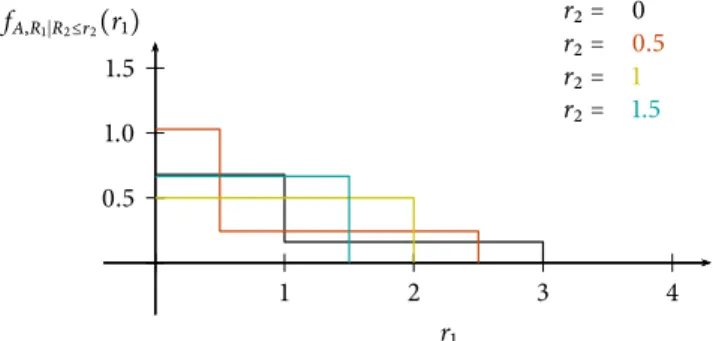
can be calculated. The conditional probability density function fA,R₁|R₂≤r₂(r1) is shown in Fig. 4 forl0=1, lmax=3,β0=3₄andp=3₄and by means of Eq. 18 the

ratio NA

N_V is 0.553. Thus,NAcan be determined onceNV

is known.

0.5 1.0 1.5

1 2 3 4

r2= 0

r2= 0.5

r2= 1

r2= 1.5

fA,R1∣R2≤r2(r1)

r1

Figure 4.The conditional probability density function fA,R₁|R₂≤r₂(r1) of the upper segment length RA1 under the condition the lower segment length RA₂ is bounded from above.

INDEPENDENT FIBRE ANGLES AND LENGTHS

Assume the line-segment length LV is stochastically independent of the anglesΛV andBV for the line-segment process ΨV. Under this assumption

this line-segment process can be characterized using the following parameters and functions:

Table 3. Characteristics of the spatial marked point processΨV under the assumption that LV and BV are

stochastically independent.

NV mean number of top points of

line segments per unit volume

FV,L(l) distribution function of length

of a typical segment ofΨV

FV,Λ(λ),FV,B(β) distribution function of azimuth

and polar angle of a typical segment ofΨV

Eq. 4 simplifies in the following way:

NAFA,R1,R2,B(r1,r2,β) =

=NV

min{r₁,r₂}

Z

0

β Z

0

FV,L(l+max{r1,r2})−FV,L(l)

·cosβ0dFV,B(β0)dl

=NV

min{r₁,r₂}

Z

0

FV,L(l+max{r1,r2})−FV,L(l)

dl

·

β Z

0

sinβ0FV,B(β0)dβ0

for r1,r2 >0, β ∈0,π₂ and NA,NV >0. It follows

that the segment lengths RA₁, RA₂ and the polar angle

BA of the segment process ΨA are stochastically

independent.

We therefore concentrate on the marginal distribution functionsFA,R₁,R₂(r1,r2)andFA,B(β). We

have

NAFA,R₁,R₂(r1,r2)FA,B(β) =

NV

min{r₁,r₂}

Z

0

FV,L(l+max{r1,r2})−FV,L(l)

dl·

β Z

0

sinβ0FV,B(β0)dβ0. (19)

Using this simplified relation we obtain

NA=NVELVEcosBV, (20)

FA,R₁,R₂(r1,r2) =

1 ELV

min{r₁,r₂}

Z

0

FV,L(l+max{r1,r2})−FV,L(l)

dl

and

FA,B(β) =

1 EcosBV

β Z

0

sinβ0FV,B(β0)dβ0. (22)

The segment lengths RA₁ and RA₂ are identically distributed, i.e., the marginal distributions FA,R₁ and

FA,R₂ are equivalent:

FA,R(r) =FA,R₁(r) =FA,R₂(r) =

1 ELV

r

Z

0

1−FV,L(l)

dl, r>0. (23)

Concerning the corresponding probability density functions ofΨV andΨAit holds

fA,R₁,R₂(r1,r2) =

1

ELV fV,L(r1+r2), (24)

and

fA,B(β) =

1

EcosBV fV,B(β)cosβ . (25)

THE ISOTROPIC CASE

We assume that the line-segment length LV is stochastically independent of the angles ΛV and BV

for the line-segment processΨV. Furthermore the

line-segment process ΨV is assumed to be isotropic, i.e.,

the directional vector of the typical line-segment is uniformly distributed on the unit sphere. We have

fV,B(β) =sinβ ,

and the distribution function

FV,B(β) =1−cosβ

for this case. Eq. 9 yields

fA,B(β) =sin 2β ,

and

FA,B(β) =sin2β ,

which is a result true for general fibre processes, see Mecke and Nagel (1980).

With Eq. 6 we obtain NA, the mean number of

section points per unit area as

NA=

1 2NVEL

V

. (26)

This result is a special case of another well-known stereological formula, namely (11.3.3) in Chiu et al.

(2013), where characteristics of germ-grain models are studied. Here the ”grain” is an isotropic line-segment.

SEGMENTS OF CONSTANT LENGTH

In papers such as Liet al.(1991) and Brandt (1985) line-segment processes and their sections with planes are studied. They derived formulas for the strength of fibre-reinforced materials using calculations for segments of constant length. If in this context the constant length is chosen to bel0>0, we obtain with

Eq. 8 the marginal distribution function FA,R(r). It

holdsFV,L(l) =Θ(l−l0)with the Heaviside function

Θ(x) =

0, x<0 1, x≥0

and

FA,R(r) =

1

l₀

r

Z

0

1−Θ(l−l0)

dl

=

r

l₀, r≤l0

1, r≥l₀

for the distribution function of the upper and lower segment length at a typical section point. This distribution is the uniform distribution on [0,l₀]. We therefore obtain the mean values of the residual segment lengths ERA₁ = ERA₂ = 1₂l0. This result

coincides with results of Liet al.(1991).

Moreover the line-segments in (Li et al., 1991) are considered to be isotropic. Using Eq. 26 we have

NA=1₂NVl0.

A PARAMETRIC MODEL

In Chin et al. (1988), Hegler (1985) and other papers line-segment length and angle distribution functions for segment processes ΨV with LV

independent ofBV appear such as

FV,L(l) =1−e−(ml)

k

, m,k,l>0,

the Weibull distribution function, and

FV,B(β) =

1−exp(−η β) 1−exp −π

2η

, β ∈ h

0,π

2

i

,η>0.

isotropic case. The Figs. 5 and 6 give an impression of the influence of the parameters m,k andη on the probability density functions fV,Land fV,B.

0.5 1.0

0.5 1.0 1.5 2.0

fV,L(l)

l

k=2 _m=0.5

k=2 _m=1

k=2 m=1.5

Figure 5.Influence of the parameters k and m on the Weibull probability densitiy function of LV.

1 2 3

1 8π

1 4π

3 8π

1 2π

β fV,B(β)

η=0 η=1 η=2 η=3

Figure 6. Influence of the shape parameter η on the probability density function of polar angle BV.

0.5 1.0

2 4 6 8 10

η

NA

NV

Figure 7. The ratio NA

N_V in dependence on shape

parameterη.

0.5 1.0 1.5

0.5 1.0 1.5 2.0

fA,R1∣R2≤r2(r1)

r1

r2=0.2

r2=1.2

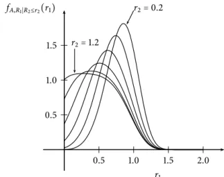
Figure 8.The conditional probability density function fA,R₁|R₂≤r₂(r1) in dependence on r2 for Weibull-distributed fibre lengths. This is the probability density function of the length RA₁ of the segment above the plane S, if the segment length RA₂ below S is bounded from above. Here r2 ranges from 0.2 to 1.2 with a step size of 0.2.

The distribution of the residual segment lengths can be easily computed using the Eqs. 6–9. For the parametersm=1 and k=5 the results are shown in Figs. 7–9.

Fig. 7 show that NA

N_V goes to a limit value asηtends

to infinity. This limit is ELV, the mean length of the line-segments (in the case m=1 and k=5 we have the limit valueELV ≈0.918). This is plausible since for largeη the segments have a preferred orientation inz-direction. Therefore withη→∞all line-segments have the polar angle BV =0 and therefore BA = 0. Applying this case to Eq. 6 we findNA=NVELV.

Furthermore, Fig. 8 shows that the conditional distribution of the upper segment length

fA,R₁|R₂≤r₂(r1) =

FV,L(r1+r2)−FV,L(r1)

r₂

R

0

1−FV,L(l)

dl

(27)

is more concentrated if the lower segment length is fixed at small values. Moreover it can be shown that

f_A,R1|R2≤r2(r₁) coincides with fV,L(l) ifr2→0. Thus

with decreasing upper bound of RA₂ the conditional probability density function in Fig. 8 tends to the probability density function of the Weibull distribution with m = 1 and k =5 in Fig. 8. With increasing

r2 the conditional probability fA,R₁|R₂≤r₂(r1) tends to 1

ELV 1−FV,L(r1)

. Since the segment lengthsRA₁ and

RA₂ are independent of the intersection angle BA in this case the conditional probability density function

0.5 1.0 1.5 2.0 2.5

1 8π

1 4π

3 8π

1 2π β

fA,B(β)

η=0

η=1 η=2

η=3

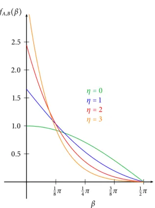
Figure 9. The probability density function fA,B(β)

of intersection angles in dependence on orientation distribution parameterη which varies from 0 to 3.

In Fig. 9 we see that with increasing η the segments at the typical section point show a preferred direction in thez-axis. Since the segment lines tend to have a small polar angleBV for largeη, the segments intersecting S have a small polar angle BA too. For η→0 the probability density function fA,B(β) tends

to cosβ. Note that this is not the isotropic case since for isotropic line-segments it holds fA,B(β) =sin 2β.

MAXIMUM AND MINIMUM RESIDUAL SEGMENT LENGTH

We investigate the stochastic variables M =

max{RA₁,RA₂} and m = min{RA₁,RA₂}, which are only in special cases stochastic independent. We therefore consider first the joint distribution function

FA,m,M(rm,rM) with rm,rM > 0. Furthermore we

consider the marginal distribution functions

FA,M(r) =P(M≤r) =P(RA1 ≤r,R

A

2 ≤r) and

FA,m(r) =P(m≤r) =1−P(RA₁ >r,RA₂ >r)

forr>0. Using simple ideas of probability we obtain

FA,m,M(rm,rM) =

    

   

FA,R₁,R₂(rm,rM)

+FA,R₁,R₂(rM,rm) rm≤rM

−FA,R₁,R₂(rm,rm)

FA,R₁,R₂(rM,rM) rM≤rm

FA,M(r) =FA,R₁,R₂(r,r)

and

FA,m(r) =2FA,R(r)−FA,R₁,R₂(r,r).

With Eqs. 7 and 8 we can relate these distribution functions with the distribution functions ofΨV:

FA,m,M(rm,rM) =

1 ELV

rm Z

0

2FV,L(l+rM)−FV,L(l+rm)−FV,L(l)

dl,

(28)

FA,M(r) =

1 ELV

r

Z

0

FV,L(l+r)−FV,L(l)

dl, (29)

FA,m(r) =

1 ELV

r

Z

0

2−FV,L(l)−FV,L(l+r)

dl. (30)

The marginal distributions simplify withF_V,L(l) =1−

FV,L(l):

FA,M(r) =

1 ELV

r

Z

0

F_V,L(l)−F_V,L(l+r)dl

and

FA,m(r) =

1 ELV

r

Z

0

F_V,L(l) +F_V,L(l+r)dl.

In case of Weibull-distributed lengths it holdsFV,L(l) =

1−e−(ml)k and F_V,L(l) =e−(ml)k. The corresponding results are sketched in Fig. 10.

0.5 1.0

0.5 1.0

l F

F_A,m(l)

FA,M(l)

FV,L(l)

Figure 10. Distribution functions of minimum and maximum residual length, FA,m(l) and FA,M(l), for

ACKNOWLEDGEMENTS

The authors thank K.G. van den Boogaart for inspiring discussion during a seminar at the Institute of Stochastics of the TU Freiberg and U. Hampel, M. Bieberle and S. Boden for providing CT data of fibre-reinforced autoclaved aerated concrete. They are also grateful to the reviewers for series of valuable comments.

REFERENCES

Brandt AM (1985). On the optimal direction of short metal fibres in brittle matrix composites. J Mater Sci 20:3831– 41.

Carling MJ, Williams JG (1990). Fiber length distribution effects on the fracture of short-fiber composites. Polymer Composites 11:307–13.

Chin WK (1988). Effects of fiber length and orientation distribution on the elastic modulus of short fiber reinforced thermoplastics. Polymer Composites 9:27– 35.

Chiu SN, Stoyan D, Kendall WS, Mecke J (2013). Stochastic geometry and its applications. 3rd Ed. Chichester: Wiley.

Fu SY, Lauke B (1996). Effects of fiber length and fiber orientation distributions on the tensile strength of short-fiber-reinforced polymers. Comp Sci Tech 56:1179–90. Hegler RP (1985). Phase separation effects in processing of glass-bead- and glass-fiber-filled thermoplastics by injection molding. Poly Eng Sci 25:395–405.

Kacir L, Narkis N, Ishai O (1975). Oriented short

glass-fiber composites. I. preparation and statistical analysis of aligned fiber mats. Poly Eng Sci 15:525–31.

Li VC, Wang Y, Backer S (1991). A micromechanical model of tension softening and bridging toughening of short random fiber reinforced brittle matrix composites. J Mech Phys Solids 39:607–25.

Maalej M, Li VC, Hashida T (1995). Effect of fibre rupture on tensile properties of short fibre composites. J Eng Mech 121:903–13.

Mecke J, Nagel W (1980). Station¨are r¨aumliche Faserprozesse und ihre Schnittzahlrosen. Elektron Informationsverarb Kyb 16:475–83.

Mecke J, Stoyan D (1980a). A general approach to Buffon’s needle and Wicksell’s corpuscle problem. In: Combinatorial principles in stochastic geometry, Work Collect. Erevan. 164–71.

Mecke J, Stoyan D (1980b). Formulas for stationary planar fibre processes I – general theory. Math Operationsforsch Statist Ser Statist 11:267–79.

Mecke J, Stoyan D (1980c). Stereological problems for spherical particles. Math Nach 96:311–7.

Naaman AE, Reinhardt HW (1996). High performance fiber reinforced cement composites 2 (HPFRCC2). In: Proc 2nd Int RILEM Worksh.

Vaxman A, Narkis M, Siegmann A (1989). Short-fiber-reinforced thermoplastics. Part III: Effect of fiber length on rheological properties and fiber orientation. Polymer Composites 10:454–62.