REGRESSION ANALYSIS WITH LINKED DATA: PROBLEMS
AND POSSIBLE SOLUTIONS.
Andrea Tancredi1
Dipartimento di metodi e Modelli per l’Economia, il territorio e la Finanza, Sapienza Universit`a di Roma, Roma, Italia
Brunero Liseo
Dipartimento di metodi e Modelli per l’Economia, il territorio e la Finanza, Sapienza Universit`a di Roma, Roma, Italia
1. Introduction
From a methodological statistical perspective, the operation of merging two (or more) data sets can be important for two different and complementary reasons:
(i) per s´e, i.e. to obtain a larger reference data set or frame, suitable to perform more accurate statistical analyses;
(ii) to calibrate statistical models via the additional information which could not be extracted from either one of the two single data sets.
If the merging step can be accomplished without errors (maybe because a clear identification key is available and it can be used to match units in different datasets), there are no specific consequences on the statistical procedures under-taken in both the situations. In practice, however, identification keys are rarely available and linkage between statistical records is usually performed under uncer-tainty. This issue has caused a very active line of research among the statistical and the machine learning communities, named “record linkage”, where the possi-bility to make wrong matching decisions must be accounted for, especially when the result of the linking operation, namely the merged data set, must be used for further statistical analyses.
To briefly explain what record linkage is, let us suppose we have two data sets, sayF1and F2, whose records respectively relate to statistical units (e.g. individ-uals, firms, etc.) of partially overlapping samples (or populations), sayS1andS2. Records in each data set consist of several fields, or variables, either quantitative or categorical, which may be observed together with a potential amount of noise. For example, in a file of individuals, fields could besurname, age, sex, and so on.
The goal of a record linkage procedure is to detect all the pairs of units (j, j′), withj∈S1andj′∈S2, such thatjandj′actually refer to the same unit, and this is performed by the use of the information provided by the observed records in the two datasets. If the main goal of the record linkage process is the former outlined above (case (i)), a new data set is created by merging together three different subsets of units: those which are present in both data sets, those belonging to S1 only and those belonging to S2 only. Of course, information regarding the first group of individuals will be richer. Appropriate statistical data analyses may be then performed on the enlarged data set. Since the linkage step is done with uncertainty, the efficiency of the statistical analysis may be jeopardized by i) the presence of duplicate units andii) a loss of power, mainly due to erroneous matching in the merging process.
On the other hand, the latter situation (case (ii)), which is more important for the scope of this paper, is even more challenging, both from a practical and from a methodological perspectives. Let us denote the observed variables in F1 by (Y, V1, V2, . . . , Vh) whereas the observed variables inF2 are (X, V1, V2, . . . , Vh).
One might be interested in performing a linear regression analysis (or any other more complex association model) between Y andX, restricted to those pairs of records which are declared matches after a record linkage analysis based on vari-ables (V1, . . . , Vh). The intrinsic difficulties in such a simple problem are well
documented in Neter et al.(1965) and deeply discussed in Scheuren and Winkler (1993), Scheuren and Winkler (1997) and Lahiri and Larsen (2005). In the re-gression example, it might be easily seen that the presence of false matches (that is, matching record pairs which do not actually refer to the same statistical unit) reduces the observed level of association betweenY andX and, as a consequence, they introduces a bias effect towards zero when estimating the slope of the regres-sion line. Similar biases may appear in every statistical procedure and, in most of the cases, the bias takes a specific direction. As another example, when linkage procedures are used for estimating the sizeN of a population through a capture-recapture approach, the presence of false matches may severely reduce the final estimate ofN.
One should also note, at this point, that in the practical use of record linkage, it is quite usual that the linker (the researcher who matches the two files) and the analyst (the one which performs the statistical analysis) are two different persons, working separately. However, as Scheuren and Winkler (1993) states“... it is important to conceptualize the linkage and analysis steps as part of a single statistical system and to devise appropriate strategies accordingly”.
Following such a suggestion, and putting it into a broader perspective, let us assume we observe variables (Y1, Y2, . . . , Yk, V1, V2, .., Vh) onn1units in fileF1and
variables (X1, X2, . . . , Xp, V1, V2, . . . , Vh) onn2 units in fileF2. In this set-up we
consider the two-fold objective ofi) using the key variablesV1, V2, . . . , Vh to infer
• improve the performance of the linkage step through the use of the extra information contained in the Y’s and X’s. This happens because pairs of records which do not adequately fit the model M will be automatically down-weighted in the matching process;
• allow to account for matching uncertainty in the estimation procedure re-lated to model MinvolvingY’s andX’s.
• improve the accuracy of the estimators of the parameters of model M in terms of bias.
A first attempt to frame the statistical problem of record linkage from a Bayesian perspective can be found in Fortini et al. (2001). In that paper the likelihood function arising from the set of multiple comparisons among different records in the two datasets - comparisons which may involve several different vari-ables - was used to estimate the matching configuration through the use of a specific Markov Chain Monte Carlo (MCMC) technique. That approach, together with the one outlined in Larsen (2005), can be interpreted as a Bayesian alter-native to the classic record linkage approach, formalized by Jaro (1989), which followed the seminal paper by Fellegi and Sunter (1969). Recently, Tancredi and Liseo (2011) have proposed a different Bayesian matching procedure, particularly suited for categorical variables. They explicitly model the fully observed records through a particular measurement error models, inspired by the so called “hit-and-miss” strategy proposed by Copas and Hilton (1990). In the same paper, the problem of uncertainty in population size estimation based on capture-recapture models with linkage uncertainty was discussed in detail. In addition, Liseo and Tancredi (2011) have introduced a record linkage model for continuous data based on a multivariate normal model with measurement error.
regression parameters in a real data example concerning the “end-of life costs”. Another potential limitation of this paper is that the Authors assume a specific matching pattern; in fact, for each singe block of comparisons, all cases in the smaller list are present in the other list.
Practical applications of inference with linked data are very common in bio-statistics and epidemiology. Recent examples include, for instance, Hof and Zwin-derman (2015) who estimated the association between pregnancy duration of the first and second born children from the same mother from a register without mother identifier and Harron et al. (2013) where a data set comprising pedi-atric intensive care admission records has been linked with blood-stream infection surveillance data in order to evaluate the association between this kind of infection and specific risk factors due to pediatric intensive care.
In the next section we will briefly recall the standard approach to record linkage and then we will propose a simplified version of the Bayesian model described in Tancredi and Liseo (2011). We will also provide some details on a possible simulation strategy for the resulting posterior distribution. In Section 3 we will consider a generalization of the method in order to include the regression model. In Sections 4 and 5 we will illustrate our proposals with simulated and real data sets.
2. Record linkage models
In this section we sketch the probabilistic framework for setting up record linkage models. We first introduce the standard model for record linkage and then we discuss a different way of modelling the comparisons among units, which is more amenable to include the inference modelM.
2.1. A brief review of the standard record linkage approach
Suppose we have two matrices of record, sayV1 and V2 of different sizesn1 and n2 respectively. Here
V1= (v11, . . . v1n1) and V2= (v21, . . . , v2n2)
and each singlevij can be represented asvij = (vij1, . . . , vijh), that isVij contains
the observed values of a categorical random vectorv= (v1, . . . , vh) whose support
is
V={vs1s2,...,sh = (s1, . . . , sh) s1= 1. . . , k1;. . .;sh= 1, . . . kh}.
Also, consider the sets M and U of “true matches” and “true non matches” re-spectively. More precisely,
M ={(j, j′) : recordj∈V1 andj′∈V2 refer to the same unit},
and, of course, U =Mc, the complementary set. The main goal of any record
M. The statistical model for a record linkage analysis is built upon the so called comparison vectorsqjj′ = (qjj′1,· · · , qjj′h), where
qjj′l=
{
1 0
v1jl=v2j′l
v1jl̸=v2j′l
, l= 1, . . . , h.
The comparison vectors qjj′ are assumed to be independent and identically
dis-tributed random vectors with a distribution given by the following mixture
p(qjj′|m, u, w) =w h
∏
l=1
mqjj′l
l (1−ml)1−qjj′l+ (1−w)
h
∏
l=1
uqjj′l
l (1−ul)1−qjj′l. (1)
In the previous formula, w represents the marginal probability that a random pair of records belong to the same unit. In other words, w may be interpreted as the percentage of overlapping of the two data sets. The quantities ml andul,
l = 1, . . . , h, are the parameter of the two multinomial distributions associated with the two set of comparisonsM and U, that is
ml= Pr(qjj′l= 1|j, j′ ∈M) ul= Pr(qjj′l= 1|j, j′ ∈U)
Notice that the independence assumption of the comparison vectorsqjj’s is, strictly
speaking, untenable from a probabilistic perspective. Consider the following ex-ample; after comparing record A1 with recordsB1 and B2, and then record A2 with B1 only, the result of the comparison between A2 and B2 is often already known. Also, in the standard model, the key variables are assumed independent of each other. Several extensions of this basic set-up have been proposed, mainly by introducing potential interactions among key variables, see for example Winkler (1995) and Larsen and Rubin (2001).
To test whether a given pair should be allocated toM orU, one may consider either the likelihood ratio
λ= P(qjj′|(j, j
′)∈M)
P(qjj′|(j, j′)∈U)
=
∏h
l=1m
qjj′l
l (1−ml)
1−qjj′l
∏h
l=1u
qjj′l
l (1−ul)1−qjj′l
or - in a Bayesian setting - the posterior probability that a single pair is a match p((j, j′) ∈M|qjj′). In general, a pair of records with a likelihood ratio λ - or a
posterior probability - above a fixed threshold, is declared a match. In practice, the choice of the threshold can be problematic, as illustrated, for example, in Belin and Rubin (1995). In this context, optimization techniques may be helpful to rule out the multiple matches issue, that is the possibility that a single unit in data set A is linked with more than one unit in data set B.
2.2. An alternative Bayesian record linkage model
recordj on data set Vi and let ˜Vi be the corresponding unobserved data matrix.
We assume that
p(V1, V2|V1,˜ V2, γ) =˜ ∏
ijl
p(vijl|v˜ijl, γl) =
∏
ijl
[γlI(vijl= ˜vijl) + (1−γl)q(vijl)].
Notice thatvijl is a mixture of two components, the former is degenerate on the
true value while the latter can be any distribution whose support is the set of all possible values of the variableVl; we believe that - in absence of specific
informa-tion - taking a uniform distribuinforma-tion for the second component of the mixture is a reasonable assumption. This way, q(vijl) = 1/kl. Also notice that, in this new
model, γl is the probability that the variableVl is observed without noise. This
model, known as “hit and miss”, was introduced in the record linkage literature by Copas and Hilton (1990) and recently adapted in the Bayesian framework by Tancredi and Liseo (2011) and Hall et al. (2013); Other examples of finite mix-ture models with uniform background has been discussed in Banfield and Raftery (1993) for clustering continuous data in presence of noise.
To build a model for true values ˜vijlswe need to introduce a matching matrix
C. In particular, let C be a n1×n2 matrix whose unknown entries are either 0 or 1, where Cjj′ = 1 represents a match, Cjj′ = 0 denotes a non-match. We
assume that each data set does not contain replication of the same unit so that
∑
j′Cjj′ ≤ 1, and
∑
jCjj′ ≤ 1. Green and Mardia (2006) have used a similar
matching matrix in slight different context, i.e. in the problem of alignment of unlabelled points for reconstructing molecular shapes. We assume that the joint distribution for ˜V1and ˜V2depends either on the entries of the matching matrixC and on the probability vectorθ= (θs1...sh, s1= 1. . . , k1;. . .;sh= 1. . . , kh) which describes the distribution of the true values one can observe on each sample. More precisely, we assume that
p( ˜V1,V2˜ |C, θ) = ∏
j:Cjj′=0,∀j′
p(˜v1j|θ)
∏
j′:Cjj′=0,∀j
p(˜v2j′|θ)
∏
jj′:Cjj′=1
p(˜v1j,v2˜j′|θ),
(2) where
p(˜vij|θ) =
∏
s1...sh
θs1,...,sI(˜vij=(hs1,...,sh)),
and
p(˜v1j,˜v2j′|θ) =
{
0 if ˜v1j ̸= ˜v2j′ ∏
s1...shθ
I(˜vij=(s1,...,sh))
s1,...,sh if ˜v1j = ˜v2j′
It should be noticed that the above model can be considered a simplified version of the one proposed in Tancredi and Liseo (2011), where an additional layer -introducing a super-population model - was added at the top of the hierarchy. This simplest version, already used in Hallet al.(2013), can be easily obtained by integrating out the additional layer of hierarchy, under specific prior assumptions. Following Hallet al.(2013), we also assume that the key variables are independent. In symbols, settingθl,sl =p(˜vijl=sl|θl), withθl= (θl1, . . . , θl,kl), we assume that
θs1,...,sh =
k
∏
l=1
To complete the model we need to specify a distribution for the matching matrixCand the prior distributions for the parametersγlandθl,l= 1, . . . , h. For
these latter quantities the standard assumptions of independent Beta distributions for the probabilities γl and independent Dirichlet distributions for the vectorsθl
can be adopted. With respect toC, the prior can be elicited in two stages. The first stage consists of a prior distributionp(t),t= 0,1,2, . . . n1∧n2on the random variable T: “number of matched pairs in the two data sets”. At this stage, the researcher can easily collect information, looking at previous experiences or at the statistical characteristics of the data sets (e.g. if the two data sets refer respectively to a census and a sample, we can expect a large number of matched pairs). At the second stage we define a conditional prior distribution for the configuration matrix C giventhe number of matches. We take the natural noninformative choice of a uniform conditional prior on the setC(t)={C:∑
jj′Cj,j′ =t
}
Note also that the
cardinality of C(t) is |C(t)| = (n1 t
)(n2 t
)
t! and that a uniform unconditional prior forC, that will be our choice throughout this paper, can be obtained by assuming p(t)∝ |C(t)|and the aforementioned uniform conditional prior forp(C|T).
2.3. MCMC estimation
The model just outlined cannot be analyzed in a closed form and some form of simulation from the posterior distribution is necessary. In particular, we have implemented a Metropolis within Gibbs algorithm where the updating of param-eters γl and θl can be easily performed by simulating from their respective full
conditional distributions, forl= 1, . . . , h. On the other hand, the updating of the matching matrix C and the true values ˜V1 and ˜V2 is jointly obtained In particu-lar, we propose - via a Metropolis-Hastings step - a new matching matrixC, by adding or deleting one matches or switching two matches. Conditionally on the acceptance of the proposed value for C, a Gibbs step is used for the updating of the elements of ˜V1and ˜V2.
As an example, we illustrate the acceptance probabilities for the specific move in which we “add” a match: when proposing a move fromCjj′ = 0 to Cjj′ = 1,
we accept it with probability
1 ∧ q(C|C
′)
q(C′|C)
p(V1, V2|C′, θ, γ) p(V1, V2|C.θ, γ)
p(C′) p(C),
whereq(C|C′) is the probability of proposing the reversible “deleting match” move, q(C′|C) is the probability of proposing the “adding match” move. Finally,
p(V1, V2|C′, θ, γ) p(V1, V2|C, θ, γ) =
p(v1j, v2j′|θ, γ)
p(v1j|θ, γ)p(v2j′|θ, γ)
= (3)
=
∏h
l=1
(
γ2
lθlv1jlI(v1jl=v2j′l) +γl(1−γl)(θl v1jl+θl v2j′l)/kl+ (1−γl)
2/k2
l
)
∏h
l=1
(
[γlθl v1jl+ (1−γl)/kl][γlθl v2jl+ (1−γl)/kl]
) .
from their full conditional distributions givenCjj′ = 1, that is
p(˜v1jl,˜v2j′l|θ, γ, v1jl, v2j′l, Cjj′ = 1) ∝ θl˜v1jl[γlI(v1jl= ˜v1jl) + (1−γl)/kl]
× [γlI(v2jl= ˜v2jl) + (1−γl)/kl]
if ˜v1jl = ˜v2jl′ and 0 otherwise. Similar expressions can be easily obtained for
the other possible moves, that is deleting a match or switching matches. Notice that the ratio (3), which appears in the above acceptance probability, is the Bayes factor for comparing the hypothesis that the pair (j, j′) is a match versus the alternative hypothesis that it is not a match: see for example Lindley (1977) and Liseo and Tancredi (2011) for similar expressions involving Gaussian distributions. After that a reasonably large sample has been drawn from the posterior distri-bution, we estimate the matching configuration via the following - rather natural - point estimate of the matrixC, namely
b
Cij =
{
1 ifp(Cij = 1|V1, V2)≥12
0 otherwise
Some remarks are necessary here. First, the estimateCbis in some sense suggested by simple decision theoretic considerations (see Tancredi and Liseo (2011)). Notice that, in this situation, the posterior mean cannot be used since it would provide useless real numbers between 0 and 1. Second, the estimated matrix Cb should only be used when the linkage procedure is the final goal of the statistical analysis and a set of potential matches must be declared. If the merged data set is the starting point of a new statistical analysis, then one should try to account for the uncertainty onC provided by the posterior distribution of the matrix itself. This is what we describe next in the particular, although very common, case of linear multiple regression model.
3. Bayesian Regression with linked data
Consider the situation where the first data set is an1×(h+ 1) matrix consisting of the variables (y, V1), and the other data set is a n2×(h+p) matrix, including variables (V2,X) where X= (X1, . . . , Xp). Also, let ˜Xbe the matrix containing
the true (unobserved) covariate values forY. ˜Xhas dimensionn1×p. Condition-ally on ˜Xand on the true matching variables ˜V1 and ˜V2, we assume a Gaussian linear regression model fory, that is,
y|X˜,β, σ2∼N( ˜Xβ, σ2I). (4)
In addition, given the matrices of true values ˜V1 and ˜V2, we assume, for V1 and V2, the “hit and miss” model as illustrated in§2.2.
Conditionally on the matching matrixC, we also assume that the actual covariate values foryjare given by the vectorxj′ (thex-part of thej′-th row of data setB)
only if Cjj′ = 1; otherwise, when the j-th row ofC is a string of 0’s, we assume
that the true covariate values for yj are unknown with a specific distribution
variables. The choice of p(·) is often not crucial and, in general, a multivariate Gaussian distribution will be used. More precisely, we have
p( ˜X|C) = ∏
j,j′:Cjj′=1
δxj′(˜xj)
∏
j:∑j′Cjj′=0
p(˜xj).
For the matrices of true values ˜V1and ˜V2we will adopt the same model described in (2). The posterior simulation can be easily conducted via a Metropolis-Hastings within Gibbs algorithm where the matching matrixC, the true values ˜V1 and ˜V2 and the true covariates ˜Xare jointly updated, in a way very similar to what we have described in the previous section. In particular, in this case, the “add-one-match” move is accepted with probability
1 ∧ q(C|C
′)
q(C′|C)
p(y, V1, V2|C′, θ, γ,β, σ2) p(y, V1, V2|C, θ, γ,β, σ2)
p(C′) p(C), where
p(y, V1, V2|C′, θ, γ,β, σ2) p(y, V1, V2|C, θ, γ,β, σ2)
= ϕ(yj;x
T
j′β, σ2)
∫
ϕ(yj; ˜xTβ, σ2)p(˜x)d˜x
p(v1j, v2j′|θ, γ)
p(v1j|θ, γ)p(v2j′|θ, γ)
, (5)
with ϕ(·;µ, σ2) representing the density of a Normal variable with mean µ and varianceσ2. There are several important remarks and comments concerning the acceptance probability (5).
i) Formula 5 points out that distribution of the matching matrixCis dependent on the values of the β parameters and makes explicit the feed-back effect between the parameters of the regression model and the matching process. This effect has the role to modify the matching estimation leading both to a possible improvement for the record linkage process and to a “bias-correction” effect for the regression estimates.
ii) A closed-form expression for
p(yj;β, σ2) =
∫
ϕ(yj; ˜xTβ, σ2)p(˜x)d˜x
can be obtained, for example, by assuming a multivariate normal forp(˜x). In fact, assuming that ˜x∼N(µ0,Σ0), a simple calculation shows that
yj|β, σ2∼N(µT0β, σ 2+βt
Σ0β).
iii) When the “add-one-match” move is accepted, one updates the true values (˜xj,˜v1j,v˜2j′) by drawing a value from their full conditional distributions
con-ditionally on the new statusCjj′ = 1
Record linkage and regression model
β
0.5 1.0 1.5 2.0 2.5
0
1
2
3
4
5
6
7
Plug−in from the record linkage model
β
0.5 1.0 1.5 2.0 2.5
0
1
2
3
4
5
6
7
Matching uncertainty propagation from the record linkage model
β
0.5 1.0 1.5 2.0 2.5
0
1
2
3
4
5
6
7
Plug−in from the comparison vector record linkage model
β
0.5 1.0 1.5 2.0 2.5
0
1
2
3
4
5
6
7
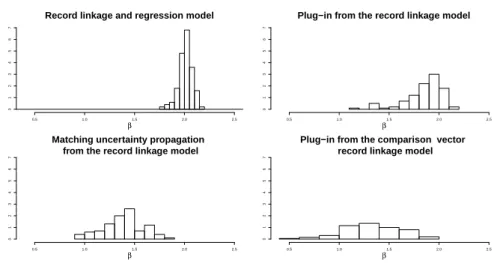
Figure 1 – Simulation study. The posterior distributions of β’s obtained under the “record linkage and regression” model, the “plug-in” approach from the record linkage model, the “matching uncertainty propagation” approach from the record linkage model and the plug-in approach from the “comparison vector record linkage” model (Fortini
et al., 2001). The true value ofβis 2.
4. Simulation study
We now evaluate our hierarchical model for regression analysis with linked data via a simulation study. In particular we have generated 100 pairs of data sets with sizesn1= 100 andn2= 80. The number of true matchesT is Binomial with size 80 and probability 0.75 and the distribution of the matching matrixC givenT is uniform. Each pair of data sets shares 3 independent key variables ˜Vj,j= 1, . . . ,3
with 5, 10 and 50 categories, respectively, and different probability distributions. The probability of correctly observing the true values isγl= 0.95 l= 1, . . . ,3. For
the regression model, we assume a single covariateX whose values are generated from a Normal distribution with mean µx = 100 and variance σ2x = 202 and for
the response variable we assume thaty|xis Normal with meanα+βxwithα= 3 andβ = 2, and varianceσ2
y|x= 10
2.
simulated matching matrix at each MCMC iteration of the record linkage model, are averaged. The resulting estimates ofβ are reported respectively in the upper right and lower left panels of Figure 1. For each simulated pair of data sets we also provide an estimate of the matching matrix via the standard approach outlined in Section 2.1. The lower right panel of Figure 1 shows the corresponding estimates ofβ obtained conditionally on the estimated matching matrix.
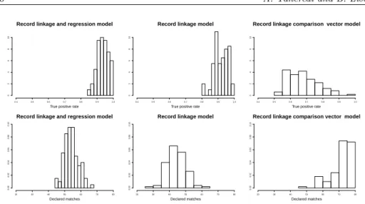
Note that in terms of the inference forβ, the “record linkage and regression” model outperforms all other three estimation strategies. In particular the sam-pling distribution of the estimator E(β|V1, V2, y, X) is centred around the true valueβ= 2 (the observed average is 2.01) while all other estimators are strongly biased towards 0. The bias elimination effect provided by the “record linkage and regression” model is mainly due to the low value of likelihood that the false matches, leading to independent y and xpairs, receive from the regression part of the model. We also notice that the sampling variability ofE(β|V1, V2, y, X) is much smaller when compared with the other approaches. In fact, the introduc-tion of the informaintroduc-tion provided by the linear relaintroduc-tionship between y and x in the “record linkage model” has also had the effect of improving the record link-age quality via a reduction of the matching uncertainty. This feedback effect is confirmed by the true positive matches rate
T P R=
∑
jj′Cjj′Cˆjj′
∑
jj′Cˆjj′
distribution reported in Figure 2 together with the distribution of the declared matches ˆT =∑jj′Cˆjj′. With respect to the other approaches, the “record linkage
and regression” model has, on average, the higher and less variable true positive matches rate and a distribution of ˆT more concentrated on the correct number of matches.
5. An Illustration: Italian Survey of Household Income and Wealth
In this section we illustrate an application of the proposed methods using data from the Italian Survey on Household Income and Wealth. The Italian Survey on Household Income and Wealth (SHIW) is a sample survey conducted by the Bank of Italy every 2 years. The 2010 survey covers 7,951 households composed of 19,836 individuals. Panel households and individuals represent 58% of the data. From the 2010 survey we consider the individual net disposable income as the response variableY of our regression model and the following matching variables: sex, age, marital status, employment status, working sector. From the 2008 survey we consider, in addition to the matching variables, the 2008 net disposable income which is assumed as the covariate X of the regression model. The aim of the application is to calibrate a regression model of Y onX, which is based on those pairs of records which are declared matches by the record linkage procedure.
Record linkage and regression model
True positive rate
0.4 0.5 0.6 0.7 0.8 0.9 1.0
0 2 4 6 8 10
Record linkage model
True positive rate
0.4 0.5 0.6 0.7 0.8 0.9 1.0
0 2 4 6 8 10
Record linkage comparison vector model
True positive rate
0.4 0.5 0.6 0.7 0.8 0.9 1.0
0 2 4 6 8 10
Record linkage and regression model
Declared matches 20 30 40 50 60 70 80
0.00 0.02 0.04 0.06 0.08 0.10
Record linkage model
Declared matches 20 30 40 50 60 70 80
0.00 0.02 0.04 0.06 0.08 0.10
Record linkage comparison vector model
Declared matches 20 30 40 50 60 70 80
0.00 0.02 0.04 0.06 0.08 0.10
Figure 2 – Simulation study. True positive rate and declared matches distributions obtained with the “record linkage and regression” model, the “record linkage only” model and the “comparison vector record linkage” model.
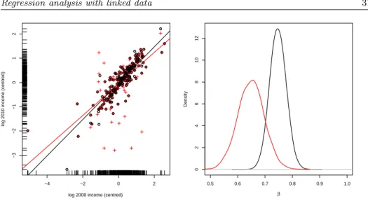
of the true matches and adding 10% of false matches, may lead to dramatically different regression analyses. This is illustrated in Figure 3 for the single block provided by the Friuli region. In the left panel the circle dots represent the true matching configuration while the cross dots represent the perturbed one. In the left panel, the two ordinary least square regression lines, obtained with the two different data sets, are also reported; as expected, the line with the smaller slope refers to the perturbed data set. In the right panel we show the posterior distribu-tions of the slope coefficient with the two data sets and the usual noninformative prior for (α, β, σ). namely π(α, β, σ)∝σ−1. Note that the the two distributions provide quite different credible intervals.
To illustrate the results of our methods we focus on the single Friuli block by comparing different regression analyses. The first one is based on a subset of six key variables for the matching part of the model and the raw income data for the regression fitting. In the upper panels of Figure 4 we show the regression estimates obtained (i) by
i. fitting a Bayesian regression model directly on the true matching configura-tions (203 matches);
ii. applying our regression and matching model;
iii. fitting a Bayesian linear regression via the matching matrix estimated by the record linkage model, i.e. the plug-in approach;
iv. repeating the analysis on the true matching configurations without the two very influential observations with 2008 income level larger than 150000 Euros.
−4 −2 0 2
−3
−2
−1
0
1
2
log 2008 income (centred)
log 2010 income (centred)
0.5 0.6 0.7 0.8 0.9 1.0
0
2
4
6
8
10
12
β
Density
Figure 3 – SHIW data (Friuli block, n1 = 434, n2 = 355). Regression analysis with
the 2010 individual income as the response variable and the 2008 individual income as
a covariate. Left panel: ◦ =true matches, + =declared matches after a perturbation
procedure. Right panel: posterior distributions for the regression coefficientes with the
true matches (black line) and the declared matches.
outliers: since these two observations do not fit the regression model calibrated on the bulk of the matched pairs, they receive a low likelihood of being a match from the regression part of the model. As a consequence they are erroneously considered as non matches, thus removing, or at least mitigating, their effect on the regression estimates. Also, note that the plug-in approach with the record linkage model does not have this protection mechanism against outliers.
In the central panels of Figure 4 we show the results obtained by taking the logarithm of the income variables and repeating the four regression analyses listed above. After the log transformation, the two extreme observations do not produce any effect on the regression fitting: in this case the plug-in approach produces very similar estimates when compared to the true regression line, while the integrated model provides a slightly larger slope coefficient. Finally, in the bottom panels we show all the nine variables and the log-transformed regression variables. With the additional information provided by the three additional key variables the results of the plug-in approach are even more closer to the true fitting.
We conclude this Section by analysing the record linkage performance. In Table 1 we report the false negative rate, FNR, and the false positive rate FPR
F N R=
∑
jj′(1−Cˆjj′)Cjj′
∑
jj′Cjjˆ ′
F P R=
∑
jj′Cˆjj′(1−Cjj′)
∑
jj′Cjjˆ ′
0 50000 100000 150000 200000
0
50000
100000
150000
2008 income (Euros)
2010 income (Euros)
0.4 0.6 0.8 1.0
0
5
10
15
Posterior distributions
β
6 8 10 12
6
7
8
9
10
11
12
2008 log income
2010 log income
0.5 0.6 0.7 0.8 0.9 1.0 1.1
0
5
10
15
Posterior distributions
β
6 8 10 12
6
7
8
9
10
11
12
2008 income (Euros)
2010 income (Euros)
0.4 0.6 0.8 1.0
0
2
4
6
8
10
12
Posterior distributions
β
Figure 4 – Results for the SHIW data (Friuli block). Black line: true regression line
using the 203 true matches. Black dashed line: true regression line without 2 very
TABLE 1
Record linkage performance for the SHIW data with the Friuli block.
model RL RL+REG RL+REG (log) RL RL+REG (log)
key variables 6 6 6 9 9
FNR 0.43 0.33 0.33 0.27 0.22
FPR 0.33 0.30 0.28 0.29 0.30
simple Bayesian matching model. We also note that the record linkage results are affected by the use of the logarithm trasformation for the regression variables which, in this particular example, provide better performance. Such a behaviour is connected with the improved goodness of fit of the linear model on the log vari-ables. As a general comment, one might argue that a perfect linear relationship between the response and the covariates would be practically equivalent to hav-ing a common identification key between the two files. This suggests that strong linear relationships are generally more informative for the matching process than weak relationships. For example, with the above data, the value of theR2 index calculated with the true matches is equal to 0.68 on the original scale and 0.77 after the log trasformations.
6. Discussion
We have described the possibility to deal with record linkage and a regression model for linked data within a common Bayesian framework. The resulting model has the twofold effect of propagating the matching uncertainty into the regression analysis and to account for the information provided by the linear relationships between the response and the covariates into the matching estimation. We have shown via simulated data that the latter effect may significantly improve the estimation process.
References
J. D. Banfield,A. E. Raftery(1993).Model-based gaussian and non-gaussian clustering. Biometrics, pp. 803–821.
T. Belin,D. Rubin(1995).A method for calibrating false - match rates in record linkage. Journal of the American Statistical Association, 90, pp. 694–707.
J. Copas, F. Hilton (1990). Record linkage: statistical models for matching
computer records. Journal of the Royal Statistical Society, A, 153, pp. 287–320.
I. Fellegi,A. Sunter(1969). A theory of record linkage. Journal of the Amer-ican Statistical Association, 64, pp. 1183–1210.
M. Fortini, B. Liseo, A. Nuccitelli,M. Scanu(2001). On Bayesian record
linkage. Research in Official Statistics, 4, pp. 185–198.
H. Goldstein,K. Harron,A. Wade(2012).The analysis of record-linked data
using multiple imputation with data value priors. Statistics in Medicine, 31, no. 28, pp. 3481–3493.
P. J. Green, K. V. Mardia (2006). Bayesian alignment using hierarchical models, with application in protein bioinformatics. Biometrika, 93, pp. 235–254.
R. Gutman,C. C. Afendulis,A. M. Zaslavsky(2013).A Bayesian procedure for file linking to analyze end-of-life medical costs. Journal of the American Statistical Association, 108, no. 501, pp. 34–47.
R. Hall, R. C. Steorts, S. E. Fienberg (2013). Bayesian parametric and
nonparametric inference for multiple record linkage. Working paper, Carnagie Mellon University.
K. Harron, H. Goldstein, A. Wade, B. Muller-Pebody, R. Parslow, R. Gilbert (2013). Linkage, evaluation and analysis of national electronic
healthcare data: application to providing enhanced blood-stream infection surveil-lance in paediatric intensive care. PloS one, 8, no. 12, p. e85278.
M. Hof,A. Zwinderman(2012). Methods for analyzing data from probabilistic
linkage strategies based on partially identifying variables. Statistics in Medicine, 31, no. 30, pp. 4231–4242.
M. Hof, A. Zwinderman (2015). A mixture model for the analysis of data derived from record linkage. Statistics in medicine, 34, no. 1, pp. 74–92.
M. Jaro (1989). Advances in record-linkage methodology as applied to
match-ing the 1985 census of Tampa, Florida. Journal of the American Statistical Association, 84, pp. 414–420.
P. Lahiri, M. D. Larsen(2005). Regression analysis with linked data. Journal of the American Statistical Association, 100, pp. 222–230.
M. Larsen (2005). Advances in record linkage theory: Hierarchical Bayesian record linkage theory. Proceedings of the Section on Survey Research Methods, American Statistical Association, pp. 3277–3283.
M. D. Larsen,D. Rubin(2001).Iterative automated record linkage using mixture models. Journal of the American Statistical Association, 96, pp. 32–41.
D. Lindley (1977). A problem in forensic science. Biometrika, 64, pp. 207–213.
B. Liseo,A. Tancredi(2011).Bayesian estimation of population size via linkage
of multivariate normal data sets. Journal of Official Statistics, 27, pp. 491–505.
J. Neter, E. S. Maynes,R. Ramanathan (1965). The effect of mismatching on the measurement of response errors. Journal of the American Statistical Association, 60, no. 312, pp. 1005–1027.
F. Scheuren,W. E. Winkler(1993). Regression analysis of data files that are
computer matched. Survey Methodology, 19, pp. 39–58.
F. Scheuren,W. E. Winkler(1997). Regression analysis of data files that are
computer matched, Part II. Survey Methodology, 23, pp. 157–165.
A. Tancredi,B. Liseo(2011). A hierarchical Bayesian approach to record
link-age and population size problems. Annals of Applied Statistics, 5, pp. 1553–1585.
W. Winkler(1995). Matching and record linkage. InBuisness Survey Methods, Wiley, New York, pp. 355–384. B. G. Cox, D. A. Binder, B. N. Chinnappa, A. Christianson, M.J. Colledge and P.S. Kott Editors.
Summary
In this paper we have described and extended some recent proposals on a general Bayesian methodology for performing record linkage and making inference using the resulting matched units. In particular, we have framed the record linkage process into a formal statistical model which comprises both the matching variables and the other variables included at the inferential stage. This way, the researcher is able to account for the matching process uncertainty in inferential procedures based on probabilistically linked data, and at the same time, he/she is also able to generate a feedback propagation of the information between the working statistical model and the record linkage stage. We have argued that this feedback effect is both essential to eliminate potential biases that otherwise would characterize the resulting linked data inference, and able to im-prove record linkage performances. The practical implementation of the procedure is based on the use of standard Bayesian computational techniques, such as Markov Chain Monte Carlo algorithms. Although the methodology is quite general, we have restricted our analysis to the popular and important case of multiple linear regression set-up for expository convenience.