The use of radial basis function and non-linear
autoregressive exogenous neural networks to forecast
multi-step ahead of time flood water level
Amrul Faruq a,b,1,*, Shahrum Shah Abdullah b,2, Aminaton Marto c,3, Mohd Anuar Abu Bakar b,4, Shamsul Faisal Mohd Hussein b,5 Che Munira Che Razali b,6
a Department of Electrical Engineering, Faculty of Engineering, Universitas Muhammadiyah Malang, Indonesia b Department of Electronics System and Electrical Engineering, Malaysia-Japan International Institute of Technology, Universiti Teknologi Malaysia, Malaysia
c Department of Environmental Engineering and Green Technology, Malaysia-Japan International Institute of Technology, Universiti Teknologi Malaysia, Malaysia
1[email protected]; 2 [email protected]; 3 [email protected]; 4 [email protected]; 5 [email protected]; 6 [email protected]
* corresponding author
1.
Introduction
Flood disasters continue to occur in many countries around the world and especially in Malaysia. In the recent years river flooding and accompanying landslides, quite frequently occurred in Malaysia, which causes tremendous causalities and properties damage. A sufficiently advanced warning time may save lives and properties by allowing time and effect various structural and another adjustment. Early advanced warning can be achieved through advances in mathematical modeling [1], [2]. A variety of techniques has been developed for flood forecasting which leads to the issue of flood warning system. Artificial intelligence techniques have recently been introduced, including the Artificial Neural Network (ANN) and Support Vector Machine (SVM) [3]. Among these models, ANN has been found suitable for modeling the river flow, flood water level other than rainfall-runoff process. Moreover, ANN is a quick and flexible approach which gives very promising results event with long duration series of time forecasting [4]. A R T I C L E I N F O A B S T R A C T Article history Received October 4, 2018 Revised November 11, 2018 Accepted December 2, 2018 Available online March 21, 2019
Many different Artificial Neural Networks (ANN) models of flood have been developed for forecast updating. However, the model performance, and error prediction in which forecast outputs are adjusted directly based on models calibrated to the time series of differences between observed and forecast values, are very interesting and challenging task. This paper presents an improved lead time flood forecasting using Non-linear Auto Regressive Exogenous Neural Network (NARXNN), which shows better performance in term of forecast precision and produces minimum error compared to neural network method using Radial Basis Function (RBF) in examined 12-hour ahead of time. First, RBF forecasting model was employed to predict the flood water level of Kelantan River at Kuala Krai, Kelantan, Malaysia. The model is tested for 1-hour and 7-hour ahead of time water level at flood location. The same analysis has also been taken by NARXNN method. Then, a non-linear neural network model with exogenous input promoted with enhancing a forecast lead time to 12-hour. Both about the performance comparison has briefly been analyzed. The result verified the precision of error prediction of the presented flood forecasting model.
This is an open access article under the CC–BY-SA license.
Keywords
Floods Forecasting Radial basis function NARX
The design of such a system has been early introduced in [5], three kinds of ANN namely multilayer feedforward neural network (MLFN), Elman partial recurrent neural network (Elman) and time delay neural network (TDNN) as presented suitable for rainfall forecasting in urban catchment. An empirical modelling also called black box modelling has been studied recently in [6], without making many references to physical or hydrological process because this is an event-based modelling and applied in catchment area. Even though the networks could make forecast of rainfall for one step time of 15 minutes ahead. On the other hand, an adaptive-network-based fuzzy inference system (ANFIZ) has been successfully demonstrated by [7] for water level forecasting in the next three hours. Furthermore, an improved flood forecasting fuzzy inference system based Takagi-Sugeno subtractive clustering method has been proposed by [8]. As in [9] provided a fully-online neuro fuzzy model with limited data for flow basin forecasting.
Flood water level forecasting has been presented recently by [10], the feed forward multilayer perceptron (MLP) with Cuckoo search (CS) algorithm model could perform better for 2 hour ahead of time. Recent studies in Malaysia about disaster risk including floods has been discussed by the researchers
[11], [12], [13], [14] and [15]. Studied a predictive and comparative analysis of NARX and Nonlinear Input-Output (NIO) time series prediction has been recently presented by Philip [16]. Some different ANN technique has been discussed over there, and these often addressed for forecasting updating, include error prediction thus far is opened issue in forecasting performance. The performance requirements for the model can also be defined in terms of the requirements at forecasting point, for example, the required accuracy of the forecasts of peak water level, or the lead time provided for surge forecasts. Although there was proposed a flood control and optimization technique to investigate the effects of multiple uncertainties [17]. The proposed method can provide valuable risk information and enable risk-informed decisions with higher reliability.
Unfortunately few studies has been carried out on forecasting performance [18], [19] to meet these requirements. However, these requirements may not always be achievable with the reliable data and models, and this needs to be factored into the overall design. It is officially important that forecasting performance include lead time and error correction is one of the key design criteria, and may dictate the overall design of the model. Despite prior evidence by the researchers [13] and [15], maximum lead time can only adjust for 7 hour and the precise of performance not more than 80%. Hence, the aim of this work is to provide multi-step lead time flood water level forecasting utilizing the upper-river water level station as input employed with NARX and RBF neural network technique. Kelantan River at Kuala Krai, Kelantan, Malaysia was selected as Flood Forecasting Point (FFP) in this work. Both of the performance comparison and output updating error adjustment is also discussed.
2.
Method
Flood water level model and forecast are applied to the Kelantan River catchment as shown in Fig. 1, for predicting flood water level during high flow periods. Kelantan River is located at latitudes 6° 12’ N and longitudes 102° 13’ E. Kelantan River is the main river in Kelantan which occupied 85% of Kota Bharu, state of Kelantan, Malaysia.
It drains a catchment area of about 12,700 km2 in north-east Malaysia including part of the Taman Negara National Park, and flows northwards into the South China Sea with a total population reaches ± 490,000 people in 2010 [20]. The catchment every year receives average 2,900 mm of rainfall due to its subtropical area.
The real-time water level dataset is obtained from the Department of Irrigation and Drainage (DID), Malaysia. These data were collected by their Supervisory Control and Data Acquisition (SCADA) system. These water level include four upper-rivers as shown in Fig. 1 and one FFP considered were collected from January 2011 until January 2012. The real-time water level during flood event data in November 2011 was chosen to evaluate and develop the flood forecast model. Total there were 2880 raw-line data used in 15 minutes time interval. The multi-step ahead of time flood forecasting has been evaluated, and 1 hour, 7 hour and 12 hour lead of time presented in this work.
2.1.Radial Basis Function Neural Networks
Radial Basis Function (RBF) is one of the most popular types in neural network that recently became a powerful function or tool uses for approximation, modeling and forecasting [1], [15], time series prediction [21], RBF as surrogate modeling [22], [23] multi-input multi-output (MIMO) control and optimization [24], [25] and classification problem [26].
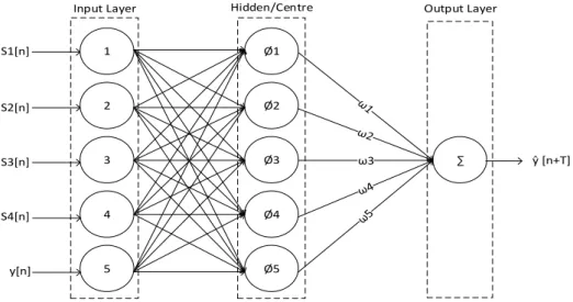
The RBF architecture and their input used in this work as has shown in Fig. 2. The network consists of three layers: an input layer, a hidden layer, and an output layer.
1 2 3 4 Ø1 5 Ø2 Ø4 Ø3 Ø5 ω3 S1[n] S2[n] S3[n] S4[n] y[n]
Input Layer Hidden/Centre Output Layer
ŷ [n+T]
Fig. 2. The RBF neural network forecasting model
Here, R denotes the number of inputs, four upstream-rivers water level and one flood water level at FFP. While Q the number of output, predicted water level of the Kelantan River at the Kuala Krai at time n + T and T will be 1, 7 and 12 hour ahead of time. Equation (1) is used to calculate the output of the RBF NN for Q = 1, the output of the RBFNN in Fig. 2 is calculated according to (1).
1 1
2 1,
S k k kx w
w
x c
where 𝑥 ∈ ℛ𝑅𝑥1 is an input vector, ∅ (. ) is a basis function, || . ||2 denotes the Euclidean norm, 𝑤1𝑘
are the weights in the output layer, S1 is the number of neurons (and centers) in the hidden layer and 𝐶𝑘∈ ℛ𝑅𝑥1 are the RBF centers in the input vector space. Equation (1) can also be written in (2).
x w
,
T( )
x w
where
1
1
1
1
T S Sx
x c
x c
and
11 12 1 1
T Sw
w w
w
The output of the neuron in a hidden layer is a nonlinear function of the distance given by Equation (5).
2 2 / xx
e
where β is the spread parameter of the RBF. For training, the least squares formula was used to find the second layer weights while the centers are set using the available data samples.
In this research, 2880 data were divided into three parts include train datasets, validation datasets, and test datasets. The training datasets were set to 50% simply as 1440 data, and validation data was set to 25% which is 720 data sets, and the remaining also 25% then used for testing data. WL1, WL2, WL3, and WL4 represents the water level in upstream rivers, while y is represented water level at flood location or FFP and
ŷ (𝑛 + 𝑇)
represents predicted flood water level.The training data is the largest data set and used by the neural network to learn pattern present in the data and to fit the parameter. While validation data are used to tune the parameter and validate the network model. Then, for final check of the RBFNN model, testing samples data were used. Here, 720 samples data were evaluated to assess the performance and generalization ability of the network model. Data normalization [27] is done in this work in order to keep the samples data within the same range, noise minimalized, detect trends and flatten the distribution of the variable. These data were scaled between -1 to +1.
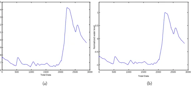
This idea can be illustrated in Fig. 3, it shows the models of actual-observed and normalized data. These sample data were renormalized back to obtain the actual predicted flood water value at the output. The basis function
𝐶
𝑘 is set equal to input vector from training data sets, 5. Then 12 number of spreads is used in the training process. A large spread implies a lot of neurons required to fit a fast-changing function, where a small spread is means less neuron to fit smooth function and the network may not generalized well.(a) (b)
Fig. 3. Flood water level model during high flow periods; (a) actual level and (b) Normalize-based data.
2.2.Nonlinear Autoregressive Exogenous Neural Networks
The NARX neural network is derived from a class of discrete-time nonlinear systems, i.e., the non-linear autoregressive with exogenous input (NARX) models [28]. The model is used to perform a multi-step ahead flood forecasting in this work, which includes 1 hour, 7 hour and 12 hour lead of time. Actual
0 500 1000 1500 2000 2500 3000 16 17 18 19 20 21 22 23 24 25 Total Data W a te r L e ve l (m ) 0 500 1000 1500 2000 2500 3000 -1 -0.5 0 0.5 1 Total Data N o rm a li ze d w a te r le ve l
model of flood at FFP is chosen as exogenous variable in the neural network model. The mathematical form of the NARX feed-forward is defined by the expression in (6).
𝑦 (𝑡) = 𝑓(𝑦(𝑡 − 1), 𝑦(𝑡 − 2), … , 𝑦(𝑡 − 𝑛𝑦),
𝑢(𝑡 − 1), 𝑢(𝑡 − 2), … , 𝑢(𝑡 − 𝑛𝑢)
Where
𝑢 (𝑡)
and𝑦 (𝑡)
represent the inputs and outputs, respectively, of the network at a discrete time step t;𝑛
𝑢 and𝑛
𝑦 are the input and output layers, respectively, of the network; and𝑓
is a nonlinear function that is generally unknown and can be approximated by the common feedforward network. The outputs𝑦 (𝑡)
are regressed onto previous values of the independent or exogenous input signal, improving the convergence time of the network. Each neuron produces an output that is fed back into the hidden node, which transforms the non-linear variables into an output that learns the time series behavior [28], [29].A total of 2880 data were partitioned into two parts; the first 75% and 25% respectively used for training and testing the network. These input series and output series respectively of flood water level can be expressed in vector matrix (7) and (8). In which, WL1 (1) represents first water level data in upstream river 1 until last (2880) water level data in upstream river 1, river 2, river 3, and river 4. And then one flood river location as Flood Forecasting Point (FFP).
Input series = { [ 𝑊𝐿1 (1); 𝑊𝐿2 (1); 𝑊𝐿3 (1); 𝑊𝐿4 (1) ] [ 𝑊𝐿1 (2); 𝑊𝐿2 (2); 𝑊𝐿3 (2); 𝑊𝐿4 (2) ] [ 𝑊𝐿1 (3); 𝑊𝐿2 (3); 𝑊𝐿3 (3); 𝑊𝐿4 (3) ] … [ 𝑊𝐿1 (2880); 𝑊𝐿2 (2880); 𝑊𝐿3 (2880); 𝑊𝐿4 (2880) ]} Output series = [ 𝐹𝐹𝑃(1) 𝐹𝐹𝑃(2) 𝐹𝐹𝑃(3) … 𝐹𝐹𝑃(2880) ] (8)
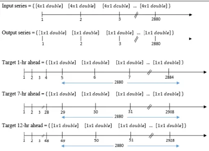
To represent 1hr, 7hr and 12hr lead of time, a new set of 75% inputs [(N+T)x4] and 25% [(N+T)x1] validation output is provided in order to perform multi-step-ahead prediction. These inputs are used for doing the forecasting process and validated how good the network was performing by plotting the forecasting result with the real outputs of T ahead of time. To begin this process, the input and output vector matrices as constructing in Fig. 4.
Fig. 4. The input and target data vector matrices used in NARX technique
A normalization function was applied between -1 to +1 as the same analysis in RBF approach. In this work, a Levenberg-Marquardt (LM) training function [30] chosen in order to optimize the solution. The NARXNN architecture with 4 input series and 1 output series respectively represent for 4 upstream
rivers water level and 1 water level in the downstream river, as illustrated in Fig. 5. The flood water level forecast using NARX algorithm as follows: (1) first, read input data which is water level in four upstream rivers and one water river in flood location; (2) defining input and output, four input data and one predicted output data; (3) partitioning training and testing data; (4) train data using Levenberg-Marquardt backpropagation technique then saved the trained neural network model; and (5) predict time-step ahead output as test data using trained data.
1 2 3 4 Ø1 Ø2 Ø3 Ø10 S1[n] S2[n] S3[n] S4[n]
Input Layer Hidden Neurons Output Layer
ŷ [n+T] ω3
1:X
1:X
Delay Time
Fig. 5. Closed-loop NARX Neural Network model
3.
Results and Discussion
The performance of RBF and NARX network model was evaluated using Root Mean Square Error (RMSE) to measure the differences between estimated river water river output,
ŷ (𝑛 + 𝑇)
and actual reference river water level,𝑦
. It is stated in (9). In order to validate how the networks was performing, by evaluating the regression value of forecasted model and the actual water level. The value of best fit is calculated according to Equation (10).𝑅𝑀𝑆𝐸 = √1 𝑁∑ (𝐸𝑖− 𝑅𝑖) 2 𝑁 𝑖=1 𝐵𝑒𝑠𝑡 𝐹𝑖𝑡 = 100 𝑥 ( 1−𝑛𝑜𝑟𝑚 (𝑦̂[𝑛+𝑇]−𝑦[𝑛+𝑇]) 𝑛𝑜𝑟𝑚 (𝑦[𝑛+𝑇]−𝑚𝑒𝑎𝑛 (𝑦[𝑛+𝑇])))
where,
𝐸
𝑖 is the estimated variable or predicted flood water level,ŷ (𝑛 + 𝑇)
.𝑅
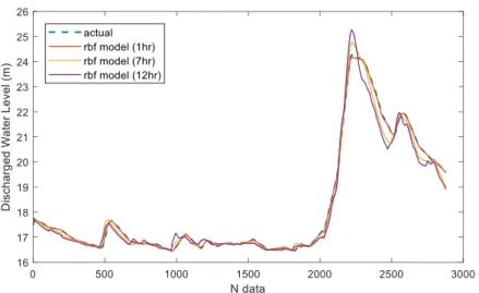
𝑖 is the reference variable or measured water level model, y and N is the total of number of data. It is shown in Fig. 6 that RBFNN-trained data is used to perform the simulation for 720 validation data.To ensure the accurate of the model, 720 data then tested. Unlike RBFNN model, 75% raw-line datasets were examined for training process in NARX model. These trained data then employed to 25% datasets for testing process. Result of forecasted model using NARX network as shown in Fig. 7. While Table 1 shows the performance evaluation and its parameters used in this work. The NARX neural network model has shown remarkable achievements in this work.
Fig. 7. Multi-step T hour ahead of NARX model and actual Table 1. Flood water level forecasting performance result
Algorithm T ahead (hr) NumCenter ValSpread RMSE BestFit Regression
1 5 12 0.0091 98.12% 0.99983
RBF-NN 7 5 12 0.0891 85.35% 0.99005
12 5 12 0.1439 76.95% 0.97518
T ahead (hr) NumCenter TapedDelay RMSE BestFit Regression
1 10 2 0.0746 87.19% 0.99231
NARX-NN 7 10 2 0.0842 85.56% 0.98963
12 10 2 0.1154 80.23% 0.98358
According to Table 1, it is can be analyzed that RBF-NN technique able to produce good performance indicated by error value and best fit evaluation in examined 1-hour ahead of time. Unlike the RBF-NN however, NARX network shows better performance compare with RBF network in term of forecasting accuracy and error distribution respectively in examined 7-hour and 12-hour ahead of time. Using the default NARX network as 10 neurons and taped delay line is 2, this network able to produce 0.1154 RMSE with the best fit 80.23% for 12-hour lead of time flood forecasting. While RBF-NN can approach the best fit value 76.95%. The results of the correlational analysis are summarized in Fig. 8.
It is also can be observed that the best fit of this network still performs better for more than 80% in multi-step ahead of time. In this case, it indicates that the use of NARX network for flood water level forecasting provides the most accurate prediction with an error 0.0842 and 0.1154 for 7-hour and 12-hour time ahead respectively to the actual flood model. However, the RBF network promises a simple network structure and elapsed time needed for examining the flood forecasting model. With a constant number of neuron and spread value, the RBF network performs with best fit more than 75% precision to the actual flood model for 12-hour ahead of time.
4.
Conclusion
The suitable of non-linear autoregressive networks model with exogenous input in short-term flood water level forecasting has been examined in this research. Since the performance of flood forecasting model, include the forecasting precision is still in opened issue. Additionally, the radial basis function neural network employed in order to compare the reasonably good performance of flood forecasting model. Even though performance RBF model fall behind with NARX in term of multi-step lead of time forecasting, the RBF network configuration promises a simply model and smaller. Unlike the RBF model, NARX shows better performance even for forecasts a multi-step time ahead of flood water level. The NARX relatively produce minimum error with 80% highly best fit approximation in examined 12-hour ahead of time forecasting. Furthermore, numerous input variables such as rainfall-runoff information, wind speed and stream flow of catchment can be considered for future work in advance. Exploring more possible parameters setting will make the network to learn the pattern movement of the numerous data. This makes sense to build a robustness of forecasting model.
Acknowledgment
The authors wish to express their sincerest gratitude to the Malaysia-Japan International Institute of Technology, Universiti Teknologi Malaysia for supporting and providing the facilities of this research. The Department of Irrigation and Drainage, Malaysia for providing the observed flood water level data. And The Universitas Muhammadiyah Malang for supporting this study.
References
[1] Fi-John Chang, J.-M. Liang, and Y.-C. Chen, “Flood Forecasting Using Radial Basis Function Neural Networks,” IEEE Trans. Syst. Man. Cybern., vol. 31, no. 4, pp. 530–535, 2001, doi: 10.1109/5326.983936. [2] A. Y. Shamseldin and K. M. O’Connor, “A non-linear neural network technique for updating of river flow
forecasts,” Hydrol. Earth Syst. Sci. Discuss., vol. 5, no. 4, pp. 577–598, 2001, doi: 10.5194/hess-5-577-2001. [3] L. Lu and S. Zhang, “Short-term Water Level Prediction using Different Artificial Intelligent Models,” in
2016 Fifth International Conference on Agro-Geoinformatics (Agro-Geoinformatics), 2009, doi:
10.1109/Agro-Geoinformatics.2016.7577678.
[4] J. Abbot and J. Marohasy, “Skilful rainfall forecasts from artificial neural networks with long duration series and single-month optimization,” Atmos. Res., vol. 197, no. July, pp. 289–299, 2017, doi: 10.1016/j.atmosres. 2017.07.015.
[5] K. C. Luk, J. E. Ball, and A. Sharma, “An application of artificial neural networks for rainfall forecasting,”
Math. Comput. Model., vol. 33, no. 6, pp. 683–693, 2001, doi: 10.1016/S0895-7177(00)00272-7.
[6] C. L. Jun, Z. S. Mohamed, A. L. S. Peik, S. F. M. Razali, and S. Sharil, “Flood forecasting model using empirical method for a small catchment area,” J. Eng. Sci. Technol., vol. 11, no. 5, pp. 666–672, 2016, available at: Google Scholar.
[7] F. J. Chang and Y. T. Chang, “Adaptive neuro-fuzzy inference system for prediction of water level in reservoir,” Adv. Water Resour., vol. 29, no. 1, pp. 1–10, 2006, doi: 10.1016/j.advwatres.2005.04.015. [8] A. K. Lohani, N. K. Goel, and K. K. S. Bhatia, “Improving real time flood forecasting using fuzzy inference
system,” J. Hydrol., vol. 509, pp. 25–41, 2014, doi: 10.1016/j.jhydrol.2013.11.021.
[9] M. Ashrafi, L. H. C. Chua, C. Quek, and X. Qin, “A fully-online Neuro-Fuzzy model for flow forecasting in basins with limited data,” J. Hydrol., vol. 545, pp. 424–435, 2017, doi: 10.1016/j.jhydrol.2016.11.057.
[10] S. Phitakwinai, S. Auephanwiriyakul, and N. Theera-Umpon, “Multilayer perceptron with Cuckoo search in water level prediction for flood forecasting,” Proc. 2016 Int. Jt. Conf. Neural Networks, vol. 2016–Octob, no. 1, pp. 519–524, 2016, doi: 10.1109/IJCNN.2016.7727243.
[11] N. W. Chan, “Impacts of disasters and disasters risk management in Malaysia: The case of floods,” Econ.
Welf. Impacts Disasters East Asia Policy Responses., no. December, pp. 503–551, 2012, doi:
10.1007/978-4-431-55022-8_12.
[12] M. S. Bin Khalid and S. B. Shafiai, “Flood Disaster Management in Malaysia: An Evaluation of the Effectiveness Flood Delivery System,” Int. J. Soc. Sci. Humanit., vol. 5, no. 4, pp. 398–402, 2015, doi: 10.7763/IJSSH.2015.V5.488.
[13] F. A. Ruslan, A. M. Samad, M. Tajjudin, and R. Adnan, “7 hours flood prediction modelling using NNARX structure: Case study Terengganu,” Proceeding - 2016 IEEE 12th Int. Colloq. Signal Process. its Appl. CSPA
2016, no. November, pp. 263–268, 2016, doi: 10.1109/CSPA.2016.7515843.
[14] S. Shafiai and M. S. Khalid, “Flood Disaster Management in Malaysia: A Review of Issues of Flood Disaster Relief during and Post-Disaster,” Int. Soft Sci. Conf., no. 1983, pp. 1–8, 2016, doi: 10.15405/epsbs. 2016.08.24.
[15] Abu Bakar, M.A, Abdul Aziz F.A., Mohd Hussein S.F., Abdullah S.S., Ahmad F. “Flood Water Level Modeling and Prediction Using Radial Basis Function Neural Network: Case Study Kedah,” Model. Des.
Simul. Syst. AsiaSim, vol. 751, pp. 225–234, 2017, doi: 10.1007/978-981-10-6463-0_20.
[16] O. O. Philip and B. T. Adeleke, “Predictive and Comparative Analysis of NARX and NIO Time Series Prediction,” Am. J. Eng. Res., vol. 6, no. 9, pp. 155–165, 2017, available at: http://www.ajer.org/papers/ v6(09)/T0609155165.pdf.
[17] F. Zhu, P. A. Zhong, Y. Sun, and W. W. G. Yeh, “Real-Time Optimal Flood Control Decision Making and Risk Propagation Under Multiple Uncertainties,” Water Resour. Res., vol. 53, no. 12, pp. 10635–10654, 2017, doi: 10.1002/2017WR021480.
[18] W. K. Lee and T. A. Tuan Resdi, “Simultaneous hydrological prediction at multiple gauging stations using the NARX network for Kemaman catchment, Terengganu, Malaysia,” Hydrol. Sci. J., vol. 61, no. 16, pp. 2930–2945, 2016, doi: 10.1080/02626667.2016.1174333.
[19] A. Wibowo, S. H. Arbain, and N. Z. Abidin, “Combined multiple neural networks and genetic algorithm with missing data treatment: Case study of water level forecasting in Dungun River - Malaysia,” IAENG
Int. J. Comput. Sci., vol. 45, no. 2, 2018, available at: http://www.iaeng.org/IJCS/issues_v45/issue_2/
IJCS_45_2_03.pdf.
[20] Department of Information, Ministry of Communications and Multimedia, “Population by States and Ethnic Group,” Malaysia, 2017, available at: https://www.mcmc.gov.my/skmmgovmy/media/General/pdf/
MCMC-Internet-Users-Survey-2017.pdf.
[21] H. Haviluddin and A. Jawahir, “Comparing of ARIMA and RBFNN for short-term forecasting,” Int. J. Adv.
Intell. Informatics, vol. 1, no. 1, pp. 15–22, 2015, doi: 10.26555/ijain.v1i1.10.
[22] M. F. N. Shah, S. S. Abdullah, and A. Faruq, “Multi-objective optimization of mimo control system using surrogate modeling,” in IEEE International Conference on Control System, Computing and Engineering, 2011, pp. 138–143, doi: 10.1109/ICCSCE.2011.6190511.
[23] A. Faruq, S. S. Abdullah, M. Fauzi, and S. Nor, “Optimization of depth control for Unmanned Underwater Vehicle using surrogate modeling technique,” in 2011 4th International Conference on Modeling, Simulation
and Applied Optimization, ICMSAO 2011, 2011, doi: 10.1109/ICMSAO.2011.5775543.
[24] M. F. N. Shah, M. A. Zainal, A. Faruq, and S. S. Abdullah, “Metamodeling approach for PID controller optimization in an evaporator process,” in 2011 4th International Conference on Modeling, Simulation and
Applied Optimization, ICMSAO 2011, 2011, doi: 10.1109/ICMSAO.2011.5775616.
[25] A. Faruq, M. F. N. Shah, and S. S. Abdullah, “Multi-objective optimization of PID controller using pareto-based surrogate modeling algorithm for MIMO evaporator system,” Int. J. Electr. Comput. Eng., vol. 8, no. 1, pp. 556–565, 2018, doi: 10.11591/ijece.v8i1.pp556-565.
[26] J. Tian, M. Li, F. Chen, and N. Feng, “Learning Subspace-Based RBFNN Using Coevolutionary Algorithm for Complex Classification Tasks,” IEEE Trans. Neural Networks Learn. Syst., vol. 27, no. 1, pp. 47–61, 2016, doi: 10.1109/TNNLS.2015.2411615.
[27] W. Yan, “Toward automatic time-series forecasting using neural networks,” IEEE Trans. Neural Networks
Learn. Syst., vol. 23, no. 7, pp. 1028–1039, 2012, doi: 10.1109/TNNLS.2012.2198074.
[28] H. Xie, H. A. O. Tang, and Y. Liao, “Time Series Prediction Based On Narx Neural Networks : An Advanced Approach,” in Proceedings of the Eighth International Conference on Machine Learning and
Cybernetics, 2009, no. July, pp. 12–15, doi: 10.1109/ICMLC.2009.5212326.
[29] I. M. Yassin, M. F. A. Khalid, S. H. Herman, I. Pasya, N. A. Wahab, and Z. Awang, “Multi-Layer Perceptron (MLP)-Based Nonlinear Auto-Regressive with Exogenous Inputs (NARX) Stock Forecasting Model,” Int. J. Adv. Sci. Eng. Inf. Technol., vol. 7, no. 3, pp. 1098–1103, 2017, doi: 10.18517/ijaseit.7.3.1363. [30] S. M. Guzman, J. O. Paz, and M. L. M. Tagert, “The Use of NARX Neural Networks to Forecast Daily Groundwater Levels,” Water Resour. Manag., vol. 31, no. 5, pp. 1591–1603, 2017, doi: 10.1007/s11269-017-1598-5.