COPYRIGHT NOTICE
FedUni ResearchOnline
http://researchonline.ballarat.edu.au
This is the submitted for peer-review version of the following article:
Morales-Silva, D., & Gao, D.
(2013). Complete solutions and triality theory to a
nonconvex optimization problem with double-well potential in R
n.
Numerical
Algebra, Control and Optimization, 3(2). 271-282
© American Institute of Mathematical Sciences.
This is the author’s version of the work. It is posted here with permission
of the publisher for your personal use. No further distribution is permitted.
Complete Solutions and Triality Theory to a
Nonconvex Optimization Problem with Double-Well
Potential in
IR
nDaniel M. Morales Silva, David Y. Gao∗ School of Science, Information Technology and Engineering,
University of Ballarat, Mt Helen, VIC 3350, Australia
Abstract
The main purpose of this research note is to show that the triality theory can always be used to identify both global minimizer and the biggest local maximizer in global optimization. An open problem left on the double-min duality is solved for a nonconvex optimization problem with double-well potential inIRn, which leads to a complete set of analytical solutions. Also a convergency theorem is proved for linear perturbation canonical dual method, which can be used for solving global optimization problems with multiple solutions. The methods and results presented in this note pave the way towards the proof of the triality theory in general cases.
Keywords: Canonical duality theory, Triality, Double-well potential, Global optimization, Nonlinear algebraic equations, Perturbation.
1. Primal Problem and Motivation
We are interested in analytical solutions to the following global minimization problem ((P) in short):
(P) : min{Π(x) =W(x)− hx, fi | x∈IRn}, (1)
∗Corresponding author
Email addresses: [email protected](Daniel M. Morales Silva ),
wheref ∈IRn is a given vector,hx, firepresents the inner product inIRn, and W :IRn→IRis a fourth order polynomial of the form
W(x) := α 2 1 2|x| 2 −λ 2 ,
in which,αandλare given positive parameters.
-2 0 2 4 6 -4 -3 -2 -1 0 1 2 3 4 0.5*(0.5*x 2-3) 2-x x
(a) Function Π whenn, f, α= 1 and
λ= 3. -4 -3 -2 -1 0 1 2 3 4 -4 -3-2 -1 0 1 2 3 4 0 0.5 1 1.5 2 2.5 3 3.5 4 4.5 z z=0.5(0.5(x2 +y2 )-3)2 x y z (b) Function Π whenn= 2, f = 0, α= 1 andλ= 3. Figure 1: Graphs of Π(x)
The non-convex problem (P) appears extensively in many applications of sciences and engineering. For example, in the case thatn= 1, Π(x) is a double-well function(see figure 1a), which was first studied by van der Waals in thermal mechanics in 1895. Ifn= 2 andf = 0 this is the so-called Mexican hat function (see Figure 1b) in cosmology and theoretical physics. Due to the nonconvex-ity, the function Π(x) may possess multiple critical points, determined by the necessary condition ∇Π(x) =α 1 2|x| 2 −λ x−f = 0.
Direct methods for solving this nonlinear algebraic equation are difficult, and to identify the global minimizer is a main task in global optimization.
If instead of the functionW considered above, we were to consider the func-tionWB :IRn →IRdefined by WB(x) := α 2 1 2|Bx| 2 −λ 2 ,
whereB:IRn →IRm is a linear transformation (not identically zero), now the function Π(x) =WB(x)− hf, xigives a more general case for problem (P). Yet,
if we take f ∈ R(BtB), we can always reduce (P) to the case where B = I
in the following way: make y =Bx and letf =B(BtB)†f, where (BtB)† is
the Moore-Penrose pseudoinverse ofBtB (see [2], [12] and references therein).
Notice that sincef ∈R(BtB) thenBtf =f and
hf, xi=hBtf , xi=hf , Bxi=hf , yi. With this, we can define the function ΠB:R(B)→IRwhere
ΠB(y) = α 2 1 2|y| 2 −λ 2 − hf , yi.
If y0 ∈ R(B) is a solution of ΠB, there must exist a x0 ∈ IRn such that
Bx0=y0, then
BtBx0=Bty0
and from this, we can takex0 = (BtB)†Bty0 as a solution for Π. Thanks to
this, we will study only the case whenB=I.
Canonical duality theory developed in [3] is potentially powerful for solving a large class of nonconvex/nonsmooth/discrete problems in both analysis and global optimization [7, 8, 9]. This theory is composed mainly of (a) a canoni-cal dual transformation, (b) a complementary-dual principle, and (c) a triality theory. It was shown in [4] that by the canonical dual transformation, the fourth-order nonconvex problem (P) is equivalent to an one-dimensional canon-ical dual problem which can be solved analytcanon-ically to obtain all critcanon-ical points. The complementary-dual principle shows that a complete set of solutions to the primal problem can be represented analytically by these canonical dual solu-tions. By the triality theory, both global minimizer and local maximizer can be identified. However, it was discovered in 2003 that in order to identify local minimizer, the triality theory proposed in [3] needs “certain additional con-straints” (see Remark 1 in [4]). Therefore, the double-min duality statement in this triality theory was left as an open problem in global optimization [5].
The canonical duality theory and the associated triality have been challenged recently by Voisei and Z˘alinescua in a set of more than seven papers1.
Unfortu-nately, in these papers, they either made mistakes in understanding some basic terminologies of finite deformation mechanics, or repeatedly address the same type of open problem for the double-min duality left unaddressed by Gao in [4, 5]. For example, theexternal energyF(u) in conservative systems (the case studied by Gao and Strang in [10]) means that the gradient∇F(u) must be a given external force field. Therefore, the function(al)F(u) in Gao and Strang’s work can not be quadratic. However, in their paper published recently in Ap-plicable Analysis, quadratic F(u) has been used by Voisei and Z˘alinescua in all “counterexamples”. Also, interested readers should find that the references [4, 5], where the open problem was remarked, never been cited in any one of their papers.
The main purpose of this paper is to solve this open problem such that the proposed problem (P) can be solved completely. The method and results presented in this paper have been used to prove the triality theory for global optimization problems with general polynomials [11] and general objective func-tions [13, 15].
2. Canonical Dual Problem and Analytical Solutions
Following the standard procedure of the canonical dual transformation, first we need to choose a geometric operator Λ : IRn → [−λ,+∞) given by the following function
Λ(x) = 1 2|x|
2
−λ,
and the associated canonical functionV : [−λ,+∞)→IR+ defined by
V(ξ) = α 2ξ
2.
Therefore, the primal function Π can be reformulated as
Π(x) =V(Λ(x))− hf, xi.
1See the web page at http://www.math.uaic.ro/
By the Legendre transformation (see [1, 17, 19]), the conjugate function Vc: [−αλ,+∞)→IR + is given by Vc(ς) = ς 2 2α.
With this, the Gao-Strangtotal complementary functionΞ :IRn×[−αλ,+∞)→
IR, associated to the problem (P) can be defined as follows: Ξ(x, ς) =ςΛ(x)− ς
2
2α− hf, xi.
Via this Ξ(x, ς), the canonical dual function Πd: [−αλ,+∞)→IRcan be finally
obtained by [4] Πd(ς) := sta x∈IRnΞ(x, ς) ={Ξ(x0, ς)| ∇xΞ(x0, ς) = 0} = −|f| 2 2ς − ς2 2α−ςλ, ∀ς ∈[−αλ,+∞),
where the notation sta{∗}stands for finding stationary points of the function given in{∗}.
Notice that if ς >0 then the dual function Πd(ς) is strictly concave which
admits a unique global maximizer; however, Πd(ς) is a d.c. function (difference
of convex functions) on [−αλ,0), which should give us information about local extrema of the primal function Π. Therefore, the canonical dual problem is proposed in the following stationary form:
(Pd) : sta
ς∈[−αλ,+∞)Π
d(ς) =
{Πd(ςo)|∇Πd(ςo) = 0}. (2)
By the fact that the canonical dual problem (Pd) has only one variable, the
criticality condition∇Πd(ς) = 0, where
∇Πd(ς) = |f|
2
2ς2 −
ς
α−λ, (3)
leads to a quebec algebraic equation
2ς2ς α+λ
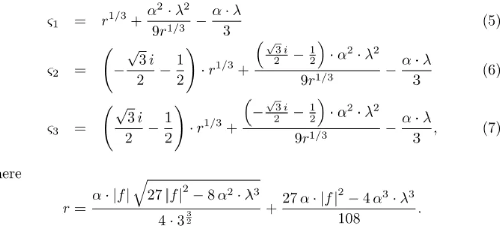
which can be solved explicitly to obtain all three possible real solutions: ς1 = r1/3+α 2·λ2 9r1/3 − α·λ 3 (5) ς2 = − √ 3i 2 − 1 2 ! ·r1/3+ √ 3i 2 − 1 2 ·α2·λ2 9r1/3 − α·λ 3 (6) ς3 = √ 3i 2 − 1 2 ! ·r1/3+ −√23i − 1 2 ·α2·λ2 9r1/3 − α·λ 3 , (7) where r=α· |f| q 27|f|2−8α2·λ3 4·332 +27α· |f| 2 −4α3·λ3 108 .
It is not difficult to show that if |f|2 > 8α2λ3/27 then ς1 is the only real
positive root and if|f|2= 8α2λ3/27 thenς1 is positive, andς2=ς3=−2αλ/3.
If 0<|f|2<8α2λ3/27, equations (5)-(7) can be simplified further to obtain:
ς1 = αλ 3 2 cos 1 3cos −127|f|2 4α2λ3 −1 −1 (8) ς2 = αλ 3 2 cos 1 3cos −1 27|f|2 4α2λ3 −1 +4π 3 −1 (9) ς3 = αλ 3 2 cos 1 3cos− 127|f|2 4α2λ3 −1 +2π 3 −1 . (10)
Moreover, we will have thatς1>0> ς2>−2αλ/3> ς3>−αλ.
-15 -10 -5 0 5 10 15 -4 -3 -2 -1 0 1 2 3 4 2*x 2*(x+3) x
Theorem 1 (Analytical Solutions [4]). Let f ∈ IRn\ {0} and {ςi} be the
real roots of Equation (4). Then, xi = f /ςi are stationary points of (P) for
everyi andΠ(xi) = Πd(ςi).
Proof: Notice that Λ(xi) =ςi/α, we have
Λ(xi) = 1 2|xi| 2 −λ= |f| 2 2ς2 i −λ
but sinceςi is solution of (4), we have
Λ(xi) = ςi α +λ −λ= ςi α. (11)
Now, if we differentiate the function Π we will have
∇Π(x) =αΛ(x)x−f (12) and so ∇Π(xi) =αΛ(xi)xi−f =α· ςi α · f ςi − f = 0. On the other hand
Π(xi) =α 2 · ς2 i α2 − |f|2 ςi = ς2 i 2α− 2ς2 i α + 2ςiλ =−3ς 2 i 2α −2ςiλ and Πd(ς i) =−| f|2 2ςi − ς2 i 2α−ςiλ=− ς2 i α +ςiλ − ς 2 i 2α−ςiλ=− 3ς2 i 2α −2ςiλ, so we have Π(xi) = Πd(ςi) as expected.
Theorem 1 shows that the stationary points of the dual problem induce naturally stationary points of the primal with zero duality gap. Using (12), it can be seen that if any stationary point of Π exists, it must be in the same direction off. Therefore, by analyzing the functionW(rf) withr∈IRit can be seen that the possible stationary points ofW(rf) satisfy the following equation:
αr r2 2 |f| 2−λ = 1. (13)
Sincef 6= 0, then r 6= 0 and by substitutingr= 1/ς in (13) we will have (4). Thus, problem (P) has at most three critical points. In the next section, we will show that the extremality of these solutions can be identified by a refined triality theory.
3. Triality Theory and Perturbation
The following spaces are important for understanding the triality theory:
X♯ := x∈IRn| hf, xi |f||x| < r −2ς ς2 2+ 2αλ , (14) X♭ := x∈IRn| hf, xi |f||x| > r − ς2 2ς2+ 2αλ . (15)
Theorem 2 (Refined Triality Theory). Let f ∈IRn be a given vector such
that 0<|f|2 <8α2λ3/27,{ς
i} with i= 1,2,3 the three real roots of Equation
(4) such thatς1 >0 > ς2 >−2αλ/3 > ς3 >−αλ and let xi =f /ςi. Then we
have
i) x1 is a global minimizer ofΠ,ς1 is a maximizer of Πd in (0,+∞), and
Π(x1) = min
x∈IRnΠ(x) =ς max
∈(0,+∞)Π
d(ς) = Πd(ς
1). (16)
ii) There existXo andIoneighborhoods of x3 andς3 respectively such thatx3 is a local maximizer ofΠ(x)inXoandς3 is a local maximizer ofΠd(ς)in
Io, and Π(x3) = max x∈Xo Π(x) = max ς∈Io Πd(ς) = Πd(ς3). (17)
iii) There existsI1 a neighborhood of ς2 such that ς2 is a local minimizer of
Πd(ς) in I
1 and x2 is a saddle point of Π(x). Specifically, x2 is a local maximizer ofΠ(x)in the directionsx2+tX♯and a local minimizer ofΠ(x)
in the directions x2+tX♭, i.e.,
Π(x2) = max t∈IRΠ(x2+tX♯) = minς∈I1 Πd(ς) = Πd(ς2), (18) Π(x2) = min t∈IRΠ(x2+tX♭) = minς∈I1 Πd(ς) = Πd(ς2). (19) Proof:
i) The canonical dual solutionς1is a global minimizer of Πdin (0,+∞) since
Πdis a strictly concave function andς
1is its only critical point in (0,+∞).
Sinceς1>0, Ξ(·, ς1) is a strictly convex function, then its only minimizer
x; in fact, sinceV is a strictly convex function, by Fenchel’s inequality for Convex functions we have that for everyς and everyξ
ς·ξ≤V(ξ) +Vc(ς). Takingς =ς1 andξ= Λ(x)
ς1Λ(x)≤V(Λ(x)) +Vc(ς1),
rearranging the last inequality and adding −hf, xito both sides we have Ξ(x, ς1)≤Π(x) for everyx∈IRn.
Using Equation (11), Λ(x1) =ς1/α, it can be easily shown that Π(x1) =
Ξ(x1, ς1). With this, assume that there existsx′∈IRn such that Π(x1)>
Π(x′) then
Π(x1)>Π(x′)≥Ξ(x′, ς1)≥Ξ(x1, ς1) = Π(x1)
which is a contradiction. Thereforex1 is a solution of (P).
ii) By the second derivative of Πd, we have:
∇2Πd(ς) =−|f| 2 ς3 − 1 α. Then ∇2Πd(ς i) = −| f|2 ς3 i − 1 α =− 2 ςi ςi α+λ − 1 α = −2 α− 2λ ςi − 1 α = 3ςi+ 2αλ −αςi . (20) Fori= 3,∇2Πd(ς
3)<0 andς3 is a local maximizer of Πd.
On the other hand, by differentiating (12) we have:
∇2Π(x) =α xxt+ Λ(x)I and ∇2Π(xi) =α xixti+ Λ(xi)I =α f ft ς2 i +ςi αI .
Fori= 3, take anyz∈IRn: zt∇2Π(x3)z=α ztf ftz ς2 3 +ς3 α|z| 2 =α hf, zi2 ς2 3 +ς3 α|z| 2 ,
therefore, by the Cauchy-Schwarz inequality we have
zt∇2Π(x3)z ≤ α |f|2|z|2 ς2 3 +ς3 α|z| 2 =α· |z|2 |f|2 ς2 3 +ς3 α = α· |z|2 3ς 3 α + 2λ . (21)
But the expression in brackets is negative so zt∇2Π(x
3)z ≤0 for every
z∈IRn and Π has a local maximizer atx3.
iii) Using Equation (20) with i = 2, we have that∇2Πd(ς
2)>0 and ς2 is a
local minimizer of Πd.
On the other hand, by taking z ∈IRn, we know thatφ(t) = Π(x2+tz)
has first and second derivatives as follows:
φ′(t) =∇Π(x2+tz)z, φ′′(t) =zt∇2Π(x2+tz)z.
Clearly,φ′(0) = 0. What aboutφ′′(0)?
Considerθ the angle betweenz andf. Then
φ′′(0) =zt ∇2Π(x2)z=α hf, zi2 ς2 2 +ς2 α|z| 2=α|f|2|z|2cos2θ ς2 2 +ς2 α|z| 2 =α|z|2 |f|2 ς2 2 cos2θ+ς2 α =α|z|2 2ς 2 α + 2λ cos2θ+ς2 α , so φ′′(0) =|z|2 (2ς 2+ 2αλ) cos2θ+ς2. (22)
Ifz∈ X♯, by the definition ofX♯, we have that
|cosθ|= hf, xi |f||x| < r −2ς ς2 2+ 2αλ . Then cos2θ <−2ς ς2 2+ 2αλ
(2ς2+ 2αλ) cos2θ <−ς2
(2ς2+ 2αλ) cos2θ+ς2<0. (23)
So, substituting (23) into (22) implies that,φ′′(0)<0 andt= 0 is a local
maximizer.
Ifz∈ X♭, then by definition, we have
r −2ς ς2 2+ 2αλ < hf, xi |f||x| =|cosθ|. Then −2ς ς2 2+ 2αλ <cos2θ,
and this implies that
0<(2ς2+ 2αλ) cos2θ+ς2. (24)
Thus, from the equation (22) we know thatφ′′(0)>0 andt= 0 is a local
minimizer.
Remark 1: The triality theory says precisely that ifς1 is a global maximizer
of Πdon a certain set, thenx
1is a global minimizer for Π. This is known from
the general result by Gao and Strang in [10]. Ifς3 is a local maximizer for Πd
thenx3is also a local maximizer for Π. This is the so-called double-max duality
statement. Ifς2 is a local minimizer for Πd, then x2 is also a local minimizer
for Π in certain directions. This is so-called double-min duality in the standard triality form proposed in [3]. The “certain additional constraint” discovered in [4, 5] is x=x2+tX♭ ∀t∈IR. Part iii of Theorem 2 is showing thatx2 is, in
fact, a saddle point. This solves the open problem left in [4, 5] for this special case of double-well potential problem.
Remark 2: If |f|2 = 8α2λ3/27, then ς
2 =ς3 = −2αλ/3 and Equation (20)
implies that∇2Πd(−2αλ/3) = 0, even more, it is not hard to show that this is
an inflexion point of Πd. The triality theory in this case can not tell us what
this case (recall thatx3=x2) the expression in brackets is zero. So this implies
thatzt∇2Π(x
2)z≤0 for everyz∈IRn andx2 is a local maximizer of Π.
It is clear that if f = 0, the problem (P) has infinite number of global minimizers, they all lie in the sphere |x|2 = 2λ. In this case, the canonical
dual is strictly concave with only one local maximizer ς2, which leads to a
local maximizerx= 0 of the primal problem. Therefore, a linear perturbation method has been introduced in [16] for solving some NP-hard problems in global optimization. The next theorem proves the convergence of this canonical dual perturbation method under the current setting. Notice that we want to find at least a solution of (P) iff = 0.
Theorem 3. Consider (P) with f = 0. Let α, λ ∈ IR+, fo ∈ IRn such that
0<|fo|2<8α2λ3/27and consider fk =fo/k,for every k∈IN. Fori= 1,2,3,
takeςi,k the critical points ofΠdk which is the dual function induced byΠk(x) =
W(x)− hx, fki, andxi,k =fk/ςi,k. Then
lim k→∞x1,k=x1 and|x1| 2= 2λ, lim k→∞x2,k=x2 and|x2| 2= 2λ, lim k→∞x3,k= 0.
Proof: Since xi,k =fk/ςi,k =fo/(kςi,k) we need to show that 1/(kςi,k)
con-verges for everyi. Sincefkis converging to zero, from equations (8)-(10), we can
see thatς1,k andς2,k both converge to zero andς3,k converges to−αλ. Thanks
to (4) we know that 2ςi,k α +λ = |fk| 2 (ςi,k)2 = |fo| 2 (kςi,k)2 ,
which implies that
1 k|ςi,k| = q 2 ςi,k α +λ |fo| .
lim k→∞ 1 k|ς1,k| = limk→∞ 1 kς1,k = limk→∞ q 2 ς1,k α +λ |fo| = √ 2λ |fo|, lim k→∞ 1 k|ς2,k| =− lim k→∞ 1 kς2,k = lim k→∞ q 2 ς2,k α +λ |fo| = √ 2λ |fo| , and lim k→∞ 1 k|ς3,k| =− lim k→∞ 1 kς3,k = lim k→∞ q 2 ς3,k α +λ |fo| = 0 |fo| = 0. Finally, we have lim k→∞x1,k= limk→∞ 1 kς1,k fo= √ 2λ fo |fo| , lim k→∞x2,k= limk→∞ 1 kς2,k fo=− √ 2λfo |fo| , and lim k→∞x3,k= limk→∞ 1 kς3,k fo= 0·fo= 0.
With all this, we have just proven thatx1,k and x2,k both converge to global
minimizers ofW, whilex3,k converges to the local maximizer ofW.
4. Examples
4.1. Example 1: The case whenf = 0
Considern = 2, α= 1 andλ = 3, just like in figure 1b. In this case, the dual function is given by Πd(ς) =−0.5ς2−3ς. The graphs of the functions Π
and Πd are given in figure 3. Clearly, for Π, the local maximizer is at the origin
and the global minimizers are in the sphere|x|2 = 6. While Πd does not have
-4 -3 -2 -1 0 1 2 3 4 -4 -3-2 -1 0 1 2 3 4 0 0.5 1 1.5 2 2.5 3 3.5 4 4.5 z z=0.5(0.5(x2 +y2 )-3)2 x y z (a) Π(x, y) = 0.5(0.5(x2+y2) −3)2. -2 -1 0 1 2 3 4 5 -3 -2 -1 0 1 2 -0.5*x 2-3*x x (b) Πd (ς) =−0.5ς2−3ς. Figure 3: Example 1
4.2. Example 2: The case when0<|f|2<8α2λ3/27
Considern= 2,α= 1,λ= 3 and f = (1,1). In this case, the functions Π and Πd are given in figure 5.
Using Equations (8)-(10), it is not hard to show that the three stationary points of Πd areς
1= 2·cos 40◦−1, ς2= 2·cos 80◦−1 andς3= 2·cos 160◦−1.
-4 -3 -2 -1 0 1 2 3 4 -4 -3-2 -1 0 1 2 3 4 -4 -3 -2 -1 0 1 2 3 4 5 6 7 z z=0.5(0.5(x2 +y2 )-3)2 -x-y x y z (a) Π(x, y) = 0.5(0.5(x2+y2) −3)2− x−y. -8 -6 -4 -2 0 2 4 6 8 -3 -2 -1 0 1 2 3 -0.5*x 2-3*x-1/x x (b) Πd (ς) = (−1/ς)−0.5ς2−3ς. Figure 4: Example 2
Let us highlight that in this case,t= 0 could be a minimizer or a maximizer of the functionφ(t) = Π(x2+tz), wherex2=f /ς2 andz∈IRn is an arbitrary
chosen vector. If we considerz = (1,−1) we have that the graph ofφ is given by figure 5a and if we consider z = (0.2,1.4) we have that the graph of φ is given by figure 5b.
Clearly,t= 0 is a local maximizer forφifz= (1,−1) and a local minimizer ifz= (0.2,1.4).
0 1 2 3 4 5 6 7 -3 -2 -1 0 1 2 3 y t
(a) Functionφwithz= (1,−1).
-2 0 2 4 6 8 -2 -1 0 1 2 3 4 y x (b) Functionφwithz= (0.2,1.4). Figure 5: Functionφ
4.3. Example 3: The case when|f|2= 8α2λ3/27
Considern= 2,α= 1,λ= 3 and f = (2,2). In this case, the functions Π and Πd are given in figure 6.
-4 -3 -2 -1 0 1 2 3 4 -3 -2 -1 0 1 2 3 -8 -6 -4 -2 0 2 4 6 8 10 z Parametric function x y z (a) Π(x, y) = 0.5(0.5(x2+y2) −3)2− 2x−2y. -20 -15 -10 -5 0 5 10 15 20 -3 -2 -1 0 1 2 3 -0.5*x 2-3*x-4/x x (b) Πd (ς) = (−4/ς)−0.5ς2−3ς. Figure 6: Example 3
Using Equations (8)-(10), it is not hard to show that the three stationary points of Πd areς
1=λ/3, ς2=ς3=−2λ/3. 4.4. Example 4: The case when8α2λ3/27<|f|2
Considern= 2,α= 1,λ= 3 and f = (3,3). In this case, the functions Π and Πd are given in figure 7.
From Equations (5)-(7), it is not hard to show that the only real stationary point of Πd isς
-4 -3 -2 -1 0 1 2 3 4 -4 -3-2 -1 0 1 2 3 4 -15 -10 -5 0 5 10 15 20 z Parametric function x y z (a) Π(x, y) = 0.5(0.5(x2+y2) −3)2− 3x−3y. -40 -30 -20 -10 0 10 20 30 40 -3 -2 -1 0 1 2 3 -0.5*x 2-3*x-9/x x (b) Πd (ς) = (−9/ς)−0.5ς2−3ς. Figure 7: Example 4 5. Concluding Remarks
A complete set of analytical solutions is presented in this paper for a noncon-vex optimization problem with double-well potential inIRn. The open problem on the double-min duality left in 2003 has been solved for this special case. But the method and idea developed in this paper pave the way to prove the triality theory in general global optimization problems [11, 13, 15]. The perturbation Theorem 3 shows that if the primal problem has more than one global mini-mizer, the linear canonical dual perturbation method and the triality theory can be used for finding both global minimizer and local extrema. It was first realized in [6] that the primal problem could be NP-hard if it has more than one global minimizer. Therefore, this linear perturbation method should play a key role in solving some challenging problems in global optimization (see [18]). Nonlinear perturbation method for solving NP-hard integer programming problems has been discussed in [9].
References
[1] Arnold, V. I. Mathematical Methods of Classical Mechanics. Springer-Verlag Berlin Heidelberg (1989, 2nd Edition).
[2] Desoer, C. A.; Whalen, B. H. A Note on Pseudoinverses. Journal of the Society for Industrial and Applied Mathematics, Vol. 11, No 2, pp. 442-447 (1963).
[3] Gao, D. Y. Duality Principles in nonconvex systems. Theory Methods and Applications.Kluwer Academic Publishers, Dordrecht/Boston/London (2000).
[4] Gao, D. Y.Perfect duality theory and complete solutions to a class of global optimization problems. Optim. 52(4–5), 467–493(2003).
[5] Gao, D. Y. Nonconvex semi-linear problems and canonical duality solu-tions., Advances in Mechanics and Mathematics, D.Y. Gao and R.W. Ogden (eds). Kluwer, 261-311 (2003)
[6] Gao, D. Y. Solutions and optimality to box constrained nonconvex mini-mization problems. J. Ind. Manag. Optim. 3(2), 293–304, (2007).
[7] Gao, D. Y. Canonical duality theory: theory, method, and applications in global optimization. Comput. Chem. 33, 1964-1972, (2009).
[8] Gao, D. Y.; Ogden, R. W. Multiple solutions to non-convex variational problems with implications for phase transitions and numerical computa-tion. Quart. J. Mech. Appl. Math. 61 (4), 497-522 (2008).
[9] Gao, D. Y.; Ruan, N. Solutions to quadratic minimization problems with box and integer constraints. J. Glob. Optim. 47(3): 463-484, (2010). [10] Gao, D. Y.; Strang, G. Geometric nonlinearity: Potential energy,
comple-mentary energy, and the gap function. Quart. Appl. Math. 47(3), 487–504 (1989).
[11] Gao, D. Y.; Wu, C. Z. On the triality theory in global optimization. To appear in J. Industrial and Manegement Optimization. Also published in arXiv:1104.2970v1 at http://arxiv.org/abs/1104.2970
[12] Peters, G.; Wilkinson J. H.The least squares problem and pseudo-inverses.
The Computer Journal, Vol. 13, No 3, pp. 309-316 (1970).
[13] Gao, D. Y.; Wu, C. Z. Triality theory for general unconstrained global optimization problems. To appear inJ. Global Optimization.
[14] Maxima.sourceforge.net. Maxima, a Computer Algebra System. Version 5.22.1 (2010). http://maxima.sourceforge.net/
[15] Morales-Silva, D. M.; Gao, D. Y. Canonical duality theory and triality for solving general nonconstrained global optimization problems. To be submit-ted.
[16] Ruan, N.; Gao, D. Y.; Jiao, Y. Canonical dual least square method for solving general nonlinear systems of quadratic equations. Comput Optim Appl, 47: 335-347 (2010). DOI 10.1007/s10589-008-9222-5
[17] Sewell, M.J. Maximum and minimum principles. Cambridge University Press, Cambridge, New York, Port Chester, Melbourne Sydney (1987).
[18] Wang, Z. B.; Fang, S. C.; Gao, D. Y.; Xing, W. X.Canonical dual approach to solving the maximum cut problem. To appear inJ. Global Optimization, (2011).
[19] Zia, R. K. P.; Redish, E. F.; McKay S. R. Making Sense of the Legendre Transform American Journal of Physics, Vol. 77, Issue 7, pp. 614-622 (2009).