Publications
Industrial and Manufacturing Systems Engineering
9-2014
Solution Sensitivity-Based Scenario Reduction for
Stochastic Unit Commitment
Yonghan Feng
Iowa State University
Sarah M. Ryan
Iowa State University, [email protected]
Follow this and additional works at:
http://lib.dr.iastate.edu/imse_pubs
Part of the
Industrial Engineering Commons
, and the
Systems Engineering Commons
The complete bibliographic information for this item can be found at
http://lib.dr.iastate.edu/
imse_pubs/12
. For information on how to cite this item, please visit
http://lib.dr.iastate.edu/
howtocite.html
.
Solution Sensitivity-Based Scenario Reduction for Stochastic Unit
Commitment
Abstract
A two-stage stochastic program is formulated for day-ahead commitment of thermal generating units to
minimize total expected cost considering uncertainties in the day-ahead load and the availability of variable
generation resources. Commitments of thermal units in the stochastic reliability unit commitment are viewed
as first-stage decisions, and dispatch is relegated to the second stage. It is challenging to solve such a stochastic
program if many scenarios are incorporated. A heuristic scenario reduction method termed forward selection
in recourse clusters (FSRC), which selects scenarios based on their cost and reliability impacts, is presented to
alleviate the computational burden. In instances down-sampled from data for an Independent System
Operator in the US, FSRC results in more reliable commitment schedules having similar costs, compared to
those from a scenario reduction method based on probability metrics. Moreover, in a rolling horizon study,
FSRC preserves solution quality even if the reduction is substantial.
Keywords
scenario reduction, stochastic programming, unit commitment, variable generation
DisciplinesIndustrial Engineering | Systems Engineering
CommentsThis is a manuscript of an article from Computational Management Science (2014): The final publication is
available at Springer via
http://dx.doi.org/ 10.1007/s10287-014-0220-z. Posted with permission.
(will be inserted by the editor)
Solution Sensitivity-Based Scenario Reduction for
Stochastic Unit Commitment
Yonghan Feng · Sarah M. Ryan
Received: date / Accepted: date
Abstract A two-stage stochastic program is formulated for day-ahead
com-mitment of thermal generating units to minimize total expected cost con-sidering uncertainties in the day-ahead load and the availability of variable generation resources. Commitments of thermal units in the stochastic reliabil-ity unit commitment (SRUC) are viewed as first-stage decisions, and dispatch is relegated to the second stage. It is challenging to solve such a stochastic program if a lot of scenarios are incorporated. A heuristic scenario reduction method termed forward selection in recourse clusters (FSRC), which selects scenarios based on their cost and reliability impacts, is presented to allevi-ate the computational burden. In instances down-sampled from data for an Independent System Operator in the U.S., FSRC results in more reliable com-mitment schedules having similar costs, compared to those from a scenario reduction method based on probability metrics. Moreover, in a rolling horizon study, FSRC preserves solution quality even if the reduction is substantial.
Keywords Stochastic Programming ·Scenario Reduction · Unit
Commit-ment·Variable Generation
Y. Feng
Department of Industrial and Manufacturing Systems Engineering, Iowa State University, Ames, IA, U.S.
E-mail: [email protected] S. Ryan
Department of Industrial and Manufacturing Systems Engineering, Iowa State University, Ames, IA, U.S.
E-mail: [email protected] Tel.: +1-515-294-4347 Fax: +1-515-294-3524
1 Introduction
Unit commitment (UC) is a short-term scheduling problem in electric power systems. The goal is to identify on/off decisions for thermal generating units over a planning horizon to satisfy forecast demand, while minimizing the total startup, shutdown and generation costs under restrictions on unit operation and transmission over power lines. Physical constraints and wholesale electrici-ty market rules require these scheduling decisions to be made on the day before they go into effect. As increasing amounts of renewable energy resources, such as wind and solar power, have been integrated into power systems, the uncer-tainty associated with conditions on the day ahead have increased – on the demand side due to load forecasting errors, and also on the supply side be-cause of the intermittence of renewable energy and the difficulty of predicting its availability several hours in advance.
Stochastic programming is a promising approach to solving a UC problem under uncertainty from the perspective of minimizing total expected cost. In general, commitments are decided in the first stage before the real time in-formation is realized, while decisions on generation amounts in each period, called economic dispatch (ED), can be delayed until the second stage after re-alizing actual information, such as load, outages of equipment, etc. Compared to the deterministic UC, stochastic programming can achieve significant cost savings when uncertain resources are involved [1, 2]. A crucial aspect of mod-eling to achieve a good solution in a stochastic program is to formulate a finite number of reasonable scenarios, or trajectories of the uncertain parameters over the scheduling horizon, from a stochastic process. Various methods have been developed for generating scenarios. A large number of paths can pro-vide thorough coverage of the joint distributions but also severely limit the computational tractability of solving the stochastic program. To attain a rea-sonable amount of computation time, it is natural to attempt to approximate the original large set of scenarios with smaller subset. Many researchers have contributed to the field of scenario reduction. A general approach based on stability analysis and probability metrics is represented by [3, 4], and has been widely used in power system studies. However, in recent studies of unit com-mitment with high levels of variable energy penetration, some doubts have been expressed about the practical utility of this approach [5–7].
This paper develops a heuristic scenario reduction method for use with a two-stage stochastic program for unit commitment by following the decision maker’s two major concerns: reliability and cost. We conjecture that better scenarios, as defined below, could be selected by considering their impacts on the first-stage decisions. The developed heuristic scenario reduction method, called forward selection in recourse clusters (FSRC), first clusters scenarios if they have a similar impact on solutions (measured by a solution sensitivity in-dex), and then applies the well-known forward selection heuristic, fast forward selection (FFS) [4], to select one representative scenario from each cluster. Similarity measurement is one of the application-specific aspects of FSRC; others aim to improve computational efficiency and clustering effectiveness.
The FSRC method is investigated in the context of day-ahead stochastic reli-ability unit commitment (SRUC) with uncertain load and variable generation resources. In restructured wholesale electricity markets, reliability unit com-mitment problems are solved in the afternoon of the day before the target day, after the day-ahead market based on demand bids and supply offers have cleared, based on the system operator’s forecast of conditions on the target day. In our case studies, we consider the variable generation resource, wind energy, to be nondispatchable – that is, we subtract the amount of available wind energy from the demand to yield net load to be satisfied by the ther-mal generators. But the scenario reduction heuristic can easily be adapted for models in which variable generation resources are dispatchable.
The contributions of this paper include the development and customization of a heuristic scenario reduction method that not only considers probabilities and distances among scenarios, but also follows the decision maker’s concerns for reliability and economy. In case studies we find that more reliable com-mitment of units, from the perspective of less shortage and lower scheduling cost, can be obtained by optimizing against a subset of scenarios selected by FSRC rather than by FFS. In addition, numerical results for a rolling horizon SRUC show that FSRC keeps the solution time manageable while maintaining solution quality even when the reduction of the scenario set is substantial.
The rest of the paper is organized as follows. Section 2 reviews related literature of stochastic UC, in particular with high penetration of wind energy, and scenario reduction. Section 3 formulates a compact two-stage stochastic program for SRUC, the concrete counterpart of which is given in Appendix A. Section 4 introduces a generic procedure of FSRC, its customization strategies and an approach for evaluating the sets of selected scenarios. Section 5 reports numerical results of investigations of applying FSRC to independent daily SRUC and rolling horizon SRUC over selected days based on data collected from an Independent System Operator in the U.S. Finally, Section 6 concludes this paper.
2 Literature review
Motivated by the uncertainties associated with variable generation as its pen-etration in power systems has increased, much attention recently has been devoted to applying stochastic programming in unit commitment. For in-stance, Bouffard et al. formulated a two-stage stochastic program for security-constrained unit commitment to address market-clearing in [8], and Bouffard and Galiana [9] analyzed the impact of wind energy penetration on reserve requirements in a small-scale model. Morales et al. used stochastic program-ming to co-optimize energy and reserve in an electricity pool with significant wind penetration [10]. Tuohy et al. investigated the benefits of using stochas-tic UC to account for high penetration of wind energy [11]. The formulation in [12] allows explicit modeling of uncertain resources, and investigates the effect of reserve requirement in UC with penetration of wind energy from the
perspective of an Independent System Operator, but the computational tests used only a small number of scenarios. An alternative formulation obtained by distinguishing the commitment of slow-start and fast-start generators as first- and second-stage decisions, respectively, is given in [7], and [6] uses a similar formulation but extends it to multiple areas separated by transmission constraints. The economic effects of forecast accuracy on wind and uncertainty bounds have been analyzed by integrating a numerical weather prediction mod-el into stochastic UC/ED in [13]. R¨omisch and Vigerske summarized several techniques in stochastic programming applied to UC [14]. While many of these studies employed stochastic UC models to investigate broader issues, such as the economic and reliability effects of incorporating large amounts of variable generation, our work is aimed at implementing stochastic unit commitment for daily use by system operators in their resource adequacy assessments.
In this context, the limited time available for computing a unit commit-ment schedule necessitates parsimony in the scenario set. The computation time strongly depends on the number of scenarios even if a decomposition method, such as Benders decomposition [15], Lagrangian relaxation [16, 17], or a progressive hedging algorithm [1] is applied. The size of the Bender-s maBender-ster problem will increaBender-se dramatically if many Bender-scenarioBender-s are included. Progressive hedging requires some heuristic strategies to improve convergence if integer decision variables appear in the first-stage, as mentioned in [18]. Slow convergence may occur as the number of scenarios dramatically increases in Lagrangian relaxation algorithm. Therefore, reducing the number of scenarios while closely approximating the stochastic processes of uncertain parameters becomes an attractive way to alleviate the computational burden.
An intuitive way to reduce the number of scenarios is to cluster them in specified periods according to their parameters, and represent scenarios in the same cluster by their expected values [19–22]. Sampling a subset of scenarios is another common approach [23]. Deletion of scenarios in [24] relies on an expected value of perfect information (EVPI) criterion. An importance sampling approach attempts to select scenarios according to their probability of occurrence and impact on operating cost [6]. Other deletion rules include purely heuristic or ad hoc rules, as in [25, 26] and ones that preserve the first and second order moments of the original scenarios [27].
A well-known line of research has developed scenario reduction methods to achieve stability in the objective function with respect to the scenarios used. The forward selection (FS) and backward reduction (BR) heuristics were de-veloped in [3] to identify a subset of scenarios with minimal distance from the original set according to a mass transportation metric. Reference [4] proposed variants of methods in [3], including fast forward selection (FFS), which is more efficient in selection than FS and yields a reduced set more similar in distribution to the original set than BR does when the reduction is substan-tial. While both [3] and [4] derived scenario reduction method according to the upper bound of Fortet-Mourier metrics instead of the metrics themselves, [28] refined a scenario reduction method for two-stage stochastic programs rigor-ously based on Fortet-Mourier metrics. These methods were further extended
to chance constrained and mixed-integer two-stage stochastic programs in [29], which are stated with respected to cell discrepancy (or the Kolmogorov met-ric), while [30] extended the work in [29] with a certain polyhedral discrepancy. Further extensions to multi-stage stochastic programs were made in [31–34]. Because of the encouraging numerical results reported in [3, 4], these methods have been applied widely in power systems studies such as [11, 35–39].
Although the stability-based scenario reduction methods mentioned above have sound theoretical background, several recent works intend to improve these methods by applying the true distances between scenario trees, the nest distance [40, 41], instead of its lower bound, the Kantorovich distance, of the multi-stage stochastic programs. In addition, practical concerns have also been raised concerning their use in stochastic unit commitment for large-scale inte-gration of renewable energy. The modeler cannot explicitly identify scenarios that may impose significant influences on the performance of the unit commit-ment schedules, and scenarios selected by these methods may not be consistent with the moments of wind power time series [7, 6]. In addition, [5] reported that FFS seemed not to dominate random sampling when reducing sets of scenarios to represent significant wind energy penetration. To select scenarios that reflect the decision maker’s concern in SRUC, it is plausible to apply a heuristic scenario reduction method designed for a two-stage stochastic gener-ation expansion planning in [42]. The heuristic method in [42] incorporates the impact of scenarios on first-stage decisions, as well as forward selection based on probability metrics from [3, 4]. However, directly employing the scenario reduction approach in [42] in SRUC would be computationally prohibitive be-cause it measures scenario impacts by solving a mixed integer program for each scenario in the original set. To achieve tractable computation in the scenari-o reductiscenari-on prscenari-ocedure itself, this paper prscenari-opscenari-oses a related heuristic scenariscenari-o reduction method, FSRC, which improves the computational efficiency of i-dentifying scenarios with similar impacts on decisions. Moreover, FSRC also tracks the decision maker’s concern for reliability in SRUC. Details of the FSRC method are provided in Section 4.
3 Two-stage stochastic reliability unit commitment model
The SRUC problem aims to identify a UC schedule that minimizes startup and shutdown costs as well as expected generation cost and penalties on load and reserve imbalances while satisfying operational restrictions over all sce-narios. In this section, a compact two-stage SRUC model is given in (1) - (5), and its concrete counterpart, which extends the deterministic model in [43], is provided in the Appendix. It is a two-stage stochastic program with rela-tively complete recourse provided by including slack variables in the energy balance and reserve requirement constraints. Scenarios represent different pos-sible time series for load and renewable generation over the scheduling horizon. Uncertainties not explicitly modeled by the scenarios, such as generator and
transmission line contingencies, are managed by including operating reserve requirements. f(S) = min x c |x+Q(x,S) (1) s.t. Ax=b (2) xbinary (3) where Q(x,S) =ES[Q(x, s)] (4) Q(x, s) = min ys {q|sys|W ys=hs−Tsx} (5)
The objective function (1) includes two parts: c|x, the costs related to commitment,x, of units; andQ(x,S), the expected value over a given set of scenarios in the second stage including optimal generation cost and penalties on load and reserve requirement imbalances given unit commitments in the first-stage, as shown in (4). Formula (2) describes the feasible region of x, following minimum up- and down-time constraints. Formula (5) minimizes generation cost and penalties on load and reserve requirement imbalances,
q|
sys, after realizing each scenario given the commitment of units. Energy
balance, transmission, and ramp rate constraints as well as generation level limitations, etc., related to every concrete scenario are also summarized in the feasible region described by (5). Model (1) - (5) gives the general form of SRUC, and the proposed scenario reduction method, FSRC, will be devised upon the general form. Because FSRC is expected to follow a decision maker’s concern during the power system generation, such as shortage or excess on supply side, some details of the objective function, energy balance and reserve requirement constraints are given in (6) - (11), for the convenience in describing the customization of FSRC. Definitions of the following notation are listed in Appendix A. Objective function minX t∈T X g∈G cugt(vgt) + X s∈S ξsζs (6)
The first term of (6) is a piecewise linear function corresponding toc|xin (1) and represents the total startup, shutdown, and no-load costs of committed units over all periods. Notationcu
gtdenotes a cost function, which is related to
binary variablevgt, the status of generatorgin periodt. The second term is the
counterpart ofQ(x), whereξsis the scenario probability andζsis the objective
value upon realization of a specific scenarios in the second stage, consisting of piecewise linear generation cost,cpgts, computed from the generation levels pgtsfor each unitg in each periodt, as well as penalties on imbalances in load
ζs= X t∈T X g∈G cpgts(pgts) + X t∈T X b∈B Γα+α+bts+Γα−αbts− +X t∈T Γβ+βts++Γβ−βts−. (7) Here, Γ+
α andΓα− are penalties set on shortage and excess in supply, i.e.α
+
bts
and α−bts, respectively. Similarly, Γβ+ and Γβ− are penalties on shortage and excess in required reserve,βts+ andβ−ts.
Note that (7) requires as much demand for energy to be satisfied as possible. Energy balance and reserve requirement constraints are described in (8)-(9) and (10)-(11), respectively.
Energy balance at each bus: X g∈G(b) pgts+ X `∈LI(b) ω`ts− X `∈LO(b) ω`ts +α+bts−α−bts=dbts,∀b∈ B,∀t∈ T,∀s∈ S (8) α+bts, α−bts≥0,∀b∈ B,∀t∈ T,∀s∈ S (9)
The time units are chosen so that generated power and energy share the same numerical value in each period for each unit, i.e. an hour is the basic time period in this paper. Formula (8) states that for each busb, a shortage α+bts will result if the sum of energy amounts provided by each unit at that bus, pgts, and net energy transmitted to that bus on each line,ω`ts, is less
than loaddbts in period t in scenario s; or excess,α−bts, will occur if the sum
is greater than the load. In this paper, the scenario-specific parameters dbts
represent net load computed by subtracting nondispatchable variable energy generation from load. With the increasing penetration of distributed variable generation, such as residential solar panels, uncertainty in the net load served by utilities and system operators will continue to increase. However, many operators are now able to dispatch wind and utility-scale solar plants. To model dispatchable variable generation, right-hand-sides of those generation limit constraints would also vary by scenario, as described in the Appendix.
Reserve requirements: X g∈G ¯ pgts+βts+−β − ts= X b∈B dbts+Rt,∀t∈ T,∀s∈ S (10) βts+, βts−≥0,∀t∈ T,∀s∈ S (11)
In formula (10), the reserve requirement,Rt, in each hour of the scheduling
horizon requires that some spare capacity be available if needed to maintain reliability in case of contingencies that are not modeled in scenarios; e.g., out-ages of generators or transmission lines. The difference between the maximum available generation level ¯pgts and actual generation levelpgts represents the
contribution of unit g to meeting the reserve requirement in period t in sce-nario s. Similar to (8), slack variables, βts+ and βts−, are introduced in (10),
representing possible shortage and excess in the reserve requirement.
A motivation of employing stochastic programming in unit commitment is to determine an economical quantity ofimplicitreserves rather thanexplicitly
requiring a fixed amount of reserve capacity to be available in case of errors in forecasting net load. In the absence of storage capabilities, physics requires that total generation equal total net load, so strictly speaking, “shortage” would mean shedding some load and “excess” would mean curtailing some generation. Practically, small positive values of the slack and surplus variables might simply result in tolerable short-term violations of capacity constraints or negotiated temporary reductions in consumption. Very risk-averse operators might prefer to include some fixed reserve constraints in the stochastic program to avoid either consequence, as in [12]. Besides providing relatively complete recourse, we use the slack and surplus variables to evaluate, against the whole set of scenarios, the quality of the unit commitment schedules obtained by solving with a subset of scenarios, as described in Section 4.3.
Details of other operational constraints, including transmission constraints, ramp rate constraints, etc., are described in Appendix A.
4 Scenario Reduction
A large number of scenarios may be generated to represent stochastic process-es for the multiple uncertain parameters in a stochastic program. To reduce the computational effort for solving the stochastic mixed integer program, it is natural to explore methods to approximate a large number of generated scenarios with a modest-sized subset of scenarios, while keeping their main features. Our scenario reduction heuristic is developed in this section.
4.1 Forward Selection in Recourse Clusters (FSRC)
Widely used methods for scenario reduction are based on probability metrics. Among these, the fast forward selection (FFS) method is often applied to select a subset of scenarios S0 from the original set S, because numerical results in [4] indicate that the forward selection (FS) heuristic yields a more similar reduced distribution than the alternative, backward reduction, and FFS provides significant speedup over the original FS heuristic. The distance between a subsetS0of the prescribed size and the remaining scenariosS\S0can be computed by solving a mass transportation problem. Because identifying an optimal reduced set is a hard combinatorial problem, the FFS heuristic was developed as a tractable way to select one scenario at a time. For details on FFS refer to [4].
Although forward selection is originated from stability analysis and, thus, indirectly considers the optimization objective, it accounts directly for only the
scenario parameters and corresponding probabilities{ξs}. It does not directly consider the possible influences of scenarios on the decision variables or their costs. We conjecture that better performance could be achieved by consider-ing these impacts in the selection process. Therefore, we propose a heuristic scenario reduction method, FSRC, which not only considers distances between selected scenarios and the deleted scenarios, but also directly measures influ-ences from scenarios on decisions and costs.
Before introducing the FSRC algorithm, we discuss how to measure sce-nario impacts on decisions. A solution sensitivity index is created from decision variables or part of the objective function which could quantify differences a-mong scenarios. For instance, in a UC problem, a scenario subproblem could be solved to identify the optimal hourly on/off status of each unit through the whole scheduling horizon assuming perfect information; thus, these decision variables could be considered as a solution sensitivity index. However, if there are hundreds of generators in the scheduling problem, considering the whole commitment decision vector would be unwieldy, and may allow features of s-cenarios to be blurred because of the inherent difficulties in high dimensional data analysis. Instead, total cost could serve to distinguish among scenarios because higher demand often results in higher generation cost. Because these characteristics of scenarios are calculated from the first-stage decision xand second-stage decision ys, a series of functions Fi(x, ys), i= 1,· · ·, m can be
created to mapxandysto the m features as long as a decision maker is
in-terested in. Further discussions on forming solution sensitivity indices will be presented in section 4.2.2. For the purpose of reducing computational burden while keeping solution quality of a stochastic program, the selected subset of scenarios are expected to keep some features of the whole set of scenarios in which a decision maker will be interested. Therefore, it is intuitive to assign scenarios with similar characteristics which measured by solution sensitivi-ty indices into the same group, and select a presentative scenario from each group. The following will discuss a scenario reduction algorithm which follows the idea.
For a large mixed-integer program, solving the subproblem for each sce-nario may be too computationally intensive in itself. Instead, we find a feasible first-stage decision vector and then solve a dispatch linear program for each scenario. The corresponding optimal second stage decisions and costs are em-ployed to reveal characteristics of scenarios.
Suppose the prescribed cardinality of selected scenario set S0 is n. For a two-stage stochastic program (1) - (5) with relatively complete recourse, a generic FSRC method is given below.
Algorithm 1 Forward Selection in Recourse Clusters (FSRC):
1. Evaluate: For eachs∈ S, identify an optimaly∗
s, given a feasible solution
ˆ
xof Ax=b, by solving
Q(ˆx, s) = min
ys
2. Summarize: Define solution sensitivity indices
Ns= [F1(ˆx, y∗s),F2(ˆx, y∗s),· · · ,Fm(ˆx, y∗s)]
fors∈ S.
3. Cluster: ScaleFi, i= 1,· · · , minto similar magnitudes, denoted asFiˆ, i= 1,· · ·, m. Assign weightωi to eachFiˆ,i= 1,· · · , m, and compile them as
Vs= [ω1Fˆ1(ˆx, ys∗), ω2Fˆ2(ˆx, y∗s),· · ·, ωmFmˆ (ˆx, y∗s)].
Form n clusters on {Vs} by the k-means method using an appropriate
norm, and create the correspondingn clusters inS;
4. Select: Use FFS to select one scenario from each cluster of the original scenarios.
The above algorithm presents the general process of FSRC. Because charac-terization of scenario impact on decision variables is often problem-dependent, it is necessary to customize FSRC for different applications. The customization specifies how to identify solution sensitivity indices, and then create clusters accordingly. Discussion on customization strategies of FSRC for the SRUC problem follows.
4.2 Customization strategies of FSRC
4.2.1 Assessment of scenarios
It is essential to evaluate similarities among scenarios in the FSRC method. One intuitive way is to find an optimal UC strategy and corresponding opti-mal dispatch for each scenario, and then make comparisons among them as in [42]. However, this strategy will suffer from expensive computation time when each scenario subproblem is a large MIP. Instead, measurement of the relative performance of given first-stage decisions in the second stage for each scenario may suffice to distinguish among scenarios. Because the net load is the only uncertain parameter in this model,qsandTsin the general form (1)
- (5) become scenario-independentqandT, respectively. The generation cost, excesses, and shortages will reveal how hard it is to satisfy net loads in each scenario with the given UC strategy, and therefore directly distinguish among scenarios.
Customization of the Evaluate Step in FSRC:
1. Find an optimal solution ¯x∗of the expected value problem min x,y c |x+q|y (13) s.t. Ax=b (14) T x+W y= ¯h (15) xbinary (16) where ¯h=E[hs].
2. Obtain optimal values of second-stage decisions,ys∗, by solving a scenario subproblem (17) for eachs∈ S given ¯x∗:
Q(¯x∗, s) = min
ys
{q|ys|W ys=hs−Tx¯∗}. (17)
4.2.2 Definition of solution sensitivity indices: total cumulation (TC)
Creating solution sensitivity indices follows after solving the sequence of ED problems. As in the common practice of solving a deterministic unit commit-ment problem with an expected net load forecast, realization of higher net loads may require higher utilization of expensive generating units and, as a direct consequence, higher production cost and possible shortages will be re-alized; with lower net loads, lower generation levels and production cost will result along with possible excess generation. Therefore, we use the hourly gen-eration cost of each generator and load imbalances throughout the scheduling horizon to distinguish load levels among scenarios, and serve as the elemen-tary entries to create solution sensitivity indices. To avoid high dimensional data analysis, total generation cost, total excess and total shortage form the corresponding solution sensitivity indices.
Once solution sensitivity indices have been created, a clustering algorithm is applied to identify scenarios with similar sensitivity index values. Due to different effects of excess and shortage on power systems, they are weighted d-ifferently in the clustering procedure. The excess generation could be alleviated by de-committing generators; e.g., curtailing renewable energy generation, and charging storage devices, such as batteries and pumped-storage hydro plants. Shortage will require more electric power to be transmitted from other areas or even load curtailment, which could impose high costs. Therefore, shortage is assigned a higher weight in the clustering procedure.
The customization strategy of the scenario reduction method is summa-rized as follows.
Strategy 1 (TC)
Customization of the Summarize step in FSRC: 1. Define F1(¯x, ys∗) := X t∈T X g∈G cpgts(¯p∗gts),
the total cumulative generation cost through the whole scheduling horizon over all generators fors∈ S;
2. Define F2(¯x, y∗s) := X t∈T X b∈B ¯ α∗−bts, and F3(¯x, y∗s) := X t∈T X b∈B ¯ α∗bts+ . wherep¯∗gts,α¯∗−bts andα¯ ∗+ bts are from ys∗.
Customization of the Cluster Step in FSRC:
1. Scale each scenario generation cost to the average generation cost over all scenarios, as ˆ F1:=|S| X t∈T X g∈G cpgts(¯p∗gts) X s∈S X t∈T X g∈G cpgts(¯p∗gts),∀s∈ S;
2. Obtain the average valueΛ¯of nonzero load imbalances over all scenarios
¯ Λ= P s∈S P t∈T P b∈B α¯ ∗+ bts+ ¯α ∗− bts |A+|+|A−| , whereA+={α¯∗+ bts|α¯ ∗+ bts>0}andA−={α¯ ∗− bts|α¯ ∗−
bts>0}. Then scaleF2and
F3 as ˆ F2:= X t∈T X b∈B ¯ α∗−bts ¯ Λ,∀s∈ S ˆ F3:= X t∈T X b∈B ¯ α∗bts+ ¯ Λ,∀s∈ S;
3. Using weights for the scaled production cost and load imbalances, form the solution sensitivity index vectorVs= [wcFˆ1, w+Fˆ2, w−Fˆ3].
4. Use theL2 norm in thek-means method.
If a reserve requirementRtis specified in each hourtof the scheduling
hori-zon, the solution sensitivity indices for each scenario can be extended to include total excess and total shortage in reserve requirement as well, to be weighted differently in the clustering process. Although transmission constraints are not included in the following case study, the proposed scenario reduction procedure can be extended to that case by grouping buses in specified zones together, and using cumulated shortage, excess and generation cost over each group as solution sensitivity indices. The dimension ofVsincreases accordingly.
4.2.3 Pre-categorization of scenarios in clustering (PC)
In the creation of solution sensitivity indices, scaled load imbalance of a sce-nario not only shows imbalance comparisons to other scesce-narios, but also indi-cates whether a UC strategy provides sufficient generation capacity. It could be possible to provide better scenario clusters by pre-categorizing scenarios by emphasizing directions of imbalance; i.e., existence of shortage or excess. All scenarios can be grouped into four categories: only shortage existing, on-ly excess existing, no imbalance existing and existences of both shortage and excess, denoted asMi, with i∈C={+,−, o,±}, respectively.
Following this categorization, it is necessary to identify the number of scenarios to be selected from each category. In this paper, we aim to match the frequency with which each category occurs in the whole scenario set. For each category Mi, leti =Ps∈Miξs be the total probability of scenarios in
categoryMi. The following model assigns a number of selected scenarios, out ofntotal, to each category.
min zi X i∈C |zi−n·i| (18) s.t.X i∈C zi=n (19) zi≥1,∀i∈ J (20) zi∈Z+0,∀i∈C (21)
where zi denotes the number of selected scenarios from category Mi and J ={i ∈C|i >0} represents the categories represented in the original
sce-nario set. Formula (20) requires that at least one scesce-nario is selected from every nonempty category, which avoids ignoring categories with small probabilities, and in a certain way takes into account extreme scenarios. This strategy can be applied to customize theCluster step in FSRC.
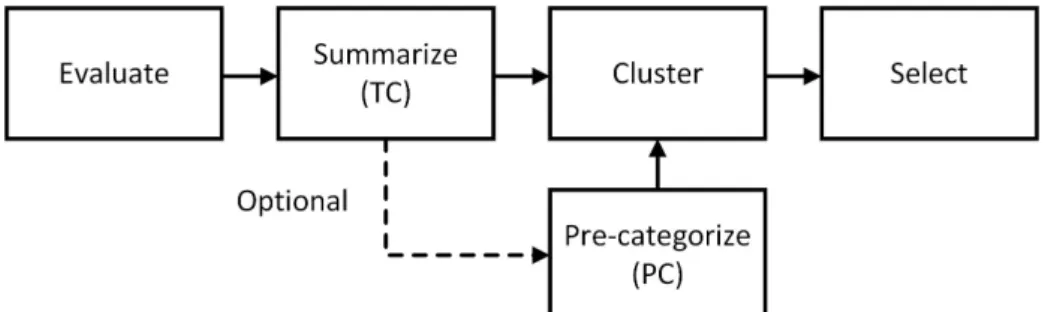
Fig. 1 summarizes the scenario reduction procedure of the customized F-SRC method. Note that pre-categorization of scenarios is an optional step during the cluster phase.
Fig. 1 Scenario reduction procedure of customized FSRC method
4.3 Evaluation of selected scenarios
Instead of comparing similarity in the distributions between selected scenarios and the whole set of scenarios, we evaluate selected sets of scenarios by inves-tigating the performance of the resulting UC schedules against the whole set of scenarios, similar to [44].
For a scenario subsetS0⊆ S, the evaluation procedure is given as: 1. Findf(S0) as in (1) and a corresponding optimal first-stage decision vector
2. Evaluate Q(x0,S) as in (4), and obtain p0gts, αbts0+ and α0−bts, ∀g ∈ G,∀t ∈ T,∀s∈ S
3. Findf(S) and a corresponding optimalx∗. Extractv∗gtfromx∗, and obtain
p∗gts,α∗bts+ andαbts∗−,∀g∈ G,∀t∈ T, s∈ S simultaneously.
4. Compare x0 to x∗, and performance measures U(S0) to U(S), Φ(S|S0) to
Φ(S|S),Ψ+(S|S0) toΨ+(S|S) andΨ−(S|S0) toΨ−(S|S). Definitions ofU(S0),Φ(S|S0),Ψ+(S|S0) andΨ−(S|S0) follow: Commitment cost U(S0) =X t∈T X g∈G cugt(vgt0 ) (22)
Expected generation cost against scenario setS
Φ(S|S0) =X s∈S X t∈T X g∈G ξscpgts(p 0 gts) (23)
Expected shortage and excess against scenario set S
Ψ+(S|S0) =X s∈S X t∈T X b∈B ξsα0bts+ (24) Ψ−(S|S0) =X s∈S X t∈T X b∈B ξsα0−bts (25)
The measures U(S),Φ(S|S), Ψ+(S|S) andΨ−(S|S) are obtained by sub-stitutingv∗gt, p∗gts,α∗bts+ andα∗−bts in (22) - (25).
5 Case studies
The customized FSRC methods are applied to test systems down-sampled from the Independent System Operator of New England (ISO-NE). All 8 load zones in ISO-NE were treated as a single bus in the case studies. To focus on uncertainty associated with net load, outages of transmission and thermal units were not modeled in the case studies, and the associated reserve requirements were also omitted. This section is organized as follows. Section 5.1 briefly describes how net load scenarios were generated. To compare results between FSRC and FFS, we solved single-day SRUC problems on a sample of days from each season as reported in Section 5.2. Section 5.3 further investigates the quality of the scenario sets obtained by FSRC by solving SRUC on a rolling basis for both the selected scenarios and the whole set of original scenarios throughout a week, and comparing their solutions. All case studies of SRUC were solved in their extensive forms by PySP [45, 46] using CPLEX in Windows on a Dell desktop with 8GB memory.
Because of the RAM limitation, subsets of 50 generators are selected from the whole fleet of over 300 generators for the single-day SRUC problems, and 20
generators for SRUC on a rolling horizon basis, to keep computation manage-able. In addition, the 10 highest probability wind energy scenarios are selected from 50 wind energy scenarios to cross with 8 load scenarios which have been generated as described in [47], forming 80 hourly net load scenarios. The net load scenarios were scaled down to match the reduced generation capacity in both case studies. As discussed in Section 4.2, penalties on shortage and excess were initially set to 107$/MWh and 105$/MWh respectively, which are four and two, respectively, orders of magnitude larger than the marginal cost of the most expensive unit, to avoid shortage and excess and emphasize the negative impacts of shortage. In addition, the weightswc, w+ andw− were set to 0.3, 0.4 and 0.3, respectively, to strengthen the emphasis on shortage in clustering.
5.1 Scenario generation
Load scenario generation in this paper started from a historical database of day-ahead hourly weather forecast and corresponding actual hourly load se-quences in 2011 in ISO-NE [48]. Date ranges were identified first to group days according to similarity of the relationship between hourly weather and load, forming “seasons.” This identification of seasons accounted for ad hoc char-acterizations such as diurnal lighting patterns, heating vs. cooling by using air conditioning, and sociological factors including holiday lighting and school being in session or not. In each season, transformations were performed to aggregate data across days of the week and geographic zones. Days in each season were then segmented according to temperature forecast bands. The relationship between hourly loads and weather forecast variables over a day were approximated by a nonparametric regression function and distributions of hourly residuals were approximated as well. Having identified the regres-sion functions and hourly error distributions for each hour in each segment, scenarios were generated as follows, for a given dayD:
1. Identify the season to which day D belongs and the segment to which its weather forecast generated on dayD−1 belongs.
2. Apply the approximated regression function to the weather forecast to get a time-series forecast, and generate the desired number of load scenarios by approximating the distributions of the forecast errors.
3. Invert the transformations to match the day of the week and geographic zone.
For details of this load scenario generation process refer to [47].
Hourly wind scenarios were obtained from a commercial vendor [49] accord-ing to an analogue method [50]. These scenarios were designed to represent a future representing 20% penetration of wind energy in the eastern U.S. in 2024 [51]. Generated load scenarios for 2011 were scaled by the 2.27% increase per year as assumed in [51] to approximate demand levels in 2024. Wind energy was assumed to be nondispatchable, and thereby considered as negative load
in this paper. The net load scenarios representing demands in model (31)-(56) were obtained by subtracting wind energy from load in crossed sets of scenarios.
5.2 Independent daily SRUC
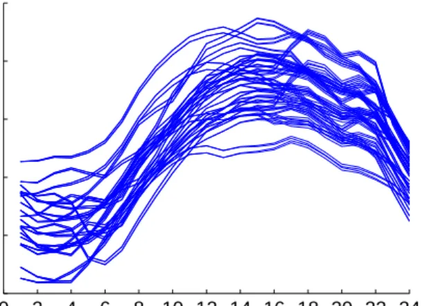
A regular summer week, ranging from 2011-07-10 to 2011-07-16, is selected to test customized FSRC in independent daily SRUC first, and several days are randomly selected from other seasons for testing as well. In independent daily SRUC, the initial status of each generating unit on dayDis independent from its status in the last period on dayD−1. The initial conditions are identified by solving an ED problem for the initial period in which each unit is set on and demand is the expected value for that period over all scenarios. All units for which generation levels are higher than corresponding minimum output,Pg, will be set on, and initial generation levels will be the values derived from the expected value ED problem. To investigate how FSRC performs, subsets of 10, 20, 30, 40, 50 and 60 scenarios are selected from the total 80 net load scenarios by customized FSRC and FFS methods separately. For illustration, the whole set of net load scenarios on day 2011-07-11 are displayed in Fig. 2, and 20 scenarios selected by FFS on the same day are shown in Fig. 3. Assessment of selected scenarios follows the procedure described in Section 4.3.
0 2 4 6 8 10 12 14 16 18 20 22 24 20 40 60 80 100 120 Hour Net load (100 MWh)
Fig. 2 80 net load scenarios on 2011-07-11
Section 5.2.1 provides numerical results of reduced scenarios resulting from solution sensitivity indices created by TC. Section 5.2.2 displays scenario re-duction effects of FSRC when the optional PC step is included.
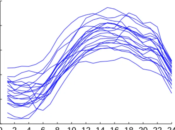
0 2 4 6 8 10 12 14 16 18 20 22 24 20 40 60 80 100 120 Hour Net load (100 MWh)
Fig. 3 20 selected scenarios by FFS on 2011-07-11
5.2.1 Independent daily SRUC: applying TC
The subset of 20 scenarios on 2011-07-11 selected by FSRC with strategy TC is displayed in Fig. 4. Comparisons between Figs. 3 and 4 suggest that scenarios selected by applying TC in FSRC have a wider range than those from FFS , which may indicate that more extreme situations have been retained by FSRC.
0 2 4 6 8 10 12 14 16 18 20 22 24 20 40 60 80 100 120 Hour Net load (100 MWh)
Fig. 4 20 selected scenarios by FSRC: TC on 2011-07-11
For the convenience of describing the comparisons on scenarios which are selected by different methods, S0
F F S denotes the subset of scenarios selected
by FFS, andS0
of the paper. NotationsS0
F SRC:T C andSF SRC0 :T C+P C further distinguish the
two variants of FSRC. Scenario subsets S0
F F S and SF SRC0 :T C are evaluated following the
proce-dure in Section 4.3. Given the whole set of scenarios S, commitment cost,
U(S0
F F S) and U(SF SRC0 :T C), and expected generation costs, Φ(S|SF F S0 ) and
Φ(S|S0
F SRC:T C), are accumulated through the week and displayed in Fig. 5 for
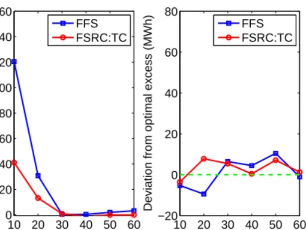
each cardinality, n, of the selected scenario sets. Deviations from the optimal shortage,Ψ+(S|S0 F F S)−Ψ +(S|S) andΨ+(S|S0 F SRC)−Ψ +(S|S), and excess, Ψ−(S|S0
F F S)−Ψ−(S|S) andΨ−(S|SF SRC0 )−Ψ−(S|S), of FFS and FSRC over
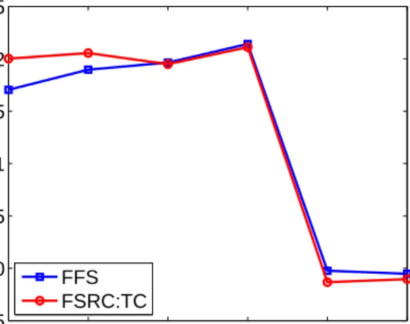
the summer week are displayed in Fig. 6 for each cardinalityn, as well. Fig. 5 shows that, when evaluated over the whole scenario set, commitments from FSRC with the TC strategy and FFS result in similar cost over the summer week for each n. However, the FSRC method causes less expected shortage while resulting in similar levels of excess, as shown in Fig. 6. Fig. 6 also il-lustrates that the expected shortage, Ψ+(S|S0
F SRC), result from FSRC will
better approximateΨ+(S|S) as cardinalitynincreases from 10 to 60.
10 20 30 40 50 60 −0.5 0 0.5 1 1.5 2 2.5
Number of selected scenarios n
Excess from opt. commit. & gen. cost (%)
FFS FSRC:TC
Fig. 5 Deviations from optimal commitment and generation cost of FSRC:TC and FFS through the summer week for different cardinalityn
5.2.2 Independent daily SRUC: applying TC and PC
Pre-categorizing scenarios before clustering is applied to customize FSRC in this section. For comparison, 20 scenarios selected by FSRC with TC and PC on 2011-07-11 are displayed in Fig. 7. Only minor differences can be observed between the sets of selected scenarios shown in Fig. 4 and Fig.7.
Similar to Section 5.2.1, commitment cost,U(SF F S0 ) andU(SF SRC0 :T C+P C), expected generation cost,Φ(S|S0
short-10 20 30 40 50 60 0 20 40 60 80 100 120 140 160 n selected scenarios
Deviation from optimal shortage (MWh)
FFS FSRC:TC 10 20 30 40 50 60 −20 0 20 40 60 80 n selected scenarios
Deviation from optimal excess (MWh)
FFS FSRC:TC
Fig. 6 Deviation from optimal load imbalance of FSRC:TC from FFS through the summer week for different cardinalityn
0 2 4 6 8 10 12 14 16 18 20 22 24 20 40 60 80 100 120 Hour Net load (100 MWh)
Fig. 7 Selected scenarios by FSRC: TC+PC on 2011-07-11
age,Ψ+(S|S0
F F S) andΨ
+(S|S0
F SRC:T C+P C), and expected excess,Ψ
−(S|S0
F F S)
andΨ−(S|S0
F SRC:T C+P C), are accumulated separately through the week, and
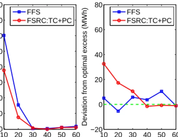
their comparisons are displayed in Figs. 8 and 9. From Fig. 8, applying TC and PC in FSRC will also result in similar commitment and expected generation cost to their counterparts from FFS for differentn. But Fig. 9 shows that FSR-C results in less shortage while yielding not much more excess generation. The absolute value of the savings in excess,|Ψ−(S|S0
F F S)−Ψ−(S|SF SRC0 :T C+P C)|,
dominates the savings in shortage,|Ψ+(S|S0
F F S)−Ψ+(S|SF SRC0 :T C+P C)|, when
n= 30 in Fig. 9. Because there are nearly no differences in shortage, commit-ment and expected generation cost between FFS and FSRC with TC and PC,
the penalty on excess accounts for the higher total expected cost for customized FSRC at this value ofn. 10 20 30 40 50 60 −0.5 0 0.5 1 1.5 2 2.5
Number of selected scenarios n
Excess from opt. commit. & gen. cost (%)
FFS
FSRC:TC+PC
Fig. 8 Deviations from optimal commitment and generation cost of FSRC:TC+PC and FFS through the summer week for different cardinalityn
10 20 30 40 50 60 0 20 40 60 80 100 120 140 160 n selected scenarios
Deviation from optimal shortage (MWh)
FFS FSRC:TC+PC 10 20 30 40 50 60 −20 0 20 40 60 80 n selected scenarios
Deviation from optimal excess (MWh)
FFS
FSRC:TC+PC
Fig. 9 Deviation from optimal load imbalance of FSRC:TC+PC from FFS through the summer week for different cardinalityn
According to these results, the FSRC methods result in less shortage and more economical unit commitments than FFS if a small set of scenarios are selected from the whole set, i.e. fewer than 25% of the whole set of scenarios
are applied to get the UC strategy. The performances of FFS and FSRC are more similar when the cardinality of the selected set is larger (bigger than 40% of the total sceanrios). To assess the performance of selected scenarios especially when n is small, 20 scenarios were selected from the whole set in randomly selected days in spring, fall and winter to run independent daily SRUC. Fig. 10 shows the relative differences in commitment and expected generation cost between FFS and FSRC:
U(S0
F F S) +Φ(S|SF F S0 )− U(SF SRC0 )−Φ(S|SF SRC0 ) U(S0
F F S) +Φ(S|SF F S0 )
×100% (26) for each selected day. The small percentages displayed indicate that scenarios selected by both FSRC variants result in similar costs to those that result from scenarios selected by FFS.
Jan19 Feb05 Mar07 Apr13 Apr26 May03 Sep15 Oct30 Nov09 −5 −4 −3 −2 −1 0 1 2 Date
Diff. in startup and gen. cost (%)
w/o categorization w/ categorization
Fig. 10 Savings in commitment and generation cost of customized FSRC methods from FFS in evaluation
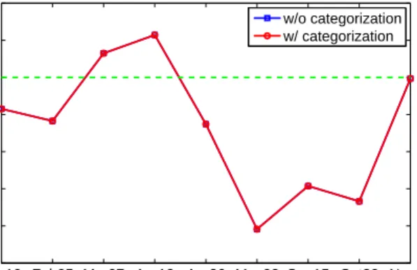
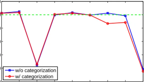
Fig. 11 and Fig. 12 contrast solutions optimized using scenarios selected by FFS and FSRC by showingΨ+(S|S0
F F S)−Ψ
+(S|S0
F SRC) andΨ−(S|SF F S0 )−
Ψ−(S|S0
F SRC), respectively. Fig. 11 illustrates that both of the FSRC variants
usually result in less shortage than FFS in the selected days, while providing similar excess amounts on all but two days (in Fig. 12).
To investigate the sensitivity of FSRC to the penalty parameters used in clustering, different pairs of these parameters were tested. These studies were done for n = 20 because performance of FSRC differs more from FFS when selecting smaller subsets. Fig. 13 displays expected savings in short-age, Ψ+(S|S0
F F S)−Ψ+(S|SF SRC0 ), and excess Ψ−(S|SF F S0 )−Ψ−(S|SF SRC0 )
of FSRC in the summer week which ranges from 2011-07-10 to 2011-07-16. In Fig. 13, UC schedules obtained from both of the FSRC variants result in lower levels of shortage than the schedule obtained from FFS. But applying the TC strategy in FSRC often leads to more excess than applying both TC and PC. In addition, using both TC and PC in FSRC by TC and PC can
Jan19 Feb05 Mar07 Apr13 Apr26 May03 Sep15 Oct30 Nov09 −20 0 20 40 60 80 100 120 Date Savings in shortage (MWh) w/o categorization w/ categorization
Fig. 11 Savings in shortage of FSRC from FFS in evaluations
Jan19 Feb05 Mar07 Apr13 Apr26 May03 Sep15 Oct30 Nov09 −500 −400 −300 −200 −100 0 100 Date
Savings in excess (MWh) w/o categorization
w/ categorization
Fig. 12 Savings in excess of FSRC from FFS in evaluations
sometimes result in both directions of imbalance simultaneously. Overall, the numerical results for the independent daily SRUC testing indicate that the F-SRC methods can result in more economical and reliable schedules compared to FFS.
5.3 Rolling horizon SRUC over a week
Rolling horizon SRUC is performed in the same summer week as tested in Section 5.2. The rolling horizon procedure starts by solving SRUC over 36 hours on daysD andD+ 1, where net load values in a scenario from hour 25 to hour 36 are duplicated from hour 1 to hour 12 in the same scenario. This extension of the daily planning horizon avoids the shut-down of units toward the end of the day that might otherwise occur due to end-of-study effects. The commitment states of units at hour 24 on dayD are adopted as initial states of units on day D+ 1, and the initial generation level (relevant to ramping constraints) of each unit for dayD+ 1 is set to its expected generation over all scenarios at hour 24 of day D. The next two sections describe the
perfor-(4,3)0 (5,3) (6,4) (7,5) (8,6) 20
40 60
Log10 penalty for (shortage, excess) ($,$)
Savings in shortage (MWh) w/o categorization w/ categorization (4,3) (5,3) (6,4) (7,5) (8,6) −40 −20 0 20
Log10 penalty for (shortage, excess) ($,$)
Savings. in excess (MWh)
w/o categorization w/ categorization
Fig. 13 Expected savings in load imbalance of FSRC methods from FFS for 20 selected scenarios through different pairs of penalties
mance of the two variants of FSRC. The UC schedules obtained by optimizing with the reduced sets are evaluated against all scenarios. As in Section 5.2, for scenario subset S0⊆ S,U(S0),Φ(S|S0),Ψ+(S|S0) andΨ−(S|S0) are com-pared to their counterparts if the whole set of scenariosS are used in SRUC. Note that, to perform evaluation of selected scenarios in rolling basis SRUC,
T = {1,· · ·,24} for each day D in formulas (22) - (25). Table 1 shows the commitment cost U(S), expected generation cost Φ(S|S), expected shortage Ψ+(S|S) and excess Ψ−(S|S) evaluated for each day during the week, with the total number of scenarios,|S|= 80, for each day.
Table 1 Expected values of the all-scenarios based SRUC through a week Date U(S) (K$) Φ(S|S) (K$) Ψ+(S|S) (MWh) Ψ−(S|S) (MWh) 2011-07-10 15 712 0 1288 2011-07-11 27 943 96 367 2011-07-12 32 873 13 341 2011-07-13 43 1522 318 37 2011-07-14 26 912 0 0 2011-07-15 32 1309 0 90 2011-07-16 43 1220 3 0 Total 216 7500 431 2124
5.3.1 Rolling horizon SRUC: applying TC
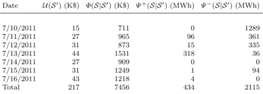
Although the scheduling horizon used in the rolling horizon test includes 36 hours, solution sensitivity indices are computed over 24 hours to select sce-narios for each day. Table 2 summarizes the evaluated daily commitment cost, expected generation cost, and expected load imbalance through the summer week when the cardinality of selected scenarios n= 40. Compared to results from the commitment schedule optimized over all scenarios, entries in Table 2 correspond closely to those in Table 1. Thus, applying TC only in FSRC can yield an acceptable UC strategy even when half of the scenarios are ignored in the optimization.
Table 2 Expected values of UC from TC with respect to all scenarios through a week, n= 40 Date U(S0) (K$) Φ(S|S0) (K$) Ψ+(S|S0) (MWh) Ψ−(S|S0) (MWh) 7/10/2011 15 711 0 1289 7/11/2011 27 965 96 361 7/12/2011 31 873 15 335 7/13/2011 44 1531 318 36 7/14/2011 27 909 0 0 7/15/2011 31 1249 1 94 7/16/2011 43 1218 4 0 Total 217 7456 434 2115
5.3.2 Rolling horizon SRUC: applying TC and PC
Like Table 2, Table 3 shows the evaluation results of applying PC together with TC in FSRC when the cardinality of selected scenariosn= 40. Similar values to those in Table 1 support the use of this variant. Comparisons between Tables 2 and 3 show that both FSRC variants result in similar commitment costs and expected generation costs across the whole set of scenarios, but the combination of TC and PC reduces the expected shortage slightly, and suffers from a litter higher excess.
Another way to compare the results of different selected subsets is to exam-ine the UC schedules directly rather than their evaluation against the whole set of scenarios. Upon concatenating the unit commitment vectors over the days inD, we haveT ={1,2,· · ·,168}. Equation (27) computes the optimal committed capacity given scenario setS0⊆ S.
φt(S0) =
X
g∈G
vgt0 P¯g,∀t∈ T. (27)
The amount of capacity committed in each hour summarizes the schedule. Relative differences ofφt(SF SRC0 :T C) andφt(SF SRC0 :T C+P C) toφt(S) through
Table 3 Expected values of UC from TC+PC with respect to all scenarios through a week, n= 40 Date U(S0) (K$) Φ(S|S0) (K$) Ψ+(S|S0) (MWh) Ψ−(S|S0) (MWh) 7/10/2011 15 712 0 1288 7/11/2011 26 972 96 360 7/12/2011 31 872 13 341 7/13/2011 44 1530 318 36 7/14/2011 27 909 0 0 7/15/2011 33 1243 0 95 7/16/2011 42 1216 4 0 Total 216 7454 432 2120
the week are displayed in Fig. 14. In most hours, both FSRC variants selecting half of the total scenarios provide similar amounts of committed capacity as the optimal schedule.
0 24 48 72 96 120 144 168 −12 −10 −8 −6 −4 −2 0 2 4 6 8 10 12 Hour
Diff. in capacity committed (%)
w/o categorization w/ categorziation
Fig. 14 Relative differences in hourly capacity committed between half-scenarios based rolling horizon SRUC and all-scenarios based rolling horizon SRUC
The quality of scenarios selected by FSRC is further investigated by run-ning rolling horizon SRUC on smaller subsets of selected scenarios. Fig. 15 displays the performances of selected subsets SF SRC0 :T C and SF SRC0 :T C+P C
over days in D according to average hourly relative difference in committed capacity: Z(S0) = 1 |T | X t∈T |φt(S0)−φt(S)| φt(S) (28)
Either variant of FSRC, with or without PC, provides similar capacity commitments to the optimal schedule, when the cardinalitynranges from 10
to 40. Asnincreases, subset-based commitments are closer to optimal. Com-paring the total expected shortage and excess amounts across all scenarios, which are measured byW+(S|S0) andW−(S|S0) separately, provides another view. Fig. 16 displays such comparisons for different cardinalities, and shows that the FSRC variants result in schedules that perform similarly to the rolling schedule optimized using all scenarios in most time, except for that FSRC with PC strategy will lead to an obvious deviation in shortage whenn= 10. Given that about 90% scenarios (70 out of 80 net load scenarios) are ignored for the SRUC, a relative difference around 90% seems to be not much worse for the variant of FSRC with PC strategy. As cardinality n increases from 10, the quality of UC strategy is dramatically improved for the variant of FSRC with PC strategy. Unlike the FSRC variant with PC strategy, only applying TC strategy in FSRC seems to be more reliable than the variant with additional PC strategy. Fig. 16 also illustrates that subsets of scenarios from either vari-ant of FSRC achieve to UC strategies which provide nearly the same expected shortage and excess as those from the whole set of scenarios when cardinality nis above 20. W+(S|S0) = |Ψ+(S|S0)−Ψ+(S|S)| Ψ+(S|S) (29) W−(S|S0) =|Ψ−(S|S0)−Ψ−(S|S)| Ψ−(S|S) (30) 10 20 30 40 0 0.5 1 1.5 2 2.5 3
Number of selected scenarios n
Diff. in capacity committed(%)
w/o categorization w/ categorization
Fig. 15 Z(S0
F SRC:T C) v.s.Z(SF SRC0 :T C+P C) for different cardinalityn
Different pairs of penalty settings on shortage and excess are set to con-duct sensitivity investigations on customized FSRC for rolling horizon SRUC. Fig. 17 shows that Z(S0
dif-10 20 30 40 0 20 40 60 80 100
Number of selected scenarios n
Relative diff. in shortage (%)
(a) w/o categorization w/ categorization 10 20 30 40 0 20 40 60 80 100
Number of selected scenarios n
Relative diff. in excess(%)
(b)
w/o categorization w/ categorization
Fig. 16 Absolute relative differences in expected load imbalance for different car-dinaltiyn: (a)W+(S|S0 F SRC:T C) v.s.W +(S|S0 F SRC:T C+P C), (b)W −(S|S0 F SRC:T C) v.s. W−(S|S0 F SRC:T C+P C)
ferent penalty settings, and subplots in Fig. 18 show thatΨ+(S|S0
F SRC) and
Ψ−(S|S0
F SRC) are not very sensitive to particular values of the penalty factors.
(4,3)0 (5,3) (6,4) (7,5) (8,6) 0.2 0.4 0.6 0.8 1
Log10 penalty on (shortage, excess)($,$)
Diff. in capacity committed (%) w/o categorization
w/ categorization
Fig. 17 Z(S0
F SRC:T C) v.s.Z(S 0
(4,3)0 (5,3) (6,4) (7,5) (8,6) 2 4 6 8 10
Log10 penalty on (shortage, excess)($,$)
Relative diff. in shortage (%)
(a) w/o categorization w/ categorization (4,3)0 (5,3) (6,4) (7,5) (8,6) 2 4 6 8 10
Log10 penalty on (shortage, excess)($,$)
Relative diff. in excess (%)
(b)
w/o categorization w/ categorization
Fig. 18 Relative differences in load imbalances through different penalty set-tings: (a) W+(S|S0 F SRC:T C) v.s. W+(S|S 0 F SRC:T C+P C), (b)W −(S|S0 F SRC:T C) v.s. W−(S|S0 F SRC:T C+P C) 6 Conclusion
In this paper, a scenario reduction method based on solution sensitivity and its customizations for stochastic unit commitment are presented. Numerical investigations on FSRC through single-day and rolling horizon SRUC are per-formed for a sample of days in a case study distilled from data for an indepen-dent system operator in the U.S. Compared to the classical scenario reduction method, FFS, the customized FSRC tracks aspects on which the decision mak-er focuses, and thmak-ereby leads to more reliable unit commitment schedules. In a rolling horizon study, UC schedules obtained with small subsets of scenar-ios selected by the customized FSRC methods are similar to those found by optimizing against the whole set of scenarios. The method uses somewhat ar-tificial penalties on load imbalances but the results are not very sensitive to the particular penalty values used. Tests in this paper were performed on the extensive forms of the two-stage stochastic program, but FSRC could also be used in conjunction with decomposition methods for more efficient solution.
FSRC can be extended easily to a stochastic unit commitment in which variable generation is considered as dispatchable resource. All variable resource generators in that case are considered as elements ofG, and viewed as “always on” units through the schedule horizon by fixing correspondingvgt= 1. The
tech-nique can be applied to select representative scenarios. We expect that in this case, the excess amountsα−bts are likely to be much smaller overall in the UC evaluation because the ability to curtail variable generation will reduce the impact of underestimating wind power on the day ahead.
The proposed scenario reduction method, FSRC, can be further improved by accounting for the nest distance, when selecting a representative scenari-o frscenari-om each scenariscenari-os cluster fscenari-or a twscenari-o-stage scenari-or multi-stage stscenari-ochastic unit commitment model. Similar to the version for the two-stage stochastic unit commitment, a feasible UC strategy will be applied to evaluate scenarios, and decisions at each stage will be elements to create solution sensitivity indices in a multi-stage stochastic unit commitment. To avoid overly complicated so-lution sensitivity indices as the number of stages increase, further research is required to identify efficient ways to summarize multistage solution sensitivity.
References
1. S. Takriti, J. Birge, and E. Long. A stochastic model for the unit commitment problem.
IEEE Transactions on Power Systems, 11(3):1497–1508, 1996.
2. P. Carpentier, G. Gohen, J-C Culioli, and A. Renaud. Stochastic optimization of unit commitment: a new decomposition framework.IEEE Transactions on Power Systems, 11(2):1067–1073, 1996.
3. J. Dupaˇcov´a, N. Gr¨owe-Kuska, and W. R¨omisch. Scenario reduction in stochastic programming: an approach using probability metrics. Mathematical programming, 95(3):493–511, 2003.
4. H. Heitsch and W. R¨omisch. Scenario reduction algorithms in stochastic programming.
Computational optimization and applications, 24(2):187–206, 2003.
5. A. Botterud, Z. Zhou, J. Wang, J. Valenzuela, J. Sumaili, R.J. Bessa, H. Keko, and V. Miranda. Unit commitment and operating reserves with probabilistic wind power forecasts. InPowerTech, 2011 IEEE Trondheim, pages 1–7. IEEE, 2011.
6. A. Papavasiliou and S. Oren. Multiarea stochastic unit commitment for high wind penetration in a transmission constrained network.Operations Research, 2013. 7. A. Papavasiliou, S. Oren, and R. O’Neill. Reserve requirements for wind power
inte-gration: A scenario-based stochastic programming framework. IEEE Transactions on Power Systems, 26(4):2197–2206, 2011.
8. F. Bouffard, F. Galiana, and A. Conejo. Market-clearing with stochastic security-part i: formulation.IEEE Transactions on Power Systems, 20(4):1818–1826, 2005. 9. F. Bouffard and F. Galiana. Stochastic security for operations planning with significant
wind power generation.IEEE Transactions on Power Systems, 23(2):306–316, 2008. 10. J. Morales, A. J. Conejo, K. Liu, and J. Zhong. Pricing electricity in pools with wind
producers.IEEE Transactions on Power Systems, 27(3):1366–1376, 2012.
11. A. Tuohy, P. Meibom, E. Denny, and M. O’Malley. Unit commitment for systems with significant wind penetration. IEEE Transactions on Power Systems, 24(2):592–601, 2009.
12. P. Ruiz, C. Philbrick, E. Zak, K. Cheung, and P. Sauer. Uncertainty management in the unit commitment problem. IEEE Transactions on Power Systems, 24(2):642–651, 2009.
13. E. Constantinescu, V. Zavala, M. Rocklin, S. Lee, and M. Anitescu. A computational framework for uncertainty quantification and stochastic optimization in unit commit-ment with wind power generation. IEEE Transactions on Power Systems, 26(1):431– 441, 2011.
14. W. R¨omisch and S. Vigerske. Recent progress in two-stage mixed-integer stochastic programming with applications to power production planning. InHandbook of Power Systems I, pages 177–208. Springer, 2010.
15. Q. Zheng, J. Wang, P. Pardalos, and Y. Guan. A decomposition approach to the two-stage stochastic unit commitment problem.Annals of Operations Research, pages 1–24, 2012.
16. C. Carøe and R. Schultz. A two-stage stochastic program for unit commitment under uncertainty in a hydro-thermal power system. DFG-Schwerpunktprogramm Echtzeit-Optimierung großer Systeme,Preprint, 98-13, 1998.
17. M. Nowak and W. R¨omisch. Stochastic lagrangian relaxation applied to power schedul-ing in a hydro-thermal system under uncertainty.Annals of Operations Research, 100(1-4):251–272, 2000.
18. J-P. Watson and D. Woodruff. Progressive hedging innovations for a class of stochas-tic mixed-integer resource allocation problems. Computational Management Science, 8(4):355–370, 2011.
19. J. Dupaˇcov´a, G. Consigli, and S.W. Wallace. Scenarios for multistage stochastic pro-grams.Annals of operations research, 100(1):25–53, 2000.
20. A. Philpott, M. Craddock, and H. Waterer. Hydro-electric unit commitment subject to uncertain demand.European Journal of Operational Research, 125(2):410–424, 2000. 21. J. M. Latorre, S. Cerisola, and A. Ramos. Clustering algorithms for scenario tree
generation: Application to natural hydro inflows. European Journal of Operational Research, 181(3):1339–1353, 2007.
22. C. K¨uchler and S. Vigerske. Decomposition of multistage stochastic programs with recombining scenario trees.Stochastic Programming E-Print Series (SPEPS). 23. A. J. Kleywegt, A. Shapiro, and T. Homem-de Mello. The sample average approximation
method for stochastic discrete optimization.SIAM Journal on Optimization, 12(2):479– 502, 2002.
24. M. Dempster and R. Thompson. Evpi-based importance sampling solution procedures-for multistage stochastic linear programmes on parallel mimd architectures.Annals of Operations Research, 90:161–184, 1999.
25. A. Beltratti, A. Consiglio, and S. A. Zenios. Scenario modeling for the management ofinternational bond portfolios.Annals of Operations Research, 85:227–247, 1999. 26. M. Bertocchi, V. Moriggia, and J. Dupaˇcov´a. Sensitivity of bond portfolio’s
behav-ior with respect to random movements in yield curve: A simulation study. Annals of Operations Research, 99(1-4):267–286, 2000.
27. D. Carino, D. Myers, and W. Ziemba. Concepts, technical issues, and uses of the russell-yasuda kasai financial planning model.Operations Research, 46(4):450–462, 1998. 28. H. Heitsch and W. R¨omisch. A note on scenario reduction for two-stage stochastic
programs.Operations Research Letters, 35(6):731–738, 2007.
29. R. Henrion, C. K¨uchler, and W. R¨omisch. Scenario reduction in stochastic programming with respect to discrepancy distances. Computational Optimization and Applications, 43(1):67–93, 2009.
30. R. Henrion, C. K¨uchler, and W. R¨omisch. Discrepancy distances and scenario reduction in twostage stochastic mixed-integer programming.Journal of Industrial and Manage-ment Optimization, 4(2):363–384, 2008.
31. H. Heitsch, W. R¨omisch, and C. Strugarek. Stability of multistage stochastic programs.
SIAM Journal on Optimization, 17(2):511–525, 2006.
32. H. Heitsch and W. R¨omisch. Scenario tree reduction for multistage stochastic programs.
Computational Management Science, 6(2):117–133, 2009.
33. H. Heitsch and W. R¨omisch. Scenario tree modeling for multistage stochastic programs.
Mathematical Programming, 118(2):371–406, 2009.
34. H. Heitsch and W. R¨omisch. Stability and scenario trees for multistage stochastic programs.Stochastic Programming, pages 139–164, 2011.
35. L. Wu, M. Shahidehpour, and T. Li. Stochastic security-constrained unit commitment.
IEEE Transactions on Power Systems, 22(2):800–811, 2007.
36. J. Wang, M. Shahidehpour, and Z. Li. Security-constrained unit commitment with volatile wind power generation. IEEE Transactions on Power Systems, 23(3):1319– 1327, 2008.
37. J.M. Morales, S. Pineda, A.J. Conejo, and M. Carrion. Scenario reduction for futures market trading in electricity markets.IEEE Transactions on Power Systems, 24(2):878– 888, 2009.
38. N. Growe-Kuska, H. Heitsch, and W. Romisch. Scenario reduction and scenario tree construction for power management problems. InIEEE Bologna Power Tech Conference Proceedings, 2003.
39. S-E Fleten and S. W. Wallace. Delta-hedging a hydropower plant using stochastic programming. InOptimization in the energy industry, pages 507–524. Springer, 2009. 40. Georg Ch. Pflug and Alois Pichler. A distance for multistage stochastic optimization
models.SIAM Journal on Optimization, 22(1):1–23, 2012.
41. Anna V Timonina. Multi-stage stochastic optimization: the distance between stochastic scenario processes.Computational Management Science, pages 1–25, 2013.
42. Y. Feng and S. M. Ryan. Scenario construction and reduction applied to stochastic power generation expansion planning. Computers & Operations Research, 40(1):9–23, 2013.
43. M. Carri´on and J.M. Arroyo. A computationally efficient mixed-integer linear formula-tion for the thermal unit commitment problem.IEEE Transactions on Power Systems, 21(3):1371–1378, 2006.
44. M. Kaut and S.W. Wallace. Evaluation of scenario-generation methods for stochastic programming.Pacific Journal of Optimization, 3(2):257–271, 2007.
45. J-P Watson, D. Woodruff, and W. Hart. Pysp: modeling and solving stochastic programs in python.Mathematical Programming Computation, 4(2):109–149, 2012.
46. Sandia National Laboratories. Pysp. https://software.sandia.gov/trac/coopr/wiki/PySP. 47. Y. Feng, I. Rios, S. Ryan, K. Sp¨urkel, Watson J., R. Wets, and D Woodruff. Scalable
stochastic unit commitment - part 1: scenario generation.Under review.
48. ISO-NE. Hourly zonal information. http://www.iso-ne.com/markets/hstdata/znl info/hourly/index.html.
49. 3TIER Inc. Private communication. http://www.3tier.com/en/.
50. W. Mahoney, K. Parks, G. Wiener, Y. Liu, W. Myers, J. Sun, L. Delle Monache, T. Hop-son, D. JohnHop-son, and S. E. Haupt. A wind power forecasting system to optimize grid integration.IEEE Transactions on Sustainable Energy, 3(4):670 – 682, 2011.
51. D. Corbus, J. King, T. Mousseau, R. Zavadil, B. Heath, L. Hecker, J. Lawhorn, D. Os-born, J. Smit, R. Hunt, et al. Eastern wind integration and transmission study.NREL (http://www. nrel. gov/docs/fy09osti/46505. pdf ), CP-550-46505, 2010.