EVALUATION OF STOCHASTIC
OPTIMISATION ALGORITHMS FOR
INDUCTION MACHINE WINDING FAULT
IDENTIFICATION
Mohamoud Omran A. Alamyal
B.Sc., M.Sc.
A thesis submitted for the degree of
Doctor of Philosophy
June, 2012
School of Electrical and Electronic Engineering
Newcastle University
United Kingdom
II
ABSTRACT
This thesis is concerned with parameters identification and winding fault detection in induction motors using three different stochastic optimisation algorithms, namely genetic algorithm (GA), tabu search (TS) and simulated annealing (SA).
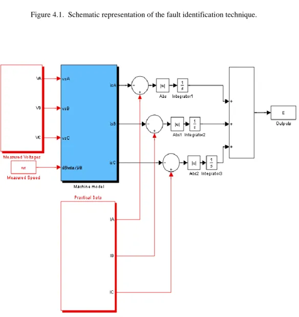
Although induction motors are highly reliable, require low maintenance and have relatively high efficiency, they are subject to many electrical and mechanical types of faults. Undetected faults can lead to serious machine failures. Fault identification is, therefore, essential in order to detect and diagnose potential failures in electrical motors. Conventional methods of fault detection usually involve embedding sensors in the machines, but these are very expensive. The condition monitoring technique proposed in this thesis flags the presence of a winding fault and provides information about its nature and location by using an optimisation stochastic algorithm in conjunction with measured time domain voltage, stator current data and rotor speed data. This technique requires a mathematical ABCabc model of the three-phase induction motor.
The performance of the three stochastic search methods is evaluated in this thesis for their use to identify open-circuit faults in the stator and rotor windings of a three-phase induction motor. The proposed fault detection technique is validated through the use of experimental data collected under steady-state operating conditions. Time domain terminal voltages and the rotor speed are used as input data for the induction motor model while the outputs are the calculated stator currents. These calculated currents are compared to the measured currents to produce a set of current errors that are integrated and summed to give an overall error function. Fault
III
identification is achieved by adjusting the model parameters off-line using the stochastic search method to minimise this error function. The estimate values for the winding parameters give the best possible match between the performance of the faulty experimental machine and its mathematical ABCabc model. These estimates of the values of the motor winding parameters are used in the detection of the development of faults by identifying both the location and the nature of the winding fault. The effectiveness of the three stochastic methods to identify stator and rotor winding faults are compared in terms of the required computation resources and their success rates in converging to a solution.
IV
Acknowledgements
First of all, my deepest gratitude is due to God, the most graceful and the most merciful for his blessings.
I would like to express my sincere gratitude to my supervisor Dr. Bashar Zahawi for his guidance, advices and support throughout the duration of this work.
Thanks also go to my second supervisor Dr. Damian Giaouris for his help and support. Moreover, I would like to thank my friends and colleagues at Newcastle University for the wonderful discussions and friendly working atmosphere during my stay here.
I deeply appreciate the scholarship awarded to me to do this research degree by the Ministry of Higher Education of Libyan Government.
Lastly, I would like to thank my parents, my wife and my lovely children for their support, care and love.
V
TABLE OF CONTENTS
CHAPTER 1: INTRODUCTION ... 1
1.1 Overview of thesis ... 2
1.2 Contributions ... 3
CHAPTER 2: LITERATURE REVIEW ... 5
2.1 Introduction ... 5
2.2 Induction Machine Faults ... 7
2.2.1 Electrical faults... 8 2.2.1.1 Stator faults ... 8 2.2.1.2 Rotor Faults ... 9 2.2.2 Mechanical Faults ... 9 2.2.2.1 Bearing Faults ... 9 2.2.2.2 Eccentricity fault ... 10 2.2.3 Other Faults ... 12
2.3 Fault detection Methods ... 12
2.3.1 Motor current signature analysis ... 12
2.3.2 Artificial Intelligence diagnoses ... 13
2.3.2.1 Neural Networks ... 13
VI
2.3.3 Park’s Vector Approach ... 14
2.3.4 Stochastic optimisation search methods ... 14
2.3.4.1 Tabu search ... 15
2.3.4.2 Genetic Algorithm ... 16
2.3.4.3 Simulated Annealing ... 16
CHAPTER 3: STOCHASTIC OPTIMISATION ALGORITHMS ... 18
3.1 Introduction ... 18
3.2 Genetic Algorithm ... 20
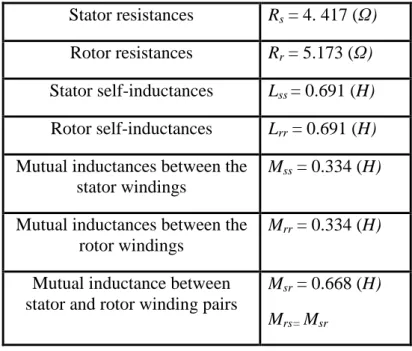
3.2.1 Introduction ... 20
3.2.2 Basic concept of genetic algorithm ... 21
3.2.2.1 Initialisation ... 23
3.2.2.2 Objective function and fitness functions ... 23
3.2.2.3 Selection ... 23
3.2.2.4 Crossover ... 25
3.2.2.5 Mutation ... 26
3.2.3 Reinsertion ... 27
3.2.4 Application of GA to simple example ... 27
3.3 Tabu Search ... 29
3.3.1 Introduction ... 29
3.3.2 Tabu Search Procedure ... 29
3.3.3 The Tabu List ... 31
VII
3.3.5 Application of TS to a simple example ... 32
3.4 Simulated annealing ... 33
3.4.1 Introduction ... 33
3.4.2 Basic concepts of simulated annealing ... 34
3.4.3 SA procedure ... 36
3.4.4 Cooling schedule ... 38
3.4.5 Application of SA to simple examples... 39
3.5 Summary ... 40
CHAPTER 4: CONDITION MONITORING SCHEME, EXPERIMENTAL SET-UP AND TEST DATA ... 41
4.1 Introduction ... 41
4.2 Condition monitoring scheme ... 41
4.3 Test rig ... 44
4.4 Experimental results ... 49
4.4.1 Healthy Machine Tests ... 49
4.4.2 Stator open-circuit winding fault ... 51
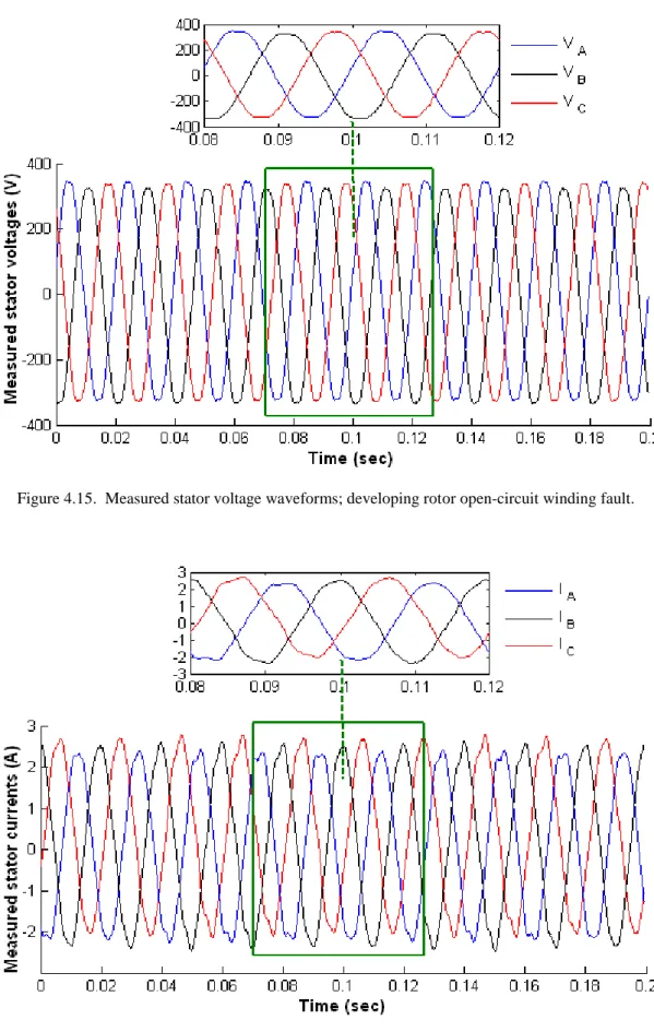
4.4.3 Rotor open-circuit winding fault ... 53
4.5 Summary ... 55
CHAPTER 5: USE OF GENETIC ALGORITHM FOR INDUCTION MOTOR FAULT DETECTION AND PARAMETERS IDENTIFICATION ... 56
5.1 Introduction ... 56
5.2 Induction machine parameter identification using GA ... 57
VIII
5.3.1 Supply-fed induction motor ... 61
5.3.1.1 Stator open-circuit winding fault ... 61
5.3.1.2 Rotor open-circuit winding fault ... 65
5.3.2 Inverter-fed induction motor ... 69
5.3.2.1 Stator open-circuit winding fault ... 70
5.3.2.2 Rotor open-circuit winding fault ... 73
5.4 Summary ... 75
CHAPTER 6: USE OF TABU SEARCH FOR INDUCTION MOTOR FAULT DETECTION AND PARAMETERS IDENTIFICATION ... 77
6.1 Introduction ... 77
6.2 Induction machine parameter identification using TS ... 78
6.3 Winding Fault detection ... 81
6.3.1 Supply-fed induction motor ... 81
6.3.1.1 Stator winding open-circuit fault ... 81
6.3.1.2 Rotor winding open-circuit fault ... 84
6.3.2 Inverter-fed induction motor ... 87
6.3.2.1 Stator winding open-circuit fault ... 87
6.3.2.2 Rotor winding open-circuit fault ... 90
6.4 Summary ... 93
CHAPTER 7: USE OF SIMULATED ANNEALING FOR INDUCTION MOTOR FAULT DETECTION AND PARAMETERS IDENTIFICATION. .. 94
7.1 Introduction ... 94
IX
7.3 Winding fault detection ... 95
7.3.1 Supply-fed induction motor ... 95
7.3.1.1 Stator winding open circuit fault ... 95
7.3.1.2 Rotor winding open-circuit fault ... 98
7.3.2 Inverter-fed induction motor ... 101
7.3.2.1 Stator winding open-circuit fault ... 101
7.3.2.2 Rotor winding open-circuit fault ... 104
7.4 Summary ... 106
CHAPTER 8: THESIS CONCLUSION AND FUTURE WORK ... 107
8.1 Conclusion... 107
8.2 Future work ... 109
REFERENCES… ... 110
X
LIST OF FIGURES
Figure 2.1. Types of induction machine faults. ... 8
Figure 2.2. Possible failure modes in induction machine stator windings. ... 9
Figure 2.3. A schematic view of rolling element bearings ... 10
Figure 2. 4. Cross section of a healthy induction motor. ... 11
Figure 2.5. Static eccentricity... 11
Figure 2.6. Dynamic eccentricity. ... 11
Figure 3.1. Classification of stochastic optimisation algorithms. ... 19
Figure 3.2. The basic cycle of Evolutionary Algorithms. ... 21
Figure 3.3. GA flowchart. ... 22
Figure 3.4. An example of roulette wheel selection... 24
Figure 3.5. The GA crossover operation. ... 26
Figure 3.6. Illustration of mutation in Genetic Algorithms. ... 27
Figure 3.7. Function with a local minimum. ... 28
Figure 3.8. Value of potential solution and objective function obtained by GA. ... 28
Figure 3.9. The flowchart for tabu search algorithm. ... 31
Figure 3.10. Value of potential solution and objective function obtained by TS. .... 33
Figure 3.11. The flowchart of the Simulated Annealing algorithm. ... 36
XI
Figure 4.1. Schematic representation of the fault identification technique. ... 43
Figure 4.2. Simulink model showing machine mathematical model combined with practical data. ... 43
Figure 4.3. Schematic diagram of the experimental set-up [85]. ... 45
Figure 4.4. The experimental test rig. ... 46
Figure 4.5. Induction machine connection diagram [85]. ... 46
Figure 4.6. View of test machine front plate. ... 47
Figure 4.7. Measured (IA, IB, IC) and calculated (IsA, IsB, IsC) stator current waveforms using the estimated parameters obtained from IEEE standard tests. ... 48
Figure 4.8. Healthy conditions. ... 49
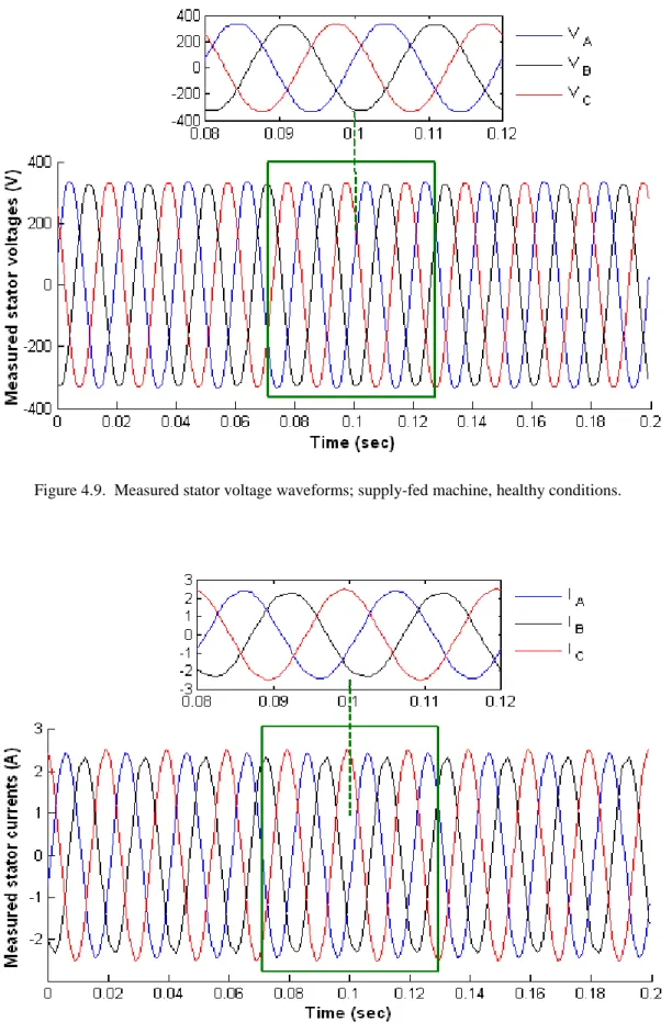
Figure 4.9. Measured stator voltage waveforms; supply-fed machine, healthy conditions. ... 50
Figure 4.10. Measured stator current waveforms; supply-fed machine, healthy conditions. ... 50
Figure 4.11. Developing stator winding open-circuit fault; test circuit. ... 51
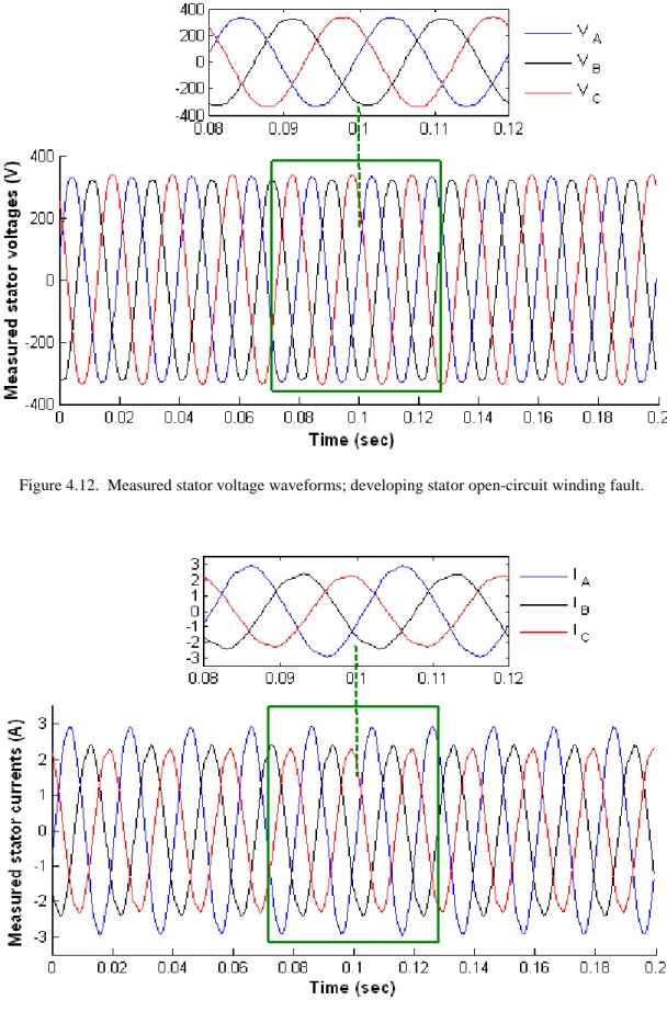
Figure 4.12. Measured stator voltage waveforms; developing stator open-circuit winding fault. ... 52
Figure 4.13. Measured stator current waveforms; developing stator open-circuit winding fault. ... 52
XII
Figure 4.15. Measured stator voltage waveforms; developing rotor open-circuit winding fault. ... 54 Figure 4.16. Measured stator current waveforms; developing rotor open-circuit winding. ... 54
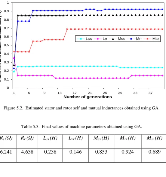
Figure 5.1. Estimated stator and rotor resistances obtained using GA. ... 58 Figure 5.2. Estimated stator and rotor self and mutual inductances obtained using GA. ... 59 Figure 5.3. Estimated calculation error for parameter estimation obtained using GA. ... 60 Figure 5.4. Measured (IA, IB, IC) and calculated (IsA, IsB, IsC) stator current
waveforms using the estimated parameters obtained from GA. ... 60
Figure 5.5. Developing stator winding open-circuit fault; test circuit. ... 62 Figure 5.6. Estimated stator resistances obtained using GA for operation of induction motor with stator open-circuit fault. ... 63 Figure 5.7. Estimated rotor resistances obtained using GA for operation of induction motor with stator open-circuit fault. ... 63
Figure 5.8. Estimated calculation error obtained using GA for operation of induction motor with stator open-circuit fault. ... 64 Figure 5.9. Measured (IA, IB, IC) and calculated (IsA, IsB, IsC) stator current
XIII
induction motor with stator open-circuit fault. ... 65 Figure 5.10. Developing rotor winding open-circuit fault; test circuit. ... 65 Figure 5.11. Estimated rotor resistances obtained using GA for operation of induction motor with rotor open-circuit fault. ... 66 Figure 5.12. Estimated stator resistances obtained using GA for operation of induction motor with rotor open-circuit fault. ... 67 Figure 5.13. Estimated calculation error obtained using GA for operation of induction motor with rotor open-circuit fault. ... 68 Figure 5.14. Measured (IA, IB, IC) and calculated (IsA, IsB, IsC) stator current
waveforms using the estimated resistances obtained from GA for operation of induction motor with rotor open-circuit fault. ... 68 Figure 5.15 Simulink model showing machine mathematical model combined with machine mathematical model supplied by PWM (practical data) ... 69
Figure 5.16. Estimated stator resistances obtained using GA for operation of inverter-fed induction motor with stator open-circuit fault at 40 Hz stator frequency. ... 70 Figure 5.17. Estimated rotor resistances obtained using GA for operation of inverter-fed induction motor with stator open-circuit fault at 40 Hz stator frequency. ... 71
Figure 5.18. Estimated calculation error obtained using GA for operation of inverter-fed induction motor with stator open-circuit fault at 40 Hz stator frequency. ... 71
XIV
Figure 5.19. Measured (IA, IB, IC) and calculated (IsA, IsB, IsC) stator current
waveforms using the estimated resistances obtained from GA for operation of inverter-fed induction motor with stator open-circuit fault at 40 Hz stator frequency. ... 72 Figure 5.20. Estimated rotor resistances obtained using GA for operation of inverter-fed induction motor with rotor open-circuit fault at 40 Hz stator frequency. ... 73 Figure 5.21. Estimated stator resistances obtained using GA for operation of inverter-fed induction motor with rotor open-circuit fault at 40 Hz stator frequency. ... 74 Figure 5.22. Estimated calculation error obtained using GA for operation of inverter-fed induction motor with rotor open-circuit fault at 40 Hz stator frequency. ... 74 Figure 5.23. Measured (IA, IB, IC) and calculated (IsA, IsB, IsC) stator current
waveforms using the estimated resistances obtained from GA for operation of inverter-fed induction motor with rotor open-circuit fault at 40 Hz stator frequency. ... 75
Figure 6.1. Estimated stator and rotor resistances obtained using TS algorithm. ... 79 Figure 6.2. Estimated stator and rotor self and mutual inductances obtained using TS. ... 79 Figure 6.3. Estimated calculation error for parameter estimation obtained using TS. ... 80
XV
Figure 6.4. Measured (IA, IB, IC) and calculated (IsA, IsB, IsC) stator current
waveforms using the estimated parameters obtained from TS. ... 80 Figure 6.5. Estimated stator resistances obtained using TS for operation of induction motor with stator open-circuit fault. ... 82 Figure 6.6. Estimated rotor resistances obtained using TS for operation of induction motor with stator open-circuit fault. ... 82 Figure 6.7. Estimated calculation error obtained using TS for operation of induction motor with stator open-circuit fault. ... 83 Figure 6.8. Measured (IA, IB, IC) and calculated (IsA, IsB, IsC ) stator current
waveforms using the estimated resistances obtained from TS for operation of induction motor with stator open-circuit fault. ... 84 Figure 6.9. Estimated rotor resistances obtained using TS for operation of induction motor with rotor open-circuit fault. ... 85
Figure 6.10. Estimated stator resistances obtained using TS for operation of induction motor with rotor open-circuit fault. ... 85
Figure 6.11. Estimated calculation error obtained using TS for operation of induction motor with rotor open-circuit fault. ... 86 Figure 6.12. Measured (IA, IB, IC) and calculated (IsA, IsB, IsC ) stator current
waveforms using the estimated resistances obtained from TS for operation of induction motor with rotor open-circuit fault. ... 87 Figure 6.13. Estimated stator resistances obtained using TS for operation of
inverter-XVI
fed induction motor with stator open-circuit fault at 40 Hz stator frequency. ... 88 Figure 6.14. Estimated rotor resistances obtained using TS for operation of inverter-fed induction motor with stator open-circuit fault at 40 Hz stator frequency. ... 88
Figure 6.15. Estimated calculation error obtained using TS for operation of inverter-fed induction motor with stator open-circuit fault at 40 Hz stator frequency. ... 89
Figure 6.16. Measured (IA, IB, IC) and calculated (IsA, IsB, IsC ) stator current
waveforms using the estimated resistances obtained from TS for operation of inverter-fed induction motor with stator open-circuit fault at 40 Hz stator frequency. ... 90 Figure 6.17. Estimated rotor resistances obtained using TS for operation of inverter-fed induction motor with rotor open-circuit fault at 40 Hz stator frequency. ... 91 Figure 6.18. Estimated stator resistances obtained using TS for operation of inverter-fed induction motor with rotor open-circuit fault at 40 Hz stator frequency. ... 91
Figure 6.19. Estimated calculation error obtained using TS for operation of inverter-fed induction motor with rotor open-circuit fault at 40 Hz stator frequency. ... 92
Figure 6.20. Measured (IA, IB, IC) and calculated (IsA, IsB, IsC ) stator current
waveforms using the estimated resistances obtained from TS for operation of inverter-fed induction motor with rotor open-circuit fault at 40 Hz stator frequency. ... 93
Figure 7.1. Estimated stator resistances obtained using SA for operation of induction motor with stator open-circuit fault. ... 96
XVII
Figure 7.2. Estimated rotor resistances obtained using SA for operation of induction motor with stator open-circuit fault. ... 96 Figure 7.3. Estimated calculation error obtained using SA for operation of induction motor with stator open-circuit fault. ... 97 Figure 7.4. Measured (IA, IB, IC) and calculated (IsA, IsB, IsC) stator current
waveforms using the estimated resistances obtained from SA for operation of induction motor with stator open-circuit fault ... 98 Figure 7.5. Estimated rotor resistances obtained using SA for operation of induction motor with rotor open-circuit fault. ... 99 Figure 7.6. Estimated stator resistances obtained using SA for operation of induction motor with rotor open-circuit fault. ... 99 Figure 7.7. Estimated calculation error obtained using SA for operation of induction motor with rotor open-circuit fault. ... 100
Figure 7.8. Measured (IA, IB, IC) and calculated (IsA, IsB, IsC) stator current
waveforms using the estimated resistances obtained from SA for operation of induction motor under a rotor open-circuit fault. ... 101 Figure 7.9. Estimated stator resistances obtained using SA for operation of inverter-fed induction motor with stator open-circuit fault at 40 Hz stator frequency. ... 102 Figure 7.10. Estimated rotor resistances obtained using SA for operation of inverter-fed induction motor with stator open-circuit fault at 40 Hz stator frequency. ... 102 Figure 7.11. Estimated calculation error obtained using SA for operation of
inverter-XVIII
fed induction motor with stator open-circuit fault at 40 Hz stator frequency. ... 103 Figure 7.12. Measured (IA, IB, IC) and calculated (IsA, IsB, IsC) stator current
waveforms using the estimated resistances obtained from SA for operation of inverter-fed induction motor with stator open-circuit fault at 40 Hz stator frequency. ... 104 Figure 7.13. Estimated rotor resistances obtained using SA for operation of inverter-fed induction motor with rotor open-circuit fault at 40 Hz stator frequency. ... 105 Figure 7.14. Estimated stator resistances obtained using SA for operation of inverter-fed induction motor with rotor open-circuit fault at 40 Hz stator frequency. ... 105
Figure 7.15. Estimated calculation error obtained using SA for operation of inverter-fed induction motor with rotor open-circuit fault at 40 Hz stator frequency. ... 106
XIX
LIST OF tables
Table 4.1. Induction motor model parameters. ... 48
Table 5.1. GA parameter values. ... 57
Table 5.2. Search space for machine parameters. ... 58
Table 5.3. Final values of machine parameters obtained using GA. ... 59
Table 5.4. Final values of winding resistances obtained using GA with stator open-circuit fault. ... 64
Table 5.5. Final values of winding resistances obtained using GA with rotor open-circuit fault. ... 67
Table 5.6. Final values of winding resistances obtained using GA with stator open-circuit fault at 40 Hz stator frequency. ... 72
Table 5.7. Final values of winding resistances obtained using GA with rotor open-circuit fault at 40 Hz stator frequency. ... 75
Table 6.1. Final values of machine parameters obtained using TS algorithm. ... 78
Table 6.2. Final values of winding resistances obtained using TS with stator open-circuit fault. ... 83
Table 6.3. Final values of winding resistances obtained using TS with rotor open-circuit fault. ... 86
XX
Table 6.4. Final values of winding resistances obtained using TS with stator open-circuit fault at 40 Hz stator frequency. ... 89 Table 6.5. Final values of winding resistances obtained using TS with rotor open-circuit fault at 40 Hz stator frequency. ... 92
Table 7.1. Final values of winding resistances obtained using SA with stator open-circuit fault. ... 97
Table 7.2. Final values of winding resistances obtained using SA with rotor open-circuit fault. ... 100 Table 7.3. Final values of winding resistances obtained using SA with a stator open-circuit fault at 40 Hz stator frequency. ... 103 Table 7.4. Final values of winding resistances obtained using SA with rotor open-circuit fault at 40 Hz stator frequency. ... 106
XXI
List of Principal symbols
and abbreviations
Below is a list of symbols and abbreviation that are used throughout this thesis. When possible the meaning of each symbol is given in the text when the symbol is first used.
RsA, RsB, RsC Stator Resistances
Rra, Rrb, Rrc Rotor Resistances
VsA, VsB, VsC Stator voltages
IsA, IsB, IsC Stator Currents
Ira, Irb, Irc Rotor Currents
LsA, LsB, LsC Stator Self Inductances
Mss Mutual Inductance between pairs of stator windings
Lra, Lrb, Lrc Rotor Self Inductances
Mrr Mutual inductance between pairs of rotor windings
Msr = Mrs Mutual inductance between stator/rotor winding
Lm Stator to Rotor Mutual Inductance
w Angular rotor speed
r
Rotor position angle
DC Direct Current GA Genetic Algorithm
XXII SA Simulated Annealing TS Tabu Search
ACO Ant Colony Optimisation PSO Particle Swarm Optimisation BFO Bacterial Forging Optimisation Ls Tabu list
Lst Length of the string.
T Temperature Ts Initial temperature
PA Acceptance probability
Ps Swap probability
AI Artificial intelligence ANNs Artificial neural networks FLS Fuzzy logic systems
MCSA Motor current signature analysis SOA Stochastic optimisation algorithms
CHAPTER-1 Introduction
1
CHAPTER 1
INTRODUCTION
The three-phase induction motor is used in a wide variety of applications because of its simple, rugged construction, easy maintenance, low cost and good operating characteristics. It is an electromechanical energy device in which the energy is converted from electrical to mechanical form. Although induction motors are highly reliable and have relatively high efficiency, they are subject to many types of faults. The ability to test the integrity of the motor through this process results in lower maintenance costs and an overall lowered risk of malfunction. Conventional methods of condition monitoring are based on a variety of technologies including vibration analysis and current signature analysis.
Condition monitoring of induction motor is usually applied to detect various types of electrical and mechanical faults. It is important to be able to detect faults while they are still developing. This called incipient failure detection. A fault that is not identified in the initial stage may become catastrophic and the induction motor may suffer severe damage. Thus, undetected motor faults may result in motor failure and complete shutdown of the machine. Such shutdowns are very costly in terms of lost production time, wasted raw materials and maintenance costs. Condition monitoring is necessary for identifying machine defects and their location. Knowledge of the motor condition allows the operator to review the physical state of the motor so as to prevent machine damage by stopping the process and carrying out the required maintenance at an appropriate time. The application of condition monitoring in plants results in savings in maintenance costs, and improved safety. Therefore, many condition monitoring techniques have been proposed and applied to the fault
CHAPTER-1 Introduction
2 detection of three-phase induction motors [1-15].
A new method for detecting induction motor faults based on global random optimisation methods has recently been developed [16]. This technique has the potential to identify a wide variety of faults without the need for knowledge of various fault signatures. However, this method requires the measurement of the rotor position angle θ, limiting the potential use of this approach because of the implied extra cost and complexity. In this work, this technique is developed and is also applied for inverter-fed induction motor using different stochastic methods; no rotor position is required for the proposed technique. The proposed technique uses only terminal voltages, stator currents and rotor speed data obtained during steady state with load disturbances.
Fault identification is implemented by adjusting the induction machine model parameters off-line, using a stochastic search method; Genetic Algorithm (GA), Tabu Search (TS) and Simulated Annealing (SA) to estimate values of the winding parameters which are those that give the best possible match between the performance of the faulty experimental machine and its mathematical ABCabc model. The changes in these parameters help in the detection of the development of faults, thus identifying both the location and the nature of the winding fault.
1.1
Overview of thesis
The thesis consists of eight chapters and three appendices. The work presented in the thesis investigates the performance of genetic algorithm, tabu search and simulated annealing for parameter identification and fault identification in induction motors. The thesis is structured as follows:
Chapter 1 gives a general introduction of the main work. Chapter 2 provides a review of literature in this area of research. The literature review contains an overview of condition monitoring and fault diagnostics of induction machines to show what has been done by other researchers, as well as a discussion of induction motor failures and methods of detection of motor faults. A brief overview of
CHAPTER-1 Introduction
3
stochastic optimisation methods are also presented in this chapter.
In chapter 3, three standard stochastic optimisation methods (GA, TS and SA) are described and their ability to locate global optima demonstrated using simple function. This chapter is divided into three parts - part one presents the GA, part two presents the TS, and part three presents the SA.
Chapter 4 gives details of the condition monitoring scheme and experimental machine set-up used for parameter identification and, to emulate the presence of machine winding faults in this investigation.
Experimental verification of the GA algorithm for the induction machine parameter identification and fault detection are presented in Chapter 5. For parameter identification, the performance of the identification scheme is demonstrated with measured data obtained from a healthy machine at steady-state and the electric parameters obtained using this method and the other two methods are evaluated and compared with parameters obtained from IEEE standard tests. For fault detection, the GA algorithm was used in conjunction with steady-state loaded data sets from a faulty machine. This is to demonstrate the proposed fault identification method using Matlab/Simulink as a software platform.
Chapter 6 presents the application of TS algorithm using the same experimental data and conditions for same faults and for parameter identification while Chapter 7 presents the application of SA algorithm. Chapter 8 concludes the work presented in the thesis and an overall discussion of the results. Also presents some suggestions for future work followed by the list of references and the Appendices. Source codes for the GA, TS and SA algorithms can be found in Appendix A, B and C respectively
1.2
Contributions
The main aim of the research work is to develop a technique [16] for detecting induction motor winding faults by estimating its parameters. The proposed technique is based on the application of GA, TS and SA algorithms to identify the machine
CHAPTER-1 Introduction
4
parameters which relate to a given set of measured current and voltage waveforms at steady state condition for supply-fed and inverter-fed induction machine. The required model for this identification scheme is very simple and the used stochastic algorithms are easy to implement with the help of Matlab/Simulink environment. The contributions of this research are summarised as follows:
Develop a technique for the induction machine parameter identification and fault detection
Demonstrate the application of this technique using three stochastic optimisation algorithms (GA, TS and SA) for parameter identification and fault detection
Evaluate the performance of the three stochastic algorithms when used in conjunction with machine experimental data sets acquired under steady-state conditions
The performance of the three stochastic algorithms when used in conjunction with an inverter-fed induction machine is also examined, using simulation data only.
CHAPTER-2 Literature review
5
CHAPTER 2
LITERATURE REVIEW
2.1
Introduction
In this chapter, the literature on condition monitoring of electrical machine is reviewed. Induction motors like other rotating electrical machines are subject to mechanical and electromagnetic forces which could lead to the development of a fault. The widespread use of electric motors is becoming ever more common in various industries, resulting in an increased demand for fault detection methods. There is a wide variety of research conducted in motor condition monitoring and fault diagnostics, and there are many different ideas and techniques for performing motor condition monitoring.
One of the simplest methods to protect electrical machines is by using different types of protection relays, which sense serious disruptions of the current flowing in the windings and operate to trip or disconnect the machine once a fault such as an over-voltage, an over-current or an earth-fault has occurred. Conventional techniques for induction machine conditional monitoring usually involves sensors embedded in the machine which is very expensive. These sensors are used to measure and detect data such as temperature and vibration and help detect developing faults [17]. Additionally, these conventional methods of fault detection are not favourable for smaller-sized electric machines. They are widely used in larger machines but they fall short in their application in smaller machines as a result of limitations such as the size of the sensing-device and financial considerations [18]. Furthermore, sensors are also limited in their ability to detect some kinds of faults. The stator current monitoring can provide the same indications without requiring any access to the
CHAPTER-2 Literature review
6
motor. This technique uses results of spectral analysis of the stator current of an induction motor for fault detection [19].
The major faults in electrical machines can be classified as follows [6]
Stator faults resulting in the opening or shorting of one or more stator coils or phase windings,
Broken rotor bars or cracked end-rings,
Static and/or dynamic air-gap eccentricities,
Bent shaft,
Shorted rotor field winding,
Bearing and gearbox failures.
These faults produce one or more of the following symptoms:
Unbalanced voltages and line currents,
Increased torque pulsation,
Decreased average torque,
Increased losses and reduction in efficiency,
Excessive heating,
Vibrations.
Different techniques of fault identification have been developed and used effectively to detect the machine faults at an early stage using different machine quantities, such as current, voltage, speed, efficiency, temperature and vibrations. To identify the above faults, the diagnostic methods may involve several fields of science and technology [6]. Due to the prevalent increase in automated machines alongside the reduction in human supervision of system operations, the need for condition monitoring is paramount [20].
Many methods have been developed for the purpose of detecting mechanical and electrical faults in induction motors, either directly or indirectly, such as motor current signature analysis [21], vibration monitoring and analysis of the negative sequence components of the stator current. The monitoring and fault detection of
CHAPTER-2 Literature review
7
electrical machines has moved in recent years from traditional techniques towards artificial intelligence (AI) techniques such as artificial neural networks (ANNs) and fuzzy logic systems (FLS) [22]. Heuristic optimisation techniques which are dependent on the idea of neighbourhood searches are also used in the fault detection of induction motors [16, 23]. Many papers have been published presenting methods for induction motor fault identification by using different techniques [24-35].
2.2
Induction Machine Faults
Although induction motors are reliable electric machines, they are subject to many electrical and mechanical types of faults and these failures can be classified as been the result of internal or external factors. Internal factors originate from the motor itself and arise in one of the three main induction machine components; the stator, the rotor or the bearings. There are a few failure types in the induction motor caused by external factors such as cooling, insulation, environmental and manufacturing problems.
Electrical faults include short circuits in stator windings, open circuits in stator windings, and open circuits in rotor windings, while mechanical faults include bearing failures and rotor eccentricities. The risk of failure can be decreased if these faults are recognised and corrected. In general, these faults can be classified as stator related, rotor related and bearing related faults with the percentages of total failure [36] as shown in Figure 2.1,
Stator winding faults 38%
Bearing failures 40%
Rotor faults 10%
CHAPTER-2 Literature review
8
Figure 2.1. Types of induction machine faults [36].
2.2.1
Electrical faults
The most common faults related to the stator winding of induction motors are turn-to-turn, phase-to-phase, coil-to-coil and coil-to-ground faults. The broken bar and end ring faults of squirrel cage rotors can also occur. Furthermore, short circuit of rotor laminations is also a common fault.
2.2.1.1Stator faults
The stator faults are identified in terms of health and quality of the insulation between the turns and phases of the individual turns and coils inside the motor. Stator faults of induction motor represent 38% of total induction machine failures as shown in Figure 2.1. The stator faults, resulting in the opening or shorting of one or more stator phase windings as illustrated in Figure 2.2. The stator winding is subjected to various stresses due to high temperature, mechanical vibrations, and voltage spikes. The thermal stresses of induction motor cause insulation failures and short circuit winding faults. For every10 C increase above the stator winding o temperature limit, the life of the insulation is reduced by 50%. Stator winding faults are often caused by insulation failure between two adjacent turns in a coil. This is called a turn-to-turn fault or shorted turn.
CHAPTER-2 Literature review
9
Figure 2.2. Possible failure modes in induction machine stator windings.
2.2.1.2Rotor Faults
The failures in the rotor are motivated by a combination of various stresses such as electromagnetic, thermal, dynamic, environmental and mechanical which act on the rotor [37]. These faults such as a broken rotor bar, cracked rotor end-rings, short circuit of rotor laminations and open circuit [38-40] represent 10% of the most commonly reported faults as shown in Figure 2.1.
2.2.2
Mechanical Faults
Mechanical stresses are caused by overloads and sudden load changes, which can produce bearing faults and rotor bar breakage. These faults are referred to rotor faults because they are related to the moving parts of the machine. Mechanical faults in the rotor include eccentricity (static or dynamic) and misalignment faults. Stator eccentricity and core slacking are the major types of mechanical faults in the stator and these faults produce problems such as vibration and noise.
2.2.2.1Bearing Faults
In the induction motor, the bearings on both sides of the rotor shaft allow the rotor to spin freely inside the stator. Rolling element bearings consist of two rings - an
CHAPTER-2 Literature review
10
inner and an outer, between which a set of balls or rollers rotate in raceways. The temperature of a bearing should not exceed a certain amount in order to protect the grease and the bearing itself. A schematic view of a typical rolling element bearing is shown in Figure 2.3. Bearing faults [41-43] account for over 40% of all machine breakdowns. Bearing faults (inner raceway defects, outer raceway defects and ball defects) cause machine vibration. This vibration results in air gap eccentricity. The first signs of deterioration are noisy bearings. Any oscillations in air gap length can cause variation in flux density which can affect the machine inductances and generate harmonics in stator currents.
Outer race Inner race
Shaft Cage Roller elements
Figure 2.3. A schematic view of rolling element bearings
2.2.2.2Eccentricity fault
The space between the stator and the rotor in the induction motor is called the air gap. If any damage happens to the bearing, the rotor becomes eccentric causing a degree of static or dynamic eccentricity. Static eccentricity can be caused by the incorrect positioning of the stator or the rotor [44, 45]. Dynamic eccentricity occurs when the centre of the rotor is not at the centre of rotation and the minimum air gap revolves with the rotor. Dynamic eccentricity could be caused by a bent shaft, mechanical resonances at critical speeds, or bearings and movement. The combined static and dynamic eccentricity is called mixed eccentricity. Bearing faults lead to air gap eccentricity and affects the resultant magnetic field. This also causes an increase
CHAPTER-2 Literature review
11
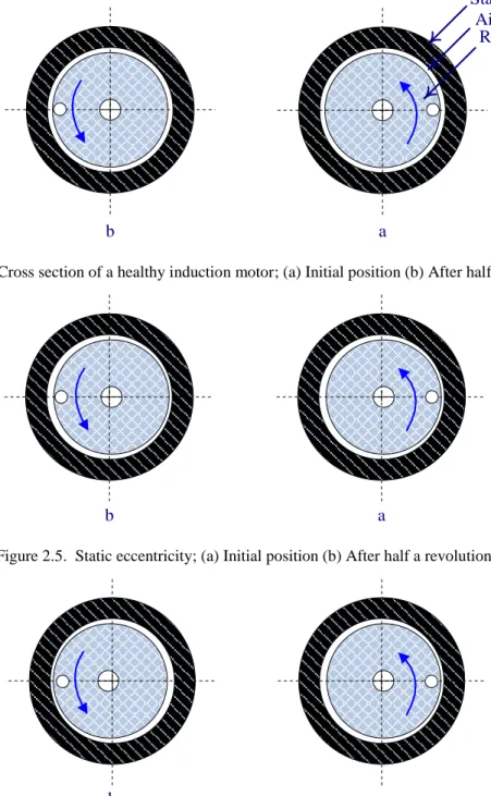
in vibration as the shaft dynamics are affected by the altered air gap. For static eccentricity the position of minimum radial air gap length is fixed in space while dynamic eccentricity is a function of space and time (see Figure 2. 4 to Figure 2.6 ).
Stator Rotor Air gap
b a
Figure 2. 4. Cross section of a healthy induction motor; (a) Initial position (b) After half a revolution.
b a
Figure 2.5. Static eccentricity; (a) Initial position (b) After half a revolution.
b a
CHAPTER-2 Literature review
12
2.2.3
Other Faults
A small number of failures in induction motors are linked to external factors. These faults can be caused by environmental, cooling, installation or manufacturing problems.
2.3
Fault detection Methods
There are numerous methods of induction motor fault diagnosis were developed in the last decades such as motor current signature analysis, temperature measurements, vibration monitoring, chemical analysis, artificial intelligence and stochastic optimisation techniques. These diagnostic methods may involve several different fields of science and technology.
2.3.1
Motor current signature analysis
MCSA is one of the most powerful methods of online fault diagnosis due to its low cost and simplicity [21]. Motor current signature analysis (MCSA) is based on current monitoring of an induction motor. The MSCA uses current spectrum of the machine for locating characteristic fault frequencies. Fast Fourier Transform and Wavelet transform are used to analyse motor current signature by identifying fault spectrum and extracting unique features for fault diagnosis.
Stator current contains unique fault frequency components that can be used for detection of various faults of motor. When a fault is present, the frequency spectrum of the line current becomes different from the healthy machine. The motor faults could be diagnosed through the comparison of recorded stator current signals and the reference signals in the frequency domain. MCSA can easily detect the common machine fault such as rotor fault, short winding fault, bearing fault, air gap eccentricity fault, etc [46, 47]. Schoen and et al. addressed the application of MSCA
CHAPTER-2 Literature review
13
for detection of rolling-element bearing damage [48].
2.3.2
Artificial Intelligence diagnoses
The main idea behind Artificial Intelligence (AI) is to mimic natural human intelligence in the form of a computer program to tackle problems that are hard to solve by traditional methods
2.3.2.1Neural Networks
Artificial neural networks are modelled on the neural connections in the human brain. Each artificial neuron accepts several inputs, applies preset weights to each input and generates a non-linear output based on the result. The neurons are connected in layers between the inputs and outputs. The application of artificial intelligence methods [49, 50], like neural networks, is rather easy to develop and to perform. Neural networks can be applied when the information about the process is obtained by measurements, which later can be used in the training procedures of neural nets. This method is an on-line technique and doesn’t use a mathematical model. Neural detectors can be designed using the data acquired from simulation or experimental tests [22].
2.3.2.2Fuzzy Logic
Fuzzy logic utilizes human knowledge by giving the fuzzy or linguistic descriptions a definite structure. A fuzzy logic approach may help to diagnose induction motor faults [51, 52]. In fact, fuzzy logic is reminiscent of human thinking processes and natural language enabling decisions to be made based on vague information. Fuzzy logic allows items to be described as having a certain membership degree in a set. This allows a computer, which is normally constrained to 1 and 0, to delve into the continuous realm.
CHAPTER-2 Literature review
14
2.3.3
Park’s Vector Approach
This method is based on the visualization of the motor current Park’s vector representation which is based on the identification of a specified current pattern obtained from the transformation of the three-phase stator currents to an equivalent two-phase system [53].
A healthy machine shows a perfect circle in Park’s vector representation while an elliptical pattern is observed if the machine is faulty. Park’s vector method can be used for diagnosing many types of induction motor faults such as air gap eccentricity, stator winding short-circuits, occurrence of rotor cage fractures, open wound rotor and bearing damages [54-56]. Cruz [53] has used Park’s vector approach to detect several types of rotor faults. The main advantage of this method is that the change in the shape of the line current phasor can be clearly observed, making it easy to diagnose machine faults. The main disadvantage is that it is not effective for load faults and broken rotor bar faults.
2.3.4
Stochastic optimisation search methods
These optimisation techniques depend on the idea of neighbourhood search and there is no mathematical model of the system involved. Heuristic techniques seek near optimal solutions without being able to guarantee either feasibility or optimality of the solution [57]. The principles of heuristic techniques are easy to understand, implement and use. The heuristic optimisation is very popular in applications. Every method uses a different search rule of finding optimal or near optimal solutions. The space of all feasible solutions is called the search space. Each and every point in the search space represents one possible solution. Therefore each possible solution is represented by one point in the search space. In effect, this technique searches through the solution space and moves in the direction of a known solution until a suitable solution is found or time bound is elapsed.
CHAPTER-2 Literature review
15
Many stochastic algorithms have been developed in recent years to address optimisation problems. The most popular algorithms are:
Genetic Algorithms (GA)
Ant Colony Optimisation (ACO)
Simulated Annealing (SA)
Particle Swarm Optimisation (PSO)
Tabu Search (TS)
Bacterial Forging Optimisation (BFO)
Many researchers have used these techniques; Zakaria [16] has used SA algorithm for induction machine fault detection. Ethny [58] has also used PSO and compare it with SA and BFO algorithms for induction machine fault identification. A tabu search algorithm has been used by Montane [59] for the vehicle routing problem. Cai [60] is applied GA for speed estimation of induction motor. In this study, GA, TS and SA algorithms were used because they are some of the most widely used algorithms and have proven to be very effective and robust in a wide range of applications. A brief description of the three algorithms used in this thesis is presented in the following subsection,
2.3.4.1Tabu search
Tabu Search (TS) is a new a stochastic optimisation procedure and has traditionally been used for optimisation problems [61]. TS has the power to avoid being trapped in local minima by using a tabu list. This tabu list constitutes the short-term memory which records any repeated solutions as a forbidden move. At each iteration, a set of candidate moves is extracted from the neighbourhood for evaluation and the best move is selected as a new solution. If the new solution is not tabu, it is accepted as a current solution, even if it is not a better solution. The tabu list is then updated with a new set of solutions. The advanced mechanisms of TS include the uses of intensification and diversification; by using the intensification mechanism, the algorithm does a more comprehensive exploration of attractive regions which may direct it to a local optimal point and by using the diversification mechanism, the
CHAPTER-2 Literature review
16
search is moved to previously unvisited regions to avoid cycling. This process of TS continues until the stopping criterion has been reached whereby the determined optimal solution for that specific problem is selected.
2.3.4.2Genetic Algorithm
Genetic algorithm (GA) is a stochastic search technique inspired by the mechanism of evolution, and natural selection. GA is successful at avoiding local minima and has been proven to be effective in solving difficult combinatorial optimisation problems. Traditional optimisation techniques use a single candidate and use repeated search techniques. However, the GA approach searches a population of candidates across several areas of a solution space simultaneously. The population consists of individuals or chromosomes which can be represented by strings of real or binary numbers. This population represents points in the solution space. The chromosomes evolve through successive iterations called generations. A new set of solutions, called offsprings, are created in a new generation. The basic operators in GA are selection, crossover and mutation. During each generation, the individuals are evaluated according to their objective and fitness functions. Following several generations, the algorithm then converges to the best chromosome that represents the optimal or near optimal to the problem.
2.3.4.3Simulated Annealing
Simulated annealing (SA) is an optimisation technique which has been widely used in large combinatorial optimisation problems. SA mimics the annealing process for crystalline solids. The annealing process starts with melting the solid by heat treatment and slowly decreasing the annealing temperature. The SA algorithm views the cost function being minimised as equivalent to the energy state of a physical system, and the process of reaching equilibrium is equivalent to repeatedly accepting or rejecting changes in energy from one state to another. The algorithm starts from a randomly generated initial point and simulates a walk through the solution space; a candidate configuration is accepted if its cost is less than the current configuration,
CHAPTER-2 Literature review
17
while deteriorating steps are only accepted with a certain probability. As the temperature parameter is decreasing, the algorithm accepting only good solutions until converges to a solution very close to optimality [62].
2.4
Summary
The most prevalent faults in induction motors are described in this chapter. The use of electric motors is becoming ever more common in various industries, resulting in an increased demand for fault detection methods. This chapter has provided a general review of existing induction motor fault detection methods. Relevant information about stochastic search algorithms used in this study has also been presented. In the next chapter, the three stochastic algorithms (Genetic Algorithms, Tabu Search and Simulated Annealing) will be explained in more details.
CHAPTER-3 Stochastic optimisation algorithms 18
CHAPTER 3
STOCHASTIC OPTIMISATION
ALGORITHMS
3.1
Introduction
This chapter introduces the concepts involved in the various stochastic optimisation algorithms (SOA) that have been investigated. Optimisation problems are defined by a set of solutions and an objective function associated with each solution. The goal when addressing an optimisation problem is to optimise the objective function to find solutions that are optimal or near-optimal in a reasonable amount of time. Conventional optimisation methods suffer from the problem of local minima trapping. This problem can be circumvented by using stochastic optimisation methods such as Genetic Algorithm (GA), Simulated Annealing (SA) and Tabu Search (TS). Many efforts have been directed toward developing efficient heuristic algorithms. SOA have been applied to a wide variety of combinatorial optimisation problems with great success. Several stochastic search techniques have been proposed in the literature. Figure 3.1 shows a simple classification of some stochastic optimisation methods according to their algorithmic structure [63]. In this work, three standard stochastic optimisation methods: genetic algorithm, tabu search and simulated annealing are used to identify induction machine winding faults. These stochastic algorithms are implemented using the MATLAB language on a PC. When using stochastic algorithms, the search process is repeated until a stopping criterion has been reached. There are various kinds of termination conditions such as
CHAPTER-3 Stochastic optimisation algorithms
19
the use of a fixed number of iterations, fixed number of generations, fixed amount of time, when the objective value reaches a pre-specified value, or when there is no improvement of the objective function. The simplest form of stopping criterion is a fixed number of iterations or generations. The search is terminated once a preset maximum number of iterations have been reached. The best solution found in this period will be the result of the search.
Stochastic Optimisation Algorithms Random Optimisation Simulated Annealing Tabu Search Evolutionary Computation Stochastic Hill Climbing Evolutionary
Algorithms Swarm Intelligent
Ant Colony Optimisation Particle Swarm Optimisation Genetic Algorithms Bacterial Foraging
Figure 3.1. Classification of stochastic optimisation algorithms [63].
CHAPTER-3 Stochastic optimisation algorithms
20
3.2
Genetic Algorithm
3.2.1
Introduction
Genetic algorithm (GA) is a stochastic search technique inspired by the mechanisms of evolution and natural selection. Like other evolutionary algorithms, GA is a population-based metaheuristic* optimisation algorithm that uses biology-inspired mechanisms such as mutation, crossover, natural selection and survival of the fittest (Figure 3.2). GA was introduced in 1975 by a team led by John Holland and was later developed by De Jong Goldberg and many other researchers. There are many different GA algorithms but the basic idea, which is based on Darwin’s theory of survival of the fittest, is the same [64, 65]. GA is successful in avoiding local minima and has proved to be effective in solving difficult combinatorial optimisation problems. GA is efficient, reliable and robust. It finds widespread applications in system optimisation problems in science, economy and many other fields. GA has been successfully applied to numerous combinatorial problems such as the travelling salesman problem [66], scheduling problems [67], graph colouring [68] and many others. Traditional optimisation techniques use a single candidate and repeated search techniques. The GA approach on the other hand searches a population of candidates across several areas of a solution space simultaneously. The population consists of individuals or chromosomes which can be represented by strings of real or binary numbers. GA uses fitness functions for evaluation rather than derivatives. This technique is generally able to find the optimal or near-optimal solutions to the considered optimisation problems. One of the drawbacks of GA is their complex computational requirements as they can be very slow in some applications. This problem can be overcome by using faster computers. Sastry et al. give a good introduction to genetic algorithms [69]. In this section, the basic principle of genetic algorithm is described, followed by a simple example showing the use of a genetic algorithm to find the optimum parameters of a given problem.
* The term metaheuristic derives from the composition of two Greek words: heuristic means “to find” while the prefix meta means “beyond, in an upper level.” It refers to the set of strategies that guide the iterative search process.
CHAPTER-3 Stochastic optimisation algorithms
21
Figure 3.2. The basic cycle of Evolutionary Algorithms.
3.2.2
Basic concept of genetic algorithm
In Genetic Algorithm only two kinds of operations are executed: evolutionary operations (selection) and genetic operations (crossovers and mutations). The GA starts with a random population of potential individuals, each representing one possible solution to the problem. A population is made up of a set of individuals, and evolution from one generation to the next takes place by the deletion of existing individuals and the creation of new ones. During each generation, the individuals are evaluated according to the objective and fitness functions. After obtaining the fitness of all individuals, a selection process is used to choose individuals for reproduction. Individuals with higher fitness should have a higher probability of being selected as parents so that the more successful individuals will have more chances to mate and generate offspring. The least fit individuals in each population are then replaced by the offspring so that the population size remains constant and another generation starts. Through an iterative process, the population evolves towards better regions of the search space. After many generations, the algorithm reaches convergence towards the best chromosome, or the individual which signifies the optimal solution or the nearest optimal solution to the problem [70]. The algorithm stops once the termination criteria is met. These processes are described in more detail in the following subsections. The basic steps of simple genetic algorithm can be described as follows: Initial Population Evaluation Selection Reproduction Fitness Assignment
CHAPTER-3 Stochastic optimisation algorithms
22 Step 1: Generate an initial population randomly.
Step 2: Evaluate the fitness value of each individual in the population.
Step 3: Select parent individuals from a population that have higher fitness values to generate new offspring.
Step 4: Crossovers and mutations are applied to the selected offspring. Step 5: Replace the worst part of the population by new offspring.
Step 6: If the stopping criterion has been reached, stop; otherwise save the best solution and proceed to Step 2.
Figure 3.3 shows the flowchart for the GA algorithm.
Figure 3.3. GA flowchart. N
Gen = 0
Evaluate Fitness Value Selection Gen >MaxGen Crossover Mutation Gen = Gen+1 Retrieve Results Stop
Create Initial Population
Start
Insert New Offspring into New Population
CHAPTER-3 Stochastic optimisation algorithms
23
3.2.2.1Initialisation
To start the GA algorithm, a specified number of individuals, a maximum number of generations and the type of chromosome coding are chosen. The chromosomes are encoded as either binary or real numbers. However, by using binary strings, the chromosomes may become long, due to the number of digits that may be required to form one single variable. By using real numbers, the chromosome length is reduced and becomes easier to understand, as each allele or gene of the chromosome or individual is represented by its real value. The initial set of random solutions is known as the initial population. The number of individuals in the population is called the population size which is usually recommended to be between 30 and 100 [71]. It has been noted that too large a population slows down the optimisation, while a small population does not utilise the genetic operators effectively. The crossover and mutation rates for the reproduction function should also be defined as should the selection method.
3.2.2.2Objective function and fitness functions
The objective function is a function associated with an optimisation problem that would determine the merit of the solution. For example, the function indicates that the best individuals would be the ones with the lowest value of objective function in the problem of minimisation and vice versa in the case of maximisation. Every individual in the population has its gene representation, called its code, and performance evaluation, called its fitness value; the fitness calculation is a measure of how good a particular solution to the problem is, so that different solutions can be compared based on the values obtained from the fitness function. This means that individuals with higher fitness value will have higher probability of being selected as candidates for the next generation.
3.2.2.3Selection
CHAPTER-3 Stochastic optimisation algorithms
24
solutions) for generating offspring. This process is based upon their fitness values. This is achieved by assigning better solutions a higher probability of being chosen for recombination. It is also very important to allow a few less-fit individuals to increase the diversity of the population. A number of different selection strategies have been implemented in different algorithms including roulette wheels, local tournaments, various ranking schemes, etc. A simple reproduction operator is the roulette wheel selection where each individual in a population has a roulette wheel slot sized in proportion to its fitness; for example, if there are five individuals in the population with fitness values of 9, 3, 6, 5 and 8, the corresponding probabilities for these individuals are 29.03%, 9.68%, 19.35%, 16.13% and 25.81%, respectively. Figure 3.4 shows the selection probability for the 5 individuals. Individual 1 is the most fit individual and occupies the largest interval, whereas individual 2 is the weakest and correspondingly occupies the smallest interval. In order to select an individual, a random number is generated within the range (0, Sum). The variable Sum is determined as the sum of the row fitness values over all the individuals in the current population [72]. The individual whose segment of the wheel spans the number is selected. This process is repeated several times until the required number of individuals has been selected with the selection probability of an individual being proportional to its fitness value [73].
Figure 3.4. An example of roulette wheel selection.
4 3 1 5 5 1
Individual Selected probability 1 29.03% 2 9.68% 3 19.35% 4 16.13% 5 25.81% 2
CHAPTER-3 Stochastic optimisation algorithms
25
3.2.2.4Crossover
The process of crossover, which represents mating (recombination) of two parent individuals, is carried out by exchanging parts of their chromosomes to create new offspring. Each offspring shares genes with its parents. The process of crossover is applied with a certain probability referred to as the crossover rate. The crossover rate generally ranges from 0.25 to 0.95. The crossover operation is necessary to ensure convergence of the GA to an optimal solution. After selecting a pair of parents, the algorithm implements crossover only if a randomly generated variable is greater than the crossover rate, otherwise, the parents remain unchanged. Each offspring inherits genes from its parents. This is achieved by slicing the chromosomes and crossing over their genes. The simplest and most popular implementations of this process are one-point crossover and two-point crossover where the chromosome string of each parent organism is randomly split at one or two points, respectively. The crossover point is chosen at random in the range of [1, Lst -1] where Lst is the length of the
string. To generate new offspring using one-point crossover, a cut point is chosen randomly and the genetic information to the left of the cut of point in parent A are combined with the genetic information to the right of the cut of point in parent B. A second offspring can also be generated by using the right hand side string of parent A with the left hand side string of parent B. For a two-point crossover, two cut of points are set randomly and the section between the two points is taken from one parent and combined with the outer sections from the other parent. In the following example, the crossover point is set after the second bit in the case of one-point crossover. In the case of two-point crossover, the two crossover points are set after the second and fifth bits respectively. This operation is illustrated in Figure 3.5.
CHAPTER-3 Stochastic optimisation algorithms 26 0 0 0 1 0 0 1 0 1 1 1 1 0 0 0 1 0 0 1 0 1 1 1 1 0 0 1 1 1 1 1 0 0 1 0 0 0 0 1 1 1 0 1 0 0 1 0 1
One point crossover
Two point crossover
Crossover point
Before Mutation After Mutation
Before Mutation After Mutation
Figure 3.5. The GA crossover operation.
3.2.2.5Mutation
Mutation takes place by randomly changing a few bits in the chromosome of the resulting offspring. This prevents the solutions from falling into a local optimum and can also help in exploring new regions of the solution space. The mutation operation does not occur as frequently as the crossover function. This is achieved by using a low mutation probability (a value fixed throughout the whole search process) that represents how often parts of a chromosome will be mutated. First, the mutation point is selected randomly (Figure 3.6). After mutation, the resulting solutions become the current population. In the case of binary encoding, mutation is simulated by flipping bits at random, using a low probability in the range [0.001- 0.05]; for this work, a mutation probability of 0.05 was chosen. A gene can be mutated by swapping its value from 0 to 1 or 1 to 0. For real-value encoding, the mutation operator can be implemented by random replacement (i.e., the original value is replaced with a new randomly generated value). An illustration of the process of mutation in GA is shown in Figure 3.6. The mutation operator is more important at the final stages of the optimisation process when the majority of the individuals in the population possess similar qualities.
CHAPTER-3 Stochastic optimisation algorithms 27
1
0
0
1
1
1
1
0
1
0
1
0
0
0
1
1
1
0
1
0
Mutation Point Original Chromosome Mutated ChromosomeFigure 3.6. Illustration of mutation in Genetic Algorithms.
3.2.3
Reinsertion
The fitness of the new individuals is determined once a new population has been produced. A generation gap may occur where fewer individuals are produced and this may cause a difference between the old and new population sizes. Some of the new individuals need to be reinserted in the old population to maintain the original population size.
3.2.4
Application of GA to simple example
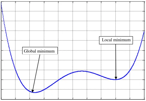
In this Section, the GA algorithm was implemented using Matlab on the following function (Equation 3.1) which has one global minimum of (0.846) at x = 2.388 as can be seen in Figure 3.7.
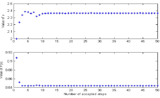
4150 . 5 9426 . 4 7927 . 1 2473 . 0 0116 . 0 ) (x x4 x3 x2 x f (3.1) The task of the GA algorithm is to optimise the variable x to minimise the objective function and to confirm the ability of GA to avoid becoming trapped in the local minimum of 1.5 at x = 8. The search range for variable x is set from -20 to 20. The Matlab code for this exercise is given in Appendix A1. Figure 3.8 shows that the GA
CHAPTER-3 Stochastic optimisation algorithms
28
algorithm terminates after 50 generations at the global minimum. The computational time was 1.965 sec and the value of x is 2.388.
Figure 3.7. Function with a local minimum.
Figure 3.8. Value of potential solution and objective function obtained by GA.
0 1 2 3 4 5 6 7 8 9 10 0.5 1 1.5 2 2.5 3 3.5 4 4.5 5 5.5 parameter (x) fu n c ti o n f (x ) Global minimum Local minimum