Continuous Speech Recognition by Neural Networks

(1)

doc. Ing. Jan Janoušek, Ph.D.

Head of Department doc. RNDr. Ing. Marcel Jiřina, Ph.D.Dean

ASSIGNMENT OF BACHELOR’S THESIS

Title: Continuous Speech Recognition by Neural Networks Student: Adam Zvada

Supervisor: Ing. Miroslav Skrbek, Ph.D.

Study Programme: Informatics

Study Branch: Computer Science

Department: Department of Theoretical Computer Science

Validity: Until the end of summer semester 2018/19

Instructions

Explore possible methods for continuous speech recognition using neural networks. Consider recurrent neural networks and the possibility of using neural Turing machines. Based on the investigation and in agreement with the supervisor, select the appropriate solution for the robot NAO. Benefit from existing libraries providing implementations of the required methods. Validate the proposed solution on real data. Specify the scope of the work, together with the supervisor.

References

(2)

(3)

Czech Technical University in Prague Faculty of Information Technology Department of Theoretical Informatics

Bachelor’s thesis

Continuous Speech Recognition by Neural

Networks

Adam Zvada

(4)

(5)

Acknowledgements

I would like to express my very great appreciation to my supervisor Ing.

(6)

(7)

Declaration

I hereby declare that the presented thesis is my own work and that I have cited all sources of information in accordance with the Guideline for adhering to ethical principles when elaborating an academic final thesis.

I acknowledge that my thesis is subject to the rights and obligations stip-ulated by the Act No. 121/2000 Coll., the Copyright Act, as amended, in particular that the Czech Technical University in Prague has the right to con-clude a license agreement on the utilization of this thesis as school work under the provisions of Article 60(1) of the Act.

(8)

Czech Technical University in Prague Faculty of Information Technology

c

This thesis is school work as defined by Copyright Act of the Czech Republic. It has been submitted at Czech Technical University in Prague, Faculty of Information Technology. The thesis is protected by the Copyright Act and its usage without author’s permission is prohibited (with exceptions defined by the Copyright Act).

Citation of this thesis

Zvada, Adam. Continuous Speech Recognition by Neural Networks. Bach-elor’s thesis. Czech Technical University in Prague, Faculty of Information Technology, 2018.

(9)

Abstrakt

Tato bakaláˇrská práce se zamˇeˇruje na oblast rozpoznáván´ı ˇreˇci s pomoc´ı neu-ronových s´ıt´ı a klade si za c´ıl implementovat ”end-to-end” rozpoznávaˇc ˇreˇci jako hlasové uˇzivatelské rozhran´ı pro robota NAO.

Uvaˇzovaná architektura rozpoznávaˇce ˇreˇci je sloˇzena ze tˇr´ı d˚uleˇzitých ˇcást´ı: extrakce pˇr´ıznak˚u signálu ˇreˇci za pouˇzt´ı metody mel-frekvenˇcn´ıch kepstráln´ıch koeficient˚u, rozpoznávaˇce v podobˇe rekurentn´ı neuronové s´ıtˇe s ”long-short-term-memory” buˇnkami a algoritmu ”connection temporal classification” k z´ıskán´ı finaln´ıho pˇrevedeného textu.

Výsledkem této práce je ”end-to-end” rozpoznávaˇc ˇreˇci, natrénovaný na VCTK korpusu a implementovaný v programovac´ım jazyce Python s vyuˇzit´ım knihovny hlubokého uˇcen´ı TensorFlow.

Kl´ıˇcová slova neuronové s´ıtˇe, rekurentn´ı neuronové s´ıtˇe, rozpoznáván´ı ˇreˇci, TensorFlow, CTC, LSTM, Robot NAO, Python

Abstract

The aim of this bachelor thesis is to explore the field of speech recognition using neural networks with a goal to implement end-to-end speech recognizer as voice-user interface for robot NAO.

(10)

The proposed speech recognizer architecture is consisted from three main components: feature extraction of speech signal using mel-frequency cepstrum coefficients method, recognizer as recurrent neural networks with long-short-term-memory cells, and connection temporal classification algorithm for pre-dicting the final transcription.

The result of this work is end-to-end speech recognizer trained on VCTK corpus and implemented in programming language Python, using deep learn-ing library TensorFlow.

Keywords neural networks, recurrent nerual networks, speech recognition, TensorFlow, CTC, LSTM, Robot NAO, Python

(11)

List of Figures

1.1 Illustration of nerve cell and communication flow . . . 4 1.2 Illustration of nerve cell and communication flow . . . 5 1.3 Basic topology of fully connected artificial neuron network with

input vector of size 3, output vector of size 2 and two hidden layers. 7 2.1 Simple RNN topology and illustration of unrolled RNN through

time[40] . . . 11 2.2 Deriving the gradients according to the backpropagation through

time (BPTT) method. Notation for output value(t) corresponds to ouryt[24]. . . 13 2.3 Situation of using gradient clipping (dashed line) against the

ex-ploding gradient [28] . . . 14 2.4 Diagram of LSTM cell [16]. . . 15 3.1 Basic building blocks of a Speech Recognizer [38] . . . 19 3.2 Illustration of raw speech signal from wav file with sampling

fre-quency of 8kHz [11] . . . 20 3.3 Steps of MFCC [30] . . . 21 3.4 Vector of Mel Frequency Cepstral Coefficients through time. . . . 22 3.5 Diagram of traditional speech recognizer . . . 23 3.6 End-to-end speech recognizer diagram using CTC [26] . . . 24 4.1 Speech Recognition System . . . 25 4.2 Diagram of the learning phase for the speech recognition system . 26 4.3 Robot NAO . . . 31 5.1 Configuration of hyperparameters . . . 34 5.2 Learning Error rate on Digits for configuration on Figure 5.1 . . . 35 5.3 Configuration of hyperparameters . . . 35 5.4 Learning Error rate on Digits for configuration on Figure 5.3 . . . 36 5.5 Configuration of hyperparameters . . . 36

(14)

5.6 Learning Error rate on VCTK for configuration on Figure 5.5 . . 37 5.7 Continuation of Learning Error rate on VCTK for configuration on

Figure 5.5 with dropout reduced to 0.5 . . . 37

(15)

Introduction

The problem of speech recognition (SR) has been an important research topic since as early as the 70s. Recently, the field of SR has seen major advances because of the rise of computing power (GPUs) which allowed innovation in machine learning and artificial intelligence algorithms. Now we have access to voice control through speech recognition in mobile devices, computers, smart TVs or even fridges.

Before the emergence of deep learning, researchers often utilized other classification algorithms such as Hidden Markov Model (HMM) with many complex handcrafted components. The field is now gradually moving towards end-to-end speech recognizer using just neural networks which learns to tran-scribe an audio sequence signal directly to a word sequence, one character at a time. Therefore, all the handcrafted components would be replaced with a just one learning model.

In this thesis, we present the concept of artificial neural networks (ANN), basics of the internal network architecture and explained the training phase of ANN. We extend the knowledge of neural networks by introducing recurrent neural networks and most importantly we cover how speech recognition system works and how can we build end-to-end SR using neural networks.

Our goal is to get theoretical overview in this field and implement end-to-end speech recognizer using neural networks and TensorFlow library which would be used in Robot NAO as voice-user interface on Robot NAO.

(16)

(17)

Chapter

1

Neural Network

Neural networks have a remarkable ability to derive meaning from complicated data. They can be used to extract patterns and detect trends that are too complex to be noticed by either humans or other computer techniques [33]. Even though they have been around since the 1950s, it is only in the last decade when they started to outperform robust system or even humans in specify tasks. However, they require a huge amount of training examples and computational power to be trained for preforming a reasonable prediction. Fortunately, GPUs has seen enormous increase in performance1 and 90% of the data in the world today has been created in the last two years alone, at 2.5 quintillion bytes of data a day [18]. That’s why ANN is big topic in Computer Science and in the technology industry and it currently provides the best solutions to many problems such as speech recognition, image recognition, and natural language processing.

1.1 Inspiration in Nature

Artificial neural network (ANN) is heavily inspired by the way how biological neural networks process information in the human brain. Even though our brain is extremely complex and still not fully understand, we just need to know how information is being transferred. The basic building block is nerve cell called neuron. It receives, processes, and transmits information through electrical and chemical signals [27]. It’s estimated that an average human has 86 billion neurons [9].

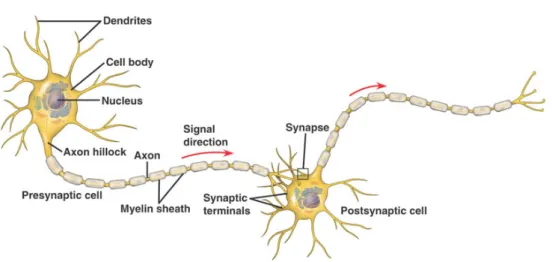
As shown on Figure 1.1,dendrites are extensions of a nerve cell that prop-agate the electrochemical stimulation received from other neurons to the cell body. You may think of them as inputs to neuron, whereas neuron’s output is called axon, a long nerve fiber that conducts electrical impulses away from

1

GPUs are explicitly designed to handle multiple matrix calculations at the same time. Evaluation and training of artificial neural networks are mostly matrix operations.

(18)

1. Neural Network

Figure 1.1: Illustration of nerve cell and communication flow

the cell body. The end of axon is branched to many axon terminals which can be again connected to other dendrites. The connection is managed by

synapses that can permit the passing of electrical signal to cell body. Once the cell reaches a certain threshold, an action potential will fire, sending the electrical signal down the axon to other connected neurons.

1.2 Artificial Neuron

Artificial neuron is a generic computational unit, basic building block for artifi-cial neural network (ANN). It’s simplified version of the biological counterpart and we can map parts of biological neuron with the artificial one. It takesn in-puts represented as a vectorx∈_Rn_{which correspond to dendrites. Generally} artificial neuron produces single output y ∈Ras biological neuron where we

call it axon. Each neuron’s inputi= 1,2, . . . , nhas assigned weight (synapse)

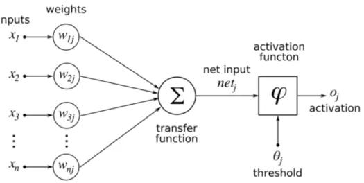
w1, w2. . . wn, they refer to the connection strength between neurons. Weights and same as for synapse are the backbone of learning because in training phases, they keep changing to produce wanted output. Inside the artificial neuron, input vector with their weights are combined and run through an activation function producing some output y. This process is illustrated in Figure 1.2.

1.3 Perceptron

Perceptron is the simplest ANN with just one neuron and since we covered the basic intuition about artificial neuron we may proceed further and take a look at how output is actually calculated. The equation for a perceptron can 4

(19)

1.3. Perceptron

Figure 1.2: Illustration of nerve cell and communication flow

be written as y=f( N X i=1 wi·xi+b) (1.1) where • x - input vector • y - predicted output • f - activation function • w - weights • b - bias

Perceptron is a basically linear classifier, therefore the data has to be lin-early separable otherwise we would not be able to make the correct prediction. Problems such as speech recognition are not definitely linearly separable, how-ever we can solve non-linear decisions for example by introducing another layer of neurons, thus creatingMultilayered Perceptron.

1.3.1 Activation Functions

We have stated that biological neuron fires electrical signal to other connected neurons whenever it reaches a certain threshold of incoming electrical im-pulses. Activation function is based on that concept and inside an artificial neuron it is used for calculating output signal via equation 2.1. It introduces non-linear properties to our ANN and without an activation function would

(20)

1. Neural Network

be just a regular linear regression model. Nowadays many different activation function are being used and their performance varies from model to model. List of some activation function:

• Sigmoid σ(x) = 1 1 +e−x • Hyperbolic Tangent tanh(x) = (e x₋_e−x₎ (ex₊_e−x₎ • ReLU f(x) = ( 0 forx <0 x forx≥0 • Softmax fi(~x) = exi PJ j=1exj , i= 1,2. . . J

whereiis number of output

1.3.2 Bias

We can think of bias as a value stored inside neuron and being used to calculate its output. The bias value allows the activation functions to be shifted to the left or right, to better fit the data.

1.4 Topology of Artificial Neuron Network

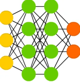
Basic ANN as feedforward model is a directed graph with nodes as neurons and edges with weights representing connection to other neurons. ANN can be divided to three important layers as shown in Figure 1.3. Yellow nodes is an input layer which takes input data, dimension of input vector has to correspond to number of input nodes. Hidden layer as the green nodes is most important to ANN and that is where the training and evaluation happens. Number of hidden layers and neurons needs to be in a good ratio between its size and its effectiveness. Output layer produces output vector as the prediction for given input.

1.4.1 Network Evaluation

ANN are sometimes called feedforward neural network. The reason behind is that the input is fed into the neuron and then forward to another layer, thus ANN are evaluated layer by layer. All neurons calculate the output using similar formula as Perceptron 2.1.

(21)

1.5. Training

Figure 1.3: Basic topology of fully connected artificial neuron network with input vector of size 3, output vector of size 2 and two hidden layers.

1.5 Training

The greatest trait of ANN is ability to learn from given data and then make the best approximate prediction. The aim of the learning process is to find the most optimal values for network’s weights and biases while minimizing error on predicated values. For ANN to learn we have to introduce training data consisted of input vector which will be fed to the network and desired output value (label) for calculating our loss. This approach is called super-vised learning2.

1.5.1 Loss Function

Loss function compares the prediction from ANN with the desired output and returns the error of the prediction. During a training ANN, the goal is to minimize given loss function. The most common and most intuitive loss function is Mean Squared Error (MSE),

MSE(y,yˆ) = 1 n n X i=1 (yi−yˆi)2. 1.5.2 Backpropagation

Backpropagation algorithm is responsible for the ability to learn from given training data. It is an iterative algorithm which for each training data from

(22)

1. Neural Network

given training dataset backpropagates the error and adjust the weights and biases accordingly to get desired output.

1.5.2.1 Optimization

Backpropagation requires optimizer to minimize the error on the training data. We will describe backpropagation with using gradient descent as the most common optimization algorithm.

Weights and biases are updated using formula,

W_jkl :=W_jkl −α ∂ E ∂Wl jk bl_j :=bl_j −α∂ E ∂bl j (1.2)

where W_jkl is weight with connection between unitj in layer l and unit i in layerl+ 1,bl_j is bias associated with unitiin layer l+ 1,α is a learning rate [42], and _∂W∂ El

jk

or ∂ E_∂bl j

can be interpreted as minimizing loss function with respect to given weight and bias respectively.

By applying a chain rule twice on the partial derivative of the loss function with respect to a weight, we get

∂ E ∂Wl jk = ∂ E ∂al j ∂ al_j ∂zl j ∂ z_jl ∂Wl jk (1.3)

wherez_jl is a sum of weighted inputs to unitj in layer l

zl_j =bl_j+ K X

k=1

wl_jkal_k−1 (1.4)

and al_j is an output of nodej in layer l

al_j =f(z_jl). (1.5)

Let’s calculate the last two products of equation 2.3:

∂ al_j ∂z_jl =f 0₍_zl j) ∂ z_jl ∂W_jkl = ∂ W_jkl al_k ∂Wjkl =al_k−1 (1.6)

We introduce a new variableδ_jl which represents the error in unitj in layerl

and helps us to better understand and calculate real interested value of ∂ E ∂Wl jk and _∂b∂ El j . δ_jl = ∂ E ∂zl j (1.7) 8

(23)

1.5. Training

We will simplify the error equation on neuron j in output layerL as

δ_jL= ∂ E ∂z_jL = ∂ E ∂aL_j ∂ aL_j ∂z_jL = ∂ E ∂aL_j f 0₍_zL j) (1.8)

Now we have enough information to reformulate equation 2.3 for output layer to

∂ E ∂W_jkl =δ

L

kaLj. (1.9)

However, to be able to update weights inside the hidden layers, we have to redefine the calculation ofδl

j. We know that the error produced by an output neuron is just influencing the output value but inside a hidden layer the pro-duced error propagates to all following layers. Therefore, we have calculate theδl_j where layerlis inside a hidden layer and take into account allδl+1from following layer l+ 1. δ_jl = ∂ E ∂zl j =X i ∂ E ∂z_il+1 ∂ z_il+1 ∂zl j =X i ∂ E ∂z_il+1 ∂ z_il+1 ∂al j ∂ al_j ∂zl j =X i δ_il+1W_ijl+1f0(z_jl) (1.10) where the sum index iiterates over all neurons in layerl+ 1 and Notice that we have substituted ∂ E

∂z_il+1 withδ l+1

i which is calculated from previous iteration [32].

Finally, we may calculate all weights adjustments through the whole network as W_jkl :=W_jkl −αδl_kal_j (1.11) where δ_kl = ∂ E ∂aL j f0(z_jL), l=L (1.12) or δ_kl =X i δ_il+1W_ijl+1f0(z_jl), l= 2, . . . , L−1. (1.13) We won’t be exampling the equation for biases adjustments because it follows a similar process shown above with just little changes, resulting to equation

bl_j :=bl_j−αδ_lj (1.14)

1.5.2.2 Backpropagation Algorithm Backpropagation algorithm in pseudocode:

(24)

1. Neural Network

Algorithm 1 Backpropagation

1: Initialize network weights and biases

2: for eachtraining data from training dataset do

3: Forward pass and calculate network prediction for given training input

4: Calculate error δL for output layer

5: Calculate errorsδl for hidden layers

6: Update weights and biases using precalculated δl

(25)

Chapter

2

Recurrent Neural Network

Neural networks are powerful learning models that achieve state-of-the-art results in a wide range of machine learning tasks. Nevertheless, they have limitations in the field of sequential data. Standard ANNs rely on the as-sumption of independence among the training examples but if data points are related in time or space then ANNs would not be the right model for the task [23].

Recurrent neural network (RNN) is type of neural network which is precisely designed to work with sequential data through time. The key difference is that RNN’s neurons in hidden layer have a special edge (recurrent edge) to a next time step which can be interpreted as a loop. In RNN, the neuron’s output is dependent on the previous computations which is sent through the recurrent edge. Basically, the recurrent edges or loops allow persistence of information from one time step to the next one as shown on Figure 2.1 [12].

Figure 2.1: Simple RNN topology and illustration of unrolled RNN through time[40]

(26)

2. Recurrent Neural Network

2.1 Evaluation

In 2.1 we may see simplification of evaluation process of RNN through the time steps. RNN’s neuron cell in hidden layer takes two inputs, xt and ht−1

which is value (hidden state) sent through the recurrent edge from previous time-step. The cell also produces two outputs,htas hidden state for upcoming time-step

ht=f(Whxxt+Whhht−1+bh)

wheref is arbitrary non-linear activation function, Whx is matrix of conven-tional weights, Whh is the matrix of recurrent weights and bh is a bias. The second output from cell isytwhich outputs the predication using precalculated hidden stateht,

yt=Whyht+by whereWhy is matrix of output weights.

2.1.1 Softmax Fucntion

It is very common for RNN models to usesoftmax as activation function for output layer. Softmax function helps to get probability distribution of outputs so it’s useful for finding most probable occurrence of output with respect to other outputs. softmax(y)j = ezj PK k=1ezk , forj= 1, . . . , K

Softmax is being used for calculating output value of ytresulting to formula

yt= softmax(Whyht+by).

2.2 Training

Training a RNN is similar to training a traditional ANN. We also use the backpropagation algorithm, but since the parameters are shared by all time-steps in the network, the gradient at each output depends not only on the calculations of the current time-step, but also the previous time-steps [6].

2.2.1 Backpropagation Through Time

The most used algorithm to train RNN isbackpropagation through time (BPTT), introduced by Werbos in 1990 [36]. BPTT is basically an extended version of backpropagation algorithm where we not only propagate the error to all following layers but also through the hidden states. We may think of it as unrolling the RNN to sequence of identical ANNs where the recurrent edge connects the sequences of neurons in hidden layer together as shown on Figure 12

(27)

2.2. Training

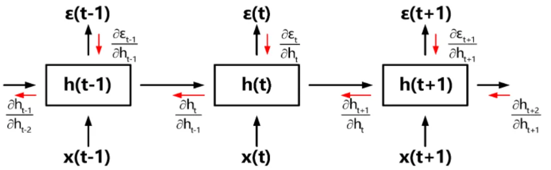
Figure 2.2: Deriving the gradients according to the backpropagation through time (BPTT) method. Notation for output value (t) corresponds to our

yt[24].

2.1 and 2.2. On Figure 3.2 2.2 is also indicated how the errors are propagated. The propagation of errors through hidden states allows the RNN to learn long term time dependencies. The calculated gradients of the loss function for de-fined parameter (W, b) through the sequence of unrolled RNN are then sum up, producing the final gradient for updating the weights or biases.

∂ E ∂Wijl = T X t=1 ∂ Et ∂Wijl where E is predefined loss function, Wl

jk is weight with connection between unit j in layer l and unit i in layer l+ 1, T is number of input sequences and ∂ Et

∂Wl ij

is calculated similarly as in backpropagation with just considering existence of recurrent edges

∂ Et ∂Wl ij = t X k=1 ∂ Et ∂yt ∂ yt ∂ht ∂ ht ∂hk ∂ hk ∂Wl ij To compute the ∂ ht

∂hk we use simple chain rule over all hidden states in interval

[k,t]. ∂ ht ∂hk = t Y i=k+1 ∂ hi ∂hi−1

Putting equations together, we have the following relationship [28].

∂ E ∂W_ijl = T X t=1 t X j=1 ∂ Et ∂yt ∂ yt ∂ht ( t Y i=k+1 ∂ hi ∂hi−1 ) ∂ hk ∂W_ijl 2.2.2 Exploding and Vanishing Gradients

Even though, RNNs had achieved success in learning short-range dependen-cies, they haven’t been showing any worth mentioning achievement with

(28)

learn-2. Recurrent Neural Network

ing mid-range dependencies. That was mainly cause by problems ofvanishing

and exploding gradients, introduced in Bengio in 1994 [4].

The exploding gradient problem occurs when backpropagating the error across many time steps, that could lead to exponentially grow of gradient for long-term components. Basically, a small change in parameters at initial stages can get accumulated through the time-steps resulting to the exponen-tially grow. The values of weights can become so large as to overflow and result inNaN values.

The vanishing gradient problem refers to opposite behavior when the gra-dient values are shrinking exponentially fast and eventually vanishing com-pletely. Gradient contributions from later time-steps become zero and the states at those steps doesn’t contribute so we end up not learning long-range dependencies. Vanishing gradients aren’t exclusive to RNNs, they also happen in deep ANN[7].

2.2.2.1 Solutions

To overcome problem with exploding gradient we can applygradient clipping

method. The values of the error gradient are checked against a predefined threshold value and clipped or set to that threshold value if the error gradient exceeds the threshold [1]. Another possibility is to use ReLU activation

Figure 2.3: Situation of using gradient clipping (dashed line) against the ex-ploding gradient [28]

function which tends to reduce the the exploding gradient problem. To fix the problem of vanishing gradient is little more complicated. We can always try perform more careful initialization process but it does not always help. It requires different architecture approach achieved by updating the RNN neuron to more complex LSTM cells.

(29)

2.3. LSTM

2.3 LSTM

Long-Short-Term-Memories (LSTM) is special kind of RNN cell, introduced by Hochreiter and Schmidhuber in 1997 [15]. Conventional RNNs are only just able to learn short-term dependencies because of vanishing gradient problem. However, LSTM does not get effected and it’s capable of learning long-term dependencies.

Figure 2.4: Diagram of LSTM cell [16].

As shown on Figure 2.4 we notice that LSTM is just more complex acti-vation units. Similarly, as basic RNN cell which propagates hidden state of

htto another time-step and also as cell output, the LSTM cell has extra state denoted as ct and called cell state and it’s just being propagated to another time-step. The cell state is more of a cell’s memory.

LSTM architecture follows stages during the evaluation where first we have to decide what information we want to get rid of from cell state, that is achieved applying formula using sigmoid function

ft=σ(Wfht−1+Wfxt+bf) (2.1) and we callft as forget gate. Another step is to calculate so-calledinput gate denoted as it, it determines whether the input is worth preserving.

it=σ(Wiht−1+Wixt+bi) (2.2) The third value ismemory gate asgt, it is using the input with the previous hidden state to observe the input in the context of the past.

gt= tanh(Wght−1+Wgxt+bc) (2.3) Using equation 2.1, 2.2 and 2.3 we may calculate the new cell state using formula

(30)

2. Recurrent Neural Network

Basically, ct is constructed by applying the forget gate on the previous cell state and the memory gate gets augmented by the input gate. The last value to produce is hidden state which will be a sort of filtered cell state

ht= tanh(ct)ot (2.5)

whereotis calledoutput gateand it augments input information using formula

ot=σ(Woht−1+Woxt+bo) (2.6) The whole process of the LSTM cell evaluation is also illustrated on Figure 2.4.

2.4 Connectionist temporal classification

Connectionist temporal classification (CTC) is a loss function used for clas-sification of sequential data, initially presented by Alex Graves in 2006 [14]. The idea of CTC is that the label is not generated directly by the RNN, but instead we calculate a probability distribution over all possible characters at every time-step.

For a sequence labelling task where the labels are from an alphabet L, we introduce extra unit as blank character, ˆL =L∪ {blank}. CTC consists of a softmax output layer which estimates the probabilities of observing the corresponding labels at particular times [13].

Let’s denote that yt_k of output unit kat time-step tis interpreted as the probability of observing label k at time t and input sequence x of length T. Now we can calculate a probability of path sentence π∈Lˆ using formula

p(π|x) = T Y

t=1

yt_π_t. (2.7)

Now let’s define many-to-one mapping β which simplifies the sentence path by striping the multiple trailing character to just one and then removing the

blank characters altogether.

β(− −hh− −e− −ll−lll−oo−) =β(−h−e−l−l−o−) =hello

We may calculate the marginal probability of the sequencelusing the defined

β mapping from given path:

p(l|x) = X π=β−1(l)

(π|x) (2.8)

This so-calledcollapsing together of different paths onto the same labelling is what allows CTC to use unsegmented data, because it removes the require-ment of knowing where in the input sequence the labels occur. However, it 16

(31)

2.4. Connectionist temporal classification

also makes CTC unusable for tasks where the location of the labels must be determined [13].

To decode the output for input sequence, we have to maximize the prob-ability of sequence in respect to input data.

h(x) = argmax l

p(l|x) (2.9)

For efficient calculation of p(l|x) we use backward-forward algorithm with de-tail explanation on [14].

To use CTC for RNN training, we have to define the loss function for the BPTT algorithm. CTC loss function is derived from the principle of maximum likelihood with formula

E=−ln(Y x,z

p(z|x)) =−X

x,z

ln(p(z|x)) (2.10) where (x, z) are from the training dataset [13].

(32)

(33)

Chapter

3

Speech Recognition

Speech recognition is the task of converting speech audio to text representa-tion. It has been attracting researchers for many years with a goal to pro-duce efficient speech recognizer, because it’s a very easy and natural human-machine interface tool.

Speech recognition system takes audio signal as an input and predicts the text transcript. Arbitrary speech recognizers are normally divided into two important building blocks as shown on 3.1. The Feature Extractor block generates a sequence of feature vectors which are then fed to the recognizer block generating the correct output words.

(34)

3. Speech Recognition

3.1 Feature Extraction

The feature extraction (FE) block used in speech recognition should aim to-wards reducing the complexity of the problem, it should derive descriptive features from speech signal to enable a classification of sounds. It is needed because the raw speech signal contains other information besides the linguistic message which would be counterproductive for recognizer.

3.1.1 Preprocessing

It is advantageous to apply preprocessing to raw speech signal before moving to feature extraction block. Using some type of preprocessing leads to easier feature extraction and faster training phase.

Advantageous preprocessing method is to downsample given speech signal. Speech is mostly recorded with a sampling frequency of 44.1kHz or 48kHz, although speech signal has frequency components in the audio frequency from 20Hz to 20kHz [31]. That’s because of Nyquist-Shannon sampling Theorem [19], a time-continuous signal that is band-limited to a certain finite frequency needs to be sampled with a double the maximum frequency. Since human speech has a relatively low bandwidth, mostly up to 8kHz. That means that sampling frequency of 16KHz is sufficient for speech recognition tasks [22].

Other part of preprocessing is to remove the parts between the recording starts and the user starts talking as well as after the end of speech. That helps to speed up the training phase because it reduces the size of training data.

Figure 3.2: Illustration of raw speech signal from wav file with sampling fre-quency of 8kHz [11]

3.1.2 MFCC

Mel Frequency Cepstral Coefficients (MFCCs) are a feature widely used in speech recognition. They were introduced by Davis and Mermelstein in the 1980’s, and have been state-of-the-art ever since [3].

MFCC mimics the logarithmic perception of loudness and pitch of human auditory system and tries to eliminate speaker dependent characteristics by excluding the fundamental frequency and their harmonics [21].

(35)

3.1. Feature Extraction

Figure 3.3: Steps of MFCC [30]

To obtain MFCC features we have to follow operation steps as shown on Figure 3.3:

• Pre-Emphasis - This step applies filter on the speech signal to amplify

the high frequencies. It balances the frequency spectrum and avoids numerical problems during the Fourier transform operation.

y(t) =x(t)−αx(t−1)

wherex(t) is amplitude of signal in timetandαis filter coefficient which typical values are 0.95,y(t) pre-emphasis speech signal.

• Framing - The process of segmenting the speech signal into small frames

with the length within the range of 10 to 40 milliseconds. Speech is non-stationary signal but we consider all frames behave stationary so they describe phonemes. In SR we process overlapping frames because phonemes can dependent, resulting to smoother changes in values. Pop-ular settings are 25 ms for the frame size, 10 ms stride (15 ms overlap) [11].

• Windowing - This step applies Hamming window function [34] on each

speech signal frame. This is common operation for sound signal before applying FFT.

• FFT - This step converts all speech frames from time domain into frequency domain using Fast Fourier Transform (FFT) [35].

• Mel Filter Banks - This step applies the mel-filterbank which

con-sists of triangular overlapping windows that are spread over the whole frequency range, outputting mel-frequency spectrum. It mimics the non-linear human ear perception of sound, these filters are more discrimina-tive at lower frequencies and less discriminadiscrimina-tive at higher frequencies [29].

(36)

• Logarithm - This step computes the logarithm of the mel-frequency

spectrum, to mimic the human perception of loudness because perceive loudness on a logarithmic scale.

• DCT- This step converts mel-spectrum into time domain using Discrete Cosine Transform (DCT) [41], resulting to MFCC vectors.

We have just given a theoretical overview how MFCC is calculated, for more detailed explanation consider reading [21]. On Figure 3.4 is vector of MFCCs calculated from speech signal Figure 3.2 where number of cepstral coefficients is set to 13. We have extracted the features of speech signal and vectors of MFCCs can be fed to recognizer.

Figure 3.4: Vector of Mel Frequency Cepstral Coefficients through time.

3.2 Traditional Speech Recognizers

Historically, most speech recognition systems have been based on a set of statistical models representing the various sounds of the language to be rec-ognized. We can define a problem of speech recognition as maximizing a probability of the word sequence given some utterance.

W∗= argmax W

P(W|X)

where X are acoustic vectors and transcribed W∗ word sequence. However, calculating directly W∗ is a very difficult task. We may simplify it by using Bayes rule resulting to equivalent equation

W∗ = argmax W

P(X|W)P(W)

where the likelihoodP(X|W) is called the acoustic model and the priorP(W) is the language model. In traditional speech recognizers, we don’t form words directly but we concatenating phonemes which are basic building block 22

(37)

3.3. End-to-End Speech Recognizers

Figure 3.5: Diagram of traditional speech recognizer

of words and they are defined by pronunciation model. As shown on Fig-ure 3.5, the decoder block works with language, acoustic and pronunciation model. The language model has a word sequences probabilities, while the acoustic model is generated by Hidden Markov Model (HMM) which is a tool for representing probability distribution over sequences of phonemes using pronunciation model [20].

In this thesis, we just provide a basic overview how traditional speech recognizers, our primary focus is on end-to-end recognizers.

3.3 End-to-End Speech Recognizers

Recent advances in algorithms and computer hardware have made it possible to train neural networks in an end-to-end fashion for tasks that previously required significant human expertise. All the state-of-the-art speech recog-nizers were HMM-based, they required pronunciation, acoustic and language model which were hand-engineered and trained separately. Not only speech recognizers based on neural networks require less human effort than tradi-tional approaches, they generally deliver superior performance [39]. Training independent components is complex and suboptimal compared to training all components as one. Because it replaces entire pipelines of hand-engineered components with neural networks, end-to-end learning allows us to handle a diverse variety of speech including noisy environments, accents and differ-ent languages [2]. End-to-end speech recognizers simplifies the training and deployment process altogether.

(38)

3.3.1 Connectionist Temporal Classification

Connectionist Temporal Classification (CTC) were introduced in 2.4 and it is the best fit for end-to-end speech recognizer. Diagram on Figure 3.6 shows overview of the model architecture. Speech can be interpreted as time se-quence, thus RNN with LSTM cells will be used since they are they are de-signed to deal with sequential data through time. The CTC make it possible to train RNNs for sequence labelling problems where the input-output alignment is unknown.

Figure 3.6: End-to-end speech recognizer diagram using CTC [26] For example, this type of speech recognition model is used in Google Voice Search on Android and iOS [25].

3.3.2 Listen, Attend and Spell

Listen, Attend and Spell (LAS) is current state-of-the-art end-to-end speech recognizer [10].

It is based on Attention Mechanism [5], created from Encoder that reads and encodes a source sentence into a fixed-length vector and aDecoder that outputs a translation from the encoded vector. Attention Mechanisms are now considered one of the most exciting advancements in the field of AI.

LAS is consisted from an encoder recurrent neural network (RNN), which is named the listener, and a decoder RNN, which is named the speller. The listener is a pyramidal RNN that converts low level speech signals into higher level features. The speller is an RNN that converts these higher level features into output utterances by specifying a probability distribution over sequences of characters using the attention mechanism [8]. Both the listener and speller are trained jointly which is the motivation of end-to-end speech recognizers. 24

(39)

Chapter

4

Implementation

The goal is to implement end-to-end speech recognizer using neural network. High-level concept, how the implemented speech recognition system works is illustrated on Figure 4.1. It takes a wav file as an input generated from given microphone and performs preprocessing and feature extraction. The data are fed to the recognizer which outputs the prediction of transcribed text from speech.

Preprocessing _ExtractionFeature

Recognizer

Figure 4.1: Speech Recognition System

The implemented recognizer is built on recurrent neural networks, there-fore they need to be trained, in order to make a successful predictions. On Figure 4.2 is shown how the recognizer is being trained. It’s done by providing speech and transcribed text from the training dataset. RNN feed-forwards all the vectors of MFCC and the RNN’s output are processed by CTC. Obtaining the prediction text of the speech signal. Using backpropagation through time algorithm we update the weights and biases of RNN which minimize the error of the loss function resulting to better prediction in future.

(40)

4. Implementation

Preprocessing _ExtractionFeature

RNN (LSTM) VCTK Corpus CTC ... ... Backpropagation Label Predicated Text

Figure 4.2: Diagram of the learning phase for the speech recognition system

4.1 Tools

4.1.1 Python

Speech recognition system is implemented in programming language Python

which is currently most popular approach in machine learning and AI. Python is a very powerful, flexible, open source language that is easy to learn. The greatest strength however is wide range of libraries and frameworks for ML and AI.

4.1.2 TensorFlow

TensorFlow is open-source library developed by Google for deep learning and other algorithms involving large number of mathematical operations. The pri-mary unit in TensorFlow is a tensor. A tensor consists of a set of primitive values shaped into an array of any number of dimensions. These massive num-bers of large arrays are the reason that GPUs and other processors designed to do floating point mathematics excel at speeding up these algorithms.

TensorFlow programs are structured into a construction phase that as-sembles a computational graph, and an execution phase that uses a session to execute operation in the graph. However, TensorFlow programs are hard to debug because of the structure. Fortunately, TensorFlow offers a built-in 26

(41)

4.2. Training Data

function for visualization of the computation called TensorBoard.

4.2 Training Data

Training data are essential for neural networks performance and its quality, variety, and quantity determine the success of the learning models. Since we use approach of supervised learning for our recognizer, we have to provide labeled data.

4.2.1 Dataset Base Class

In source code of the speech recognition system we have class DatsetBase

which stores path to audios and transactions (labels) from our training dataset. It has also method next batch which takes as a parameter batch sizeand returns next batch of MFFC vectors and its labels. In method, next batch

we retrieve speech signal data from audio file and perform preprocessing and feature extraction, then also the text labels are loaded from its file path. Upon the text labels is called preprocessing method which simplifies the text and eliminates all the non-alphabetic characters.

However, retrieving data from file system and performing processing and feature extraction upon them during a training phase is slowing down the process. One of the solution could be to prepare the data beforehand and store it as some variable which would lead to lower retrieving latency.

4.2.2 Numbers

Before using my learning model on large training dataset, I had been debug-ging and validating it on smaller dataset. I have used Free Spoken Digit

Dataset from GitHub [17]. The dataset provides three English speakers with

1500 recordings, 50 recordings for each digit per speaker.

In source code, we have a classDigitDatasetwhich extends the base class

DatsetBase. ClassDigitDatasetprovides method calledread digit dataset

which takes argument of digit dataset path and stores all training data paths in audios and labels variables. They are later used in next batchmethod.

4.2.3 VCTK Corpus

VCTK Corpus is training dataset which includes speech data uttered by 109 native speakers of English with various accents. Each speaker reads out about 400 sentences, most of which were selected from The Herald newspaper [37]. Even though, this dataset was designed to maximize the contextual and pho-netic coverage for HMM-based speech recognizers, we might as well use it for ANN-based speech recognizer. The dataset size is around 15GB which is

(42)

4. Implementation

still not enough to create robust production ready speech recognizer but it’s enough for the purpose of this thesis.

4.3 Config Reader

To efficiently use different hyperparameters, datasets or feature extraction configurations. We run the speech recognizer training withYAML configura-tion file. ClassConfigReaderhandles parsing of theYAMLfile and as object it is passed to the main training method, where TensorFlow computational graphs is being constructed using the provided parameters from the object.

4.4 Preprocessing and Feature Extraction

4.4.1 Audio

In source code we have python file audio utils with implements a func-tion called audiofile to input vector. The function takes as parameter file path to wav file and the number of cepstrum coefficients. First it loads the wav file from the file system and downsize the sample rate to 16kHz as a part of preprocessing. Even this reduced sample rate contains enough speech information for our recognizer to make successful predication. Then feature extraction is called upon the preprocessed wav file which is done by MFCC. Li-brary python speech features provides implementation of MFCC method, we just need to configure the used parameters such as the number of cepstrum coefficients, length of window or the length of overlap.

4.4.2 Text

In python filetext utilswe have functionget refactored transcriptwhich takes string and performs multiple operations for simplification. It converts string to lowercases, eliminates all non-alphabetic characters besides the spaces between words. Then string is converted tonumpy array of characters which gets encoded to integers values. Thanks to the encoding we can simply calcu-late the loss function for given text label.

4.5 Recognizer

Recognizer was created by using TensorFlow library. Before we begin to as-sembles a computational graph we

4.5.1 Computational Graph

TensorFlow requires to assemble a computational graph which will represent the computational steps.

(43)

4.5. Recognizer

4.5.1.1 CTC Network

In source code, we have CTCNetwork class representing important features of the network such as input and output dimensions, loss function or used optimizer.

The first method is generate placeholders. Placeholders are Tensor-Flow objects able to store tensors. They don’t have to be initialized and input tensors are provided during runtime. Their main purpose is for input and out-put values. Therefore, the methodgenerate placeholders is creating input and output placeholders for the computational graph. Input placeholder for the network is created as three-dimensional array. First dimension represents batch index, second is for number of time-steps and last is for the length of acoustic vector (MFCC vector). For input is also created another placeholder of sequence length for each one on the batched sentences. Output of network is represented by a sparse placeholder because it is required by TensorFlow’s CTC.

Second method loss function creates CTC loss function inside a com-putational graph. We use TensorFlow method tf.nn.ctc loss which takes input parameters as a label in sparse matrix format, logits which is the last layer of the network and sequence length. The TensorFlow method also per-forms softmax operation upon the input before applying CTC loss.

The third method istrain optimizer, it defines the used optimizer in the graph. Optimizer is performing some type of gradient descent algorithm to minimize the error on the loss function. There are many optimizer to choose from but currently the recognizer uses one of the most popular and universal optimizer in deep learning which isAdamOptimizer.

Another method isdecoderwhich decodes predicated sentence from out-putted probabilities using argument of input sequence length placeholder and

output from last layer. It uses TensorFlow method calledtf.nn.ctc greedy decoder. The same output can be decoded also by usingtf.nn.ctc beam search decoder

but it is little slower than the greedy decoder.

Last method is compute label error rate which takes parameter as a decoded sparse label and computes its label error rate.

4.5.1.2 LSTM CTC

Class LSTMCTC extends from the CTCNetwork class and it defines the inner structure of the network. The constructor sets number of layers, hidden neu-rons, input dimension and the size of acoustic vector.

The class has method definewhich creates the part of the computation graph. It calls parent method for generating placeholders. Creates LSTM cells usingtf.contrib.rnn.LSTMCellmethod for all layers then we stack the cells into multilayer RNN networks with methodtf.contrib.rnn.MultiRNNCell, the stacked network is used in method tf.nn.dynamic rnn which finalizes it

(44)

4. Implementation

with input placeholders. The methoddefinereturns the output layer of the network.

4.5.2 Training

Training phase of the recognizer is implemented in file train.py by method

train network which takes dataset and config reader object. The method

first has to read the hyperparametrs of the network from the config reader and then the computational graph is constructed using theLSTMCTCmethods. In TensorFlow the computation on created graphs are performed inside

a tf.Session(), thus the training phase is happing inside the session where

we loop thorough all the training epochs. In the epoch, we train RNN on all training data which are provided using dataset object’s methodnext batch. To run the c we will use function session.run(fetches, feed data). The

fetches will be graph operation which are responsible for the training and

feed data are network’s placeholder with assigned values from next batch

method in dictionary structure. Example code of running the session for backpropagation algorithm: f e e d = { l s t m c t c.i n p u t p l a c e h o l d e r : t r a i n x , l s t m c t c.l a b e l s p a r s e p l a c e h o l d e r : t r a i n y s p a r s e , l s t m c t c.i n p u t s e q l e n p l a c e h o l d e r : t r a i n s e q u e n c e l e n g t h } b a t c h c o s t , = s e s s i o n.run( [l o s s o p e r a t i o n , o p t i m i z e r o p e r a t i o n] , f e e d)

TensorFlow also offers a way of restoring trained networks. During a train-ing, we may save checkpoint files with operations variables becausetf.Variable

maintains state in the graph across the computations. It’s achieved by an

ob-jecttf.train.Saver(), we either call methodsave(session, checkpoint path)

orrestore(session, checkpoint path).

4.6 Robot NAO

Robot NAO is an autonomous, programmable humanoid robot and the goal is to use the implemented speech recognizer as a voice-user interface.

ALProxyprovides remote connection to the NAO robot and gives us access

to all the robot’s methods. Speech recognizer will be python module running remotely and using ALProxy object we can fetch the recorded robot’s sound data. The sound data will be processed by the speech recognizer and robot can react to the predicated text.

(45)

4.6. Robot NAO

(46)

(47)

Chapter

5

Experiments

In this section, we will review the speech recognizer performance. We will introduce some optimization to increase the learning model accuracy and by tweaking hyperparameters of the network we can achieve better results.

5.1 Computing Power

Training neural networks could be considered as computational difficult prob-lem. However, with the right hardware we can speed up the process sig-nificantly. Backpropagation algorithm is mostly about multiplying matrices and GPUs are explicitly designed to handle multiple matrix calculations at the same time, therefore it is highly recommended to use GPUs for training neural networks.

Unfortunately, TensorFlow is just limited on using NVIDIA GPUs to prop-erly work because the python librarytensorflow-gpuwhich handles the Ten-sorFlow GPUs computations is built upon CUDA toolkit. Therefore, I will be using CPU for the experiments section as the main computational resource. Because it would not be possible to train speech recognizer on the whole

VCTK dataset, for the experiment part I will useFree Spoken Digit Dataset. The final training of the speech recognizer using VCTK dataset is done on Floyd Hub which is a commercial Platform-as-a-Service for training and deploying deep learning models in the cloud.

5.2 Dropout

Optimization of the learning model can be achieved by introducing dropout method. Simply, the dropout ignores random neurons in the layer by given probability value during a training phase. It majorly reduces overfitting on given dataset.

(48)

5. Experiments

Hyperparameters number of hidden neurons 100 number of hidden layers 1

batch size 8

number of epochs 400

learning rate 0.001

dimension of acoustic vector 13

dropout 1 (N/A)

Figure 5.1: Configuration of hyperparameters

We have applied the dropout to all RNN hidden layers with the dropout probability of 0.5 which is considered as optimal in the study of *Ref*.

5.3 Cached Extracted Features

Training of speech recognition is extremely time consuming, that is the reason why we cached the extracted features.

In the initial stage of creating a computational TensorFlow graph, we perform preprocessing and feature extraction on all the given training dataset. The acoustic vectors and labels are stored asnumpy array in the dataset class. During a training phase, whenevernext batchmethod is called, it retrieves a batch of preprocessed training data and no extra computation upon the data is required. The duration of training phase was reduced by 30% on my personal computer. However, the speed up can certainly very on different hardware configurations.

In TensorFlow, this approach is not considered the most efficient, because TensorFlow library provides tf.data module which can optimize the given training dataset for computational graph.

5.4 Training on Digits

Training of the implemented speech recognizer on Free Spoken Digit Dataset

was first performed with the configuration of hyperparameters shown on Fig-ure 5.1.

Validation of the speech recognizer performance is evaluated using label error rate which is the Levenshtein distance, the minimum number of single-character edits. On Figure 5.2 is shown how label error rate is decreasing though the training process. The result error rate with the configuration 5.1 is 3%.

Unfortunately, the label error rate on Figure 5.2 is calculated on the train-ing data. The right approach would be to calculate the performance of the 34

(49)

5.4. Training on Digits

Figure 5.2: Learning Error rate on Digits for configuration on Figure 5.1

Hyperparameters

number of hidden neurons 100 number of hidden layers 2

batch size 8

learning rate 0.001

dropout 0.5

learning model on validation dataset. That is the reason why we get such a low error rate, the model is overfitted.

To fight against overfitting, we will apply dropout method on new network configuration shown on Figure 5.3. We have added another hidden RNN layer and dropout with probability of 50%. Introducing another layer should improve the learning model performance, but our model was overfitted and dropout is constantly devaluating the performance. As shown on Figure 5.4, the network error rate is around 5% which is worse performance than the first trained model with just one hidden layer.

This outcome could be expected because the first model was overfitted and the second model was always devaluated by dropout. However, during the validation phase on learning model, the dropout has to be deactivated. Whenever we tried to run the second trained model without the dropout, we decreased the error rate from 5% to 1.5%. Even running the model on validation dataset, we perform around 2% error rate.

(50)

5. Experiments

Figure 5.4: Learning Error rate on Digits for configuration on Figure 5.3 Hyperparameters

number of hidden neurons 100 number of hidden layers 3

batch size 64

learning rate 0.001

dropout 0.8

5.5 Training on VCTK Corpus

VCTK corpus was primarily created for HMM-based speech recognizers with handpicked sentences to contain all the phonemes. Unfortunately, without further exploration and deeper understanding of the VCTK corpus, we can-not simply created validation dataset using for example train test split

method fromsklearnlibrary which we used for theFree Spoken Digit Dataset. Our workaround to the validation dataset problem is to instead of using dif-ferent sentences, we will exchange the speakers. Even though, it is not ideal, we will verify if our speech recognizer is speaker independent.

Training speech recognizer on whole VCTK Corpus would take a couple of days and that is why we are going to limit ourselves on some fraction of it. We have trained the main learning model of the end-to-end speech recognizer on just three speakers and they will be changing during the process. We have empirically chosen this configuration of hyperparameters described on Figure 5.5.

On the Figure 5.6 is illustrated how label error rate was decreasing during a training process achieving as low as 5%. However, we have not exchanged 36

(51)

5.5. Training on VCTK Corpus

the speakers so we could consider that speech recognizer is speaker dependent and dropout was set to just ignore 20% of neurons so overfitting is highly possible.

Figure 5.6: Learning Error rate on VCTK for configuration on Figure 5.5 We have increased the dropout to 50% and the label error rate spiked up to 23% as shown of Figure 5.7. Afterwards, we deactivated the dropout and label error rate immediately decreased from 11% to 5% as shown in the middle of Figure 5.7. To validate if the data are overfitted, we started to exchange speakers and the dataset error rate was fluctuating around error rate of 3%.

Figure 5.7: Continuation of Learning Error rate on VCTK for configuration on Figure 5.5 with dropout reduced to 0.5

Even though, it seems that recognizer is performing very well, we don’t have the right validation data and that’s why we cannot state the general recognizer performance. Also, to use this the speech recognizer in day to day tasks, it needs to be trained on more complex dataset.

(52)

(53)

Conclusion

The goal of the thesis was to get familiar with the speech recognition field and implement speech recognizer using neural networks which would be used as voice-user interface on Robot NAO.

We have covered the topics of artificial neural networks and recurrent neu-ral network, and we explained how backpropagation algorithm works during a training phase. Afterwards we explored speech recognition architectures and explained how speech signals is modified for the purposes of speech recogni-tion.

The implemented solution of end-to-end speech recognizer is built upon recurrent neural networks with LSTM neurons, CTC loss function and speech signal features are extracted using MFCC. The recognizer was firstly trained on Free Spoken Digit Dataset where we achieved error rate of 3% but the model was overfitted. We have tried to tweak the hyperparameters for better performance and use dropout as optimization technique against overfitted. We have successfully lowered the error rate on 2%. The main end-to-end speech recognizer which will be used in Robot NAO, used VCTK Corpus as training dataset and achieved error rate of 3%.

In future work we want to finish the integration of implemented speech recognition with Robot NAO and train the RNN on more complex speech corpus with deeper network. We would like to improve the recognizer by using bidirectional recurrent neural networks and trained on large dataset with properly prepared validation and test data.

(54)

(55)

References

[1] A Gentle Introduction to Exploding Gradients in Neural Networks.url:

https://machinelearningmastery.com/exploding- gradients-

in-neural-networks/.

[2] Dario Amodei and Rishita Anubhai. “Deep Speech 2: End-to-End Speech Recognition in English and Mandarin”. In:CoRRabs/1512.02595 (2015). arXiv:1512.02595.url:http://arxiv.org/abs/1512.02595.

[3] S B. Davis and Paul Mermelstein. “Mermelstein, P.: Comparison of para-metric representations for monosyllabic word recognition in continuously spoken sentences. IEEE Trans. Acoust Speech Signal Processing 28(4), 357-366”. In: 28 (Sept. 1980), pp. 357–366.

[4] Y. Bengio, P. Simard, and P. Frasconi. “Learning Long-term Depen-dencies with Gradient Descent is Difficult”. In: Trans. Neur. Netw. 5.2 (Mar. 1994), pp. 157–166. issn: 1045-9227. doi: 10.1109/72.279181.

url:http://dx.doi.org/10.1109/72.279181.

[5] Denny Britz. Attention and Memory in Deep Learning and NLP. url:

http : / / www . wildml . com / 2016 / 01 / attention and memory in

-deep-learning-and-nlp/.

[6] Denny Britz. Recurrent Neural Networks Tutorial, Part 1 – Introduc-tion to RNNs. url:

http://www.wildml.com/2015/09/recurrent-neural-networks-tutorial-part-1-introduction-to-rnns/.

[7] Denny Britz. Recurrent Neural Networks Tutorial, Part 3 – Backprop-agation Through Time and Vanishing Gradients. url: http : / / www . wildml . com / 2015 / 10 / recurrent neural networks tutorial

-part-3-backpropagation-through-time-and-vanishing-gradients/.

[8] William Chan and Navdeep Jaitly. “Listen, Attend and Spell”. In:CoRR

abs/1508.01211 (2015). arXiv: 1508.01211. url: http://arxiv.org/

(56)

References

[9] Kendra Cherry and Steven Gans.How Many Neurons Are in the Brain?

url:

https://www.verywellmind.com/how-many-neurons-are-in-the-brain-2794889.

[10] Chung-Cheng Chiu and Tara N. Sainath. “State-of-the-art Speech Recog-nition With Sequence-to-Sequence Models”. In: CoRR abs/1712.01769 (2017). arXiv:1712.01769.url:http://arxiv.org/abs/1712.01769. [11] Haytham Fayek.Speech Processing for Machine Learning: Filter banks, Mel-Frequency Cepstral Coefficients (MFCCs) and What’s In-Between.

url: http://haythamfayek.com/2016/04/21/speech-

processing-for-machine-learning.html.

[12] Filipe.Text Generation with Recurrent Neural Networks (RNNs).url:

https : / / blog . paperspace . com / recurrent neural networks

-part-1-2/.

[13] Alex Graves.Supervised Sequence Labelling with Recurrent Neural Net-works. Vol. 385. Jan. 2012.

[14] Alex Graves et al. “Connectionist Temporal Classification: Labelling Un-segmented Sequence Data with Recurrent Neural Networks”. In: Pro-ceedings of the 23rd International Conference on Machine Learning. ICML ’06. ACM, 2006, pp. 369–376.isbn: 1-59593-383-2.doi:10.1145/

1143844 . 1143891. url: http : / / doi . acm . org / 10 . 1145 / 1143844 .

1143891.

[15] Sepp Hochreiter and J ˜AŒrgen Schmidhuber. “Long Short-Term Mem-ory”. In: Neural Computation 9.8 (1997), pp. 1735–1780. url: https:

//doi.org/10.1162/neco.1997.9.8.1735.

[16] Andre Holzner. LSTM cells in PyTorch. url: https://medium.com/

@andre.holzner/lstm-cells-in-pytorch-fab924a78b1c.

[17] Zohar Jackson. free-spoken-digit-dataset. url: https://github.com/

Jakobovski/free-spoken-digit-dataset.

[18] Ralph Jacobson. 2.5 quintillion bytes of data created every day. How does CPG Retail manage it? url: https : / / www . ibm . com / blogs / insights on business / consumer products / 2 5 quintillion bytes of data created every day how does cpg retail

-manage-it/.

[19] A.J. Jerri. “The Shannon sampling theoremˆaIts various extensions and applications: A tutorial review”. In: 65 (Dec. 1977), pp. 1565–1596. [20] Martin Kleinsteuber. Hidden Markov Models for Speech Recognition.

url: http : / / recognize speech . com / acoustic model / hidden

-markov-models.

[21] Martin Kleinsteuber. Mel-Frequency Cepstral Coefficients. url: http:

//recognize-speech.com/feature-extraction/mfcc.

(57)

References

[22] Martin Kleinsteuber. Preprocessing.url:http://recognize-speech.

com/preprocessing.

[23] Z. C. Lipton, J. Berkowitz, and C. Elkan. “A Critical Review of Recur-rent Neural Networks for Sequence Learning”. In: ArXiv e-prints (May 2015). arXiv:1506.00019 [cs.LG].

[24] Ye Ma et al. “Reconstruct Recurrent Neural Networks via Flexible Sub-Models for Time Series Classification”. In:Applied Sciences 8.4 (2018). issn: 2076-3417. doi: 10.3390/app8040630. url: http://www.mdpi.

com/2076-3417/8/4/630.

[25] Karl N. Google voice search: faster and more accurate. url: https : / / ai . googleblog . com / 2015 / 09 / google voice search faster

-and-more.html.

[26] Karl N. Speech Recognition: You down with CTC? url: https : / / gab41 . lab41 . org / speech recognition you down with ctc

-8d3b558943f0.

[27] Neuron.url:https://en.wikipedia.org/wiki/Neuron.

[28] R. Pascanu, T. Mikolov, and Y. Bengio. “On the difficulty of training Recurrent Neural Networks”. In: ArXiv e-prints (Nov. 2012). arXiv:

1211.5063 [cs.LG].

[29] Mirco Ravanelli. “Deep Learning for Distant Speech Recognition”. In:

CoRRabs/1712.06086 (2017). arXiv:1712.06086.url:http://arxiv.

org/abs/1712.06086.

[30] Suman Saksamudre and Ratnadeep Deshmukh. “Comparative Study of Isolated Word Recognition System for Hindi Language”. In: 4 (July 2015), pp. 536–540.

[31] Sampling Frequency and Bit Resolution for Speech Signal Processing.

url:http://iitg.vlab.co.in/?sub=59&brch=164&sim=474&cnt=1.

[32] Dustin Stansbury.Derivation: Error Backpropagation Gradient Descent for Neural Networks. url: https : / / theclevermachine . wordpress . com/2014/09/06/derivation- error- backpropagation-

gradient-descent-for-neural-networks/.

[33] Christos Stergiou and Dimitrios Siganos.NEURAL NETWORKS. June 29, 2007. url: https://www.doc.ic.ac.uk/~nd/surprise_96/journal/

vol4/cs11/report.html#Introduction%20to%20neural%20networks.

[34] Understanding FFTs and Windowing. Tech. rep. National Instruments.

url: http : / / download . ni . com / evaluation / pxi / Understanding %

20FFTs%20and%20Windowing.pdf.

[35] Jake VanderPlas. Understanding the FFT Algorithm. url: https : / /

(58)

References

[36] Paul Werbos. “Backpropagation through time: what it does and how to do it”. In: 78 (Nov. 1990), pp. 1550–1560.

[37] Junichi Yamagishi. CSTR VCTK Corpus. url: http : / / homepages .

inf.ed.ac.uk/jyamagis/page3/page58/page58.html.

[38] Pablo Zegers. Speech Recognition Using Neural Networks. Dec. 2001, p. 25. url: http : / / www . informatik . uni - ulm . de / ni / staff /

FSchwenker/lit/papers/zegers98speech.pdf.

[39] Ying Zhang. “Towards End-to-End Speech Recognition with Deep Con-volutional Neural Networks”. In: CoRR abs/1701.02720 (2017). arXiv:

1701.02720.url:http://arxiv.org/abs/1701.02720.

[40] Huiting Zheng, Jiabin Yuan, and Long Chen. “Short-Term Load Fore-casting Using EMD-LSTM Neural Networks with a Xgboost Algorithm for Feature Importance Evaluation”. In: Energies 10.8 (2017). issn: 1996-1073. doi: 10.3390/en10081168. url: http://www.mdpi.com/

1996-1073/10/8/1168.

[41] Jianqin Zhou. “On discrete cosine transform”. In:CoRRabs/1109.0337 (2011). arXiv:1109.0337.url:http://arxiv.org/abs/1109.0337. [42] Hafidz Zulkifli. Understanding Learning Rates and How It Improves

Performance in Deep Learning. url: https://towardsdatascience. com / understanding learning rates and how it improves

-performance-in-deep-learning-d0d4059c1c10.

(59)