HIGH-PERFORMANCE PACKET PROCESSING
ENGINES USING SET-ASSOCIATIVE MEMORY
ARCHITECTURES
by
Michel Hanna
B.S., Cairo University at Fayoum, 1999
M.S., Cairo University, 2004
M.S., University of Pittsburgh, 2009
Submitted to the Graduate Faculty of
The Computer Engineering Program,
Dietrich School of Arts and Sciences
in partial fulfillment
of the requirements for the degree of
Ph.D.
University of Pittsburgh
2013
UNIVERSITY OF PITTSBURGH
DIETRICH SCHOOL OF ARTS AND SCIENCES
This dissertation was presented
by
Michel Hanna
It was defended on
May 7th, 2013
and approved by
Prof. Rami Melhem, Computer Science Department
Prof. Steven Levitan, Department of Electrical and Computer Engineering
Prof. Prashant Krishnamurthy, School of Information Sciences
Prof. Taieb Znati, Computer Science Department
Dissertation Advisors: Prof. Rami Melhem, Computer Science Department,
HIGH-PERFORMANCE PACKET PROCESSING ENGINES USING SET-ASSOCIATIVE MEMORY ARCHITECTURES
Michel Hanna, PhD
University of Pittsburgh, 2013
The emergence of new optical transmission technologies has led to ultra-high Giga bits per second (Gbps) link speeds. In addition, the switch from 32-bit long IPv4 addresses to the 128-bit long IPv6 addresses is currently progressing. Both factors make it hard for new Internet routers and firewalls to keep up with wire-speed processing. By packet-processing we mean three applications: packet forwarding, packet classification and deep packet inspection.
In packet forwarding (PF), the router has to match the incoming packet’s IP address against the forwarding table. It then directs each packet to its next hop toward its final destination. A packet classification (PC) engine examines a packet header by matching it against a database of rules, or filters, to obtain the best matching rule. Rules are associated with either an “action” (e.g., firewall) or a “flow ID” (e.g., quality of service or QoS). The last application is deep packet inspection (DPI) where the firewall has to inspect the actual packet payload for malware or network attacks. In this case, the payload is scanned against a database of rules, where each rule is either a plain text string or a regular expression.
In this thesis, we introduce a family of hardware solutions that combine the above re-quirements. These solutions rely on a set-associative memory architecture that is called CA-RAM (Content Addressable-Random Access Memory). CA-RAM is a hardware imple-mentation of hash tables with the property that each bucket of a hash table can be searched in one memory cycle. However, the classic hashing downsides have to be dealt with, such as collisions that lead to overflow and worst-case memory access time. The two standard
solutions to the overflow problem are either to use some predefined probing (e.g., linear or quadratic) or to use multiple hash functions. We present new hash schemes that extend both aforementioned solutions to tackle the overflow problem efficiently. We show by exper-imenting with real IP lookup tables, synthetic packet classification rule sets and real DPI databases that our schemes outperform other previously proposed schemes.
Keywords: Hardware Hashing, Set Associative Memories, IP Lookup, Packet Classification, Deep Packet Inspection.
TABLE OF CONTENTS
PREFACE . . . xiv
1.0 INTRODUCTION . . . 1
2.0 THESIS OUTLINE, MOTIVATION AND CONTRIBUTIONS . . . 5
3.0 BACKGROUND . . . 8
3.1 General Open Addressing Hash . . . 8
3.2 Using Single Hash Table vs. Multiple Hash Tables . . . 10
3.3 Hashing With Wildcards . . . 11
3.4 The Content Addressable-Random Access Memory (CA-RAM) Architecture 12 3.5 Related Work . . . 16
4.0 OUR DEVELOPED HASHING SCHEMES AND TOOLS. . . 20
4.1 Content-based Hash Probing (CHAP) . . . 21
4.1.1 The CHAP Setup Algorithm . . . 23
4.1.2 Search in CHAP . . . 26
4.1.3 The Incremental Updates Under CHAP . . . 28
4.2 The Progressive Hashing Scheme . . . 31
4.2.1 The PH Setup Algorithm . . . 33
4.2.2 Searching in PH . . . 33
4.2.3 Incremental Updates in PH . . . 36
4.3 The Independent (I)-Mark Scheme . . . 37
4.4 Conclusion . . . 38
5.0 THE PACKET FORWARDING APPLICATION . . . 40
5.2 Evaluation Methodology . . . 43
5.3 The Restricted Hashing-CHAP-based Solution . . . 44
5.4 The Progressive Hashing-based Solution . . . 47
5.5 Adding CHAP to Progressive Hashing . . . 48
5.6 Adding The I-Mark Scheme to The Progressive Hashing . . . 50
5.7 Performance Estimation of CHAP and PH . . . 51
5.8 Performance Estimation Using CACTI . . . 52
5.9 Conclusion . . . 53
6.0 THE PACKET CLASSIFICATION APPLICATION . . . 54
6.1 The CA-RAM Architecture for Packet Classification Using Progressive Hashing 56 6.2 The PH and The I-Mark Hybrid Solutions . . . 58
6.3 The Dynamic TSS PH Solution . . . 60
6.3.1 The Setup Algorithm for Dynamic TSS Solution . . . 63
6.3.2 Incremental Updates For The Dynamic TSS Solution . . . 64
6.4 The Two CA-RAM Architecture for Dynamic TSS Solution . . . 66
6.4.1 The Architectural Aspects of The Two CA-RAMs PC Solution . . . . 66
6.4.2 Incremental Updates For The Two CA-RAM Solution . . . 70
6.5 The Simulation Results and The Evaluation Methodology For Our PC Solutions 71 6.5.1 Experimental Results for Progressive Hashing and I-Mark Hybrid So-lution . . . 72
6.5.2 Experimental Results for Dynamic TSS Solution . . . 74
6.5.3 Results for The Two CA-RAM Memory Architecture Solution . . . . 77
6.5.4 The Performance Estimation . . . 80
6.6 Conclusion . . . 81
7.0 THE DEEP PACKET INSPECTION APPLICATION . . . 82
7.1 Variable-Length String Matching Support For CA-RAM Architecture . . . . 86
7.1.1 The FPGA Synthesis Results . . . 88
7.2 The Hybrid Dynamic Progressive Hashing and Modified CHAP Solution For The PM Problem . . . 90
7.3 The Simulation Results And The Evaluation Methodology For Our DPI
So-lution . . . 92
7.3.1 Sensitivity Analysis Results . . . 94
7.3.2 The Dynamic PH and Modified CHAP Results . . . 96
7.3.3 Comparison with TCAM . . . 98
7.4 Conclusion . . . 102
8.0 CONCLUSION AND SUMMARY FOR THE THESIS . . . 103
9.0 APPENDIX I . . . 105
LIST OF TABLES
1 An example of an 8-bit address space forwarding table. . . 16
2 The statistics of the IP forwarding tables on January 31st 2009. . . 44
3 The statistics of the ClassBench’s 30K PC databases, whereG0· · ·G3represent
the top four groups containing the most rules of each database. . . 61
4 The nine CA-RAM hardware configurations that we use in validating our PC
solutions. . . 71
5 The six variable string CA-RAM hardware configurations for DPI application. 93
6 The TCAM equivalent sizes for different widths using Equation 7.1. . . 93
LIST OF FIGURES
1 A generic router architecture with deep packet inspection capability. . . 2
2 Splitting the hashing space into groups for (a) PF application, and (b) PC Application. . . 12
3 The CA-RAM as an example of set-associative memory architectures. . . 14
4 A simple key matching circuit for a generic CA-RAM. . . 15
5 The binary trie representation of the forwarding table given in Table 1.. . . . 17
6 The (a) Sliding window example, and (b) Its jumping window equivalent where w=m = 4. . . 18
7 The CHAP basic concept. . . 22
8 The CHAP(3,3). . . 22
9 The evolution of the PH scheme. . . 31
10 Applying the PH scheme on PF application. . . 32
11 The CA-RAM as a packet forwarding engine. . . 41
12 The CA-RAM prefix matching circuit for packet forwarding application. . . . 42
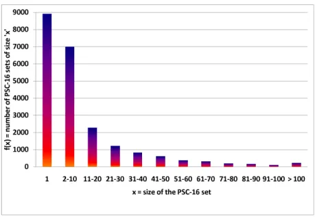
13 The histogram of the prefixes sharing the first 16 bits. . . 45
14 The overflow of CHAP(1, m) vs. linear probing(1, m) for table rrc07. . . 46
15 The (a) Average overflow, and (b) AMAT for CHAP(3,3) vs. RH(6) for fifteen forwarding tables for C1: {L = 180 , N = 2048} . . . 47
16 The (a) Average overflow, and (b) AMAT of RH(5) vs. GH(5) vs. PH(5) for fifteen forwarding tables for C1: {180×2048}. . . 48
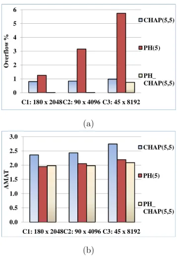
17 The (a) Average overflow, and (b) Average AMAT of CHAP(5,5) vs. PH(5) vs. PH CHAP(5,5) for three configurations. . . 49
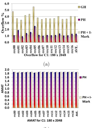
18 The (a) Average overflow, and (b) AMAT of GH vs. PH vs. PH+I-Mark for
fifteen forwarding tables for C1: {180×2048}. . . 50
19 The CACTI results of CA-RAM vs. TCAM, where both has sizes of 2.5MB. . 52
20 The CA-RAM detailed architecture for the packet classification application. . 56
21 The range matching circuit for the CA-RAM PC application. . . 57
22 The exact matching circuit for the CA-RAM PC application. . . 58
23 Applying PH on packet classification application. . . 59
24 The average tuple space representation of the 11 PC databases given in Table 3. 62
25 An example of the TSS representation ofACL530K db of Table 3.. . . 65
26 The two CA-RAM architecture: an overview. . . 67
27 The two CA-RAM architecture: the main CA-RAM row element format, the
results vector format and the auxiliary CA-RAM row format. . . 68
28 The auxiliary CA-RAM detailed architecture and its row format. . . 69
29 The (a) Average overflow of GH(6) vs. PH(6) + I-Mark, and (b) AMAT &
WMAT of PH(6) + I-Mark for the PC databases given in Table 3 for C1 :
{60×1K}. . . 73
30 The (a) Average overflow for GH(6) vs. PH(6) + I-Mark, and (b) Average
AMAT of PH(6) + I-Mark for the average PC databases in Table 3 for six
hardware configurations. . . 74
31 The Average Overflow of PH(6), PH(8) and PH(C) for the PC databases given
in Table 3 for six hardware configurations.. . . 75
32 The Average AMAT of PH(6), PH(8) and PH(C) for the PC databases given
in Table 3 for six hardware configurations.. . . 76
33 The average WMAT of regular PH(6), average PH(8) and custom cuts PH(C)
for the PC databases given in Table 3. . . 76
34 The regular single CA-RAM architecture vs. the equivalent two CA-RAM
architecture, whereL=L1+L2. . . 77
35 The overflow of the two CA-RAMs vs. the single CA-RAM architectures for
36 The AMAT of the two CA-RAMs vs. the single CA-RAM architectures for
The PC databases given In Table 3 for two hardware configurations. . . 78
37 The average overflow of single CA-RAM vs. two CA-RAM architectures for nine hardware configurations. . . 79
38 The average AMAT of single CA-RAM vs. two CA-RAM architectures for nine hardware configurations. . . 79
39 The overview of a DPI engine architecture. . . 83
40 An example of a SNORT [23] rule. . . 84
41 The SNORT statistics: percentage of patterns vs. the pattern lengths. . . 85
42 The modified CA-RAM variable-sized length patterns matching architecture. 86 43 The input shifting circuit2 of Figure 42. . . 88
44 The modified CHAP scheme example, where H = 4 andP = 2. . . 90
45 The overflow and the AMAT (using I-Mark) of SNORT for C1 :{512×256}, H = 3,4,5,6 and Lmax = 8,16,36. . . 94
46 The dynamic PH with I-Mark: (a) Overflow, and (b) AMAT of SNORT for H = 4 andLmax = 8,16,36. . . 96
47 The Dynamic PH + I-Mark: (a) Overflow, and (b) AMAT (I-Mark) of SNORT for H= 5 and Lmax = 8,16,36. . . 97
48 The dynamic PH + modified CHAP(H, P) and I-Mark: (a) Overflow, and (b) AMAT (I-Mark) of SNORT forH = 5, P = 4 andLmax = 8,16,36. . . 98
49 The TCAM vs. CA-RAM in terms of: (a) Total time delay, (b) Maximum operating frequency, (c) Total dynamic power and (d) Total area. . . 100
LIST OF ALGORITHMS
1 The CHAP(H,H) Setup Algorithm.. . . 24
2 The CHAP Search Algorithm. . . 26
3 The CHAP Insert Update Algorithm. . . 29
4 The PH Setup Algorithm. . . 34
LIST OF EQUATIONS 3.1 Equation (3.1). . . 9 3.2 Equation (3.2). . . 9 3.3 Equation (3.3). . . 9 4.1 Equation (4.1). . . 21 4.2 Equation (4.2). . . 22 7.1 Equation (7.1). . . 98 7.2 Equation (7.2). . . 99 7.3 Equation (7.3). . . 99 9.1 Equation (9.1). . . 105
PREFACE
Acknowledgments
To both Dr. Rami Melhem and Dr. Sangyeun Cho, my advisors and also to Dina, Mira and Matthew, my little beautiful family.
1.0 INTRODUCTION
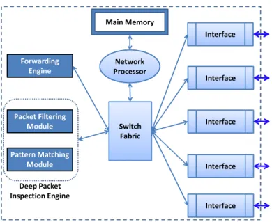
A router, as shown in Figure 1, consists of multiple interface cards (egress and ingress), a switch fabric, a CPU or a network processor (NP) that is attached to a memory module (this could be a hierarchy of caches [11]), a forwarding engine, and either a deep packet inspection (DPI) engine (in case the router has a firewall capabilities) or a QoS engine for traffic shaping. Both the DPI engine and the QoS unit contain a packet filtering (classification) unit.
The router’s main function is to receive data packets and forward them to their correct destinations. It inspects the packet’s IP (internet protocol) headers and extracts the des-tination of this packet via looking it up in its forwarding table. High-speed routers have become very desirable as they facilitate the rapid transfer of packets. In addition to their basic packet forwarding (PF) functionality, most modern routers also inspect the remaining packet (e.g., TCP) headers to determine what access rights or what service (bandwidth) this packet might have. This is called packet classification (PC) functionality.
High-speed Internet routers and firewalls require wire speed packet-processing, while the sizes of their DPI and PC rule databases and PF tables are increasing at a high rate [31, 53,
54]. In addition, the advancement of optical networks keeps pushing the link rates, which are already beyond 40 Gbps [43, 54]. In this thesis, we focus on the three main components of the high-speed Internet router: the packet forwarding engine, the packet filtering engine and the deep packet inspection engine. We note that these three engines are similar in the sense that they all rely on search-intensive operations.
In packet forwarding (PF), the destination address of every incoming packet is matched against a forwarding table to determine the packet’s next hop on the way to its final des-tination. An entry in the forwarding table, or an IP prefix, is a binary string of a certain length followed by wildcard (don’t care) bits and an associated port number. The actual
Switch Fabric Forwarding Engine Pattern Matching Module Packet Filtering Module Deep Packet Inspection Engine Interface Network Processor Main Memory Interface Interface Interface Interface
Figure 1: A generic router architecture with deep packet inspection capability.
matching requires finding the “Longest Prefix Matching” (LPM) as instructed in the CIDR protocol [39].
In packet classification (PC), a packet header is matched against a database of rules–or filters–to obtain the best matching rule. A priority tag is appended to each rule, and the packet classifier must return the rule with the highest priority as the best-matching rule in case of multiple matches. Each filter consists of multiple field values. The number of fields per rule and the number of bits associated with a field are variable and depend on the application. Typically, filtering is applied to the following fields (tuples [47]): IP source address, IP destination address, source port, destination port and protocol identifier. Rules are associated with either an “action” (e.g., in case of firewall) or a “flow ID” (e.g., in case of QoS).
In deep packet inspection (DPI), the firewall examines the packet’s payload for traces of either network attacks, such as network intrusion detection system (NIDS) or malware signatures, such as virus scanning systems [33]. The main components of a DPI engine are the pattern-matching (PM) unit [59], and the packet filtering unit [33]. The packet pattern-matching problem is defined as follows: given a set of k patterns {P1, P2,· · ·, Pk}, k ≥ 1,
and a packet of length n, the goal is to find all the matching patterns in the packet. Note that each pattern (string) has its own length. If we match one or more of these substrings, we have a “partial” match and the pattern-matching unit should return the longest matched substring to the software layer of the firewall for further investigation. In addition to DPI, content filtering, instant-messenger management, and peer-to-peer identification applications all use pattern (string) matching for inspection [33]. Throughout this thesis we will refer to any of a prefix, a PC rule or a DPI pattern as a “key.”
The two main streams of packet-processing research are: algorithmic and architectural. Many researchers have devised algorithmic solutions that provide space and time complexity bounds for difficulties arising in packet-processing [19,18,26,47,15]. Some of these solutions are feasible for hardware implementations [51, 33, 15]. In general, the algorithm-based solutions have lower throughput than their hardware counterparts. This motivated the introduction of architectural solutions that mostly rely on the Ternary Content Addressable Memory (TCAM) technology [28,46]. A TCAM is a fully associative memory that can store binary values, 0s and 1s as well as wildcard (don’t care) bits. TCAMs have been the de
facto standard for packet-processing in industry [31, 53, 33]. However, TCAM comes with
significant inefficiencies: high power consumption, low bit density, poor scalability to long input keys, and higher cost per bit compared to other memories.
In addition to these two research streams, the industry recently started to adopt em-bedded DRAM [58] (eDRAM) technology. eDRAM is a capacitor-based dynamic RAM that is integrated on the same die as the main ASIC (application specific integration circuit) or processor, which allows the network processor chip to have more memory. This direc-tion is pioneered by “Huawei” Technologies [6] who call their technology Smart Memory, “NetLogic” and “Cavium.”
Architectural solutions based on hashing have also been proposed [16, 29, 44, 47, 15]. Hash tables come in two flavors: closed addressing hash (or chaining) and open addressing hash. A hash table in closed addressing hash has a fixed height (number of buckets), and each bucket is an infinite size-linked list. In open addressing, a hash table has both a fixed height and a fixed bucket width. Overflow in open addressing hash is handled through probing [13], as described in Section 3.1. We define the overflow as being the percentage of keys that did
not fit into the main hash table to the total number of keys available for storage. In this thesis, we assume open addressing hash and our goal is to fit the packet-processing database in a single fixed-size hash table with minimal overflow, high space utilization and low average memory access time. The power consumption issue will be addressed almost automatically by storing this hash table in an efficient SRAM or DRAM memory array.
The remainder of this thesis is organized as follows:
• In Section 3, we give a brief background on: general open addressing hashing, hash-ing with the presence of wildcards, and finally we illustrate our set-associative memory architecture.
• In addition, in Section4, we describe our hashing schemes, which are used later as tools in our packet-processing engines.
• in Sections 5, 6, and 7 we describe our solutions and experimental results to each of the three packet-processing applications.
2.0 THESIS OUTLINE, MOTIVATION AND CONTRIBUTIONS
In this section, we describe the ‘big picture’ of our thesis. We mentioned that the subjects of this thesis are the router’s search-intense packet-processing units; namely, the forwarding engine, the packet filtering engine and the deep packet inspection engine. Since the target of today’s and future Internet routers and firewalls is to keep up with both IPv6 and new ultra high link rates, we need to think about packet-processing units designs that have high throughput and have low power consumption all at the same time. We choose a design that is based on a set-associative memory hardware realization of hash tables, as it provides a general homogeneous platform for all the three applications. The actual architecture we are using is called CA-RAM (Content Addressable-Random Access Memory) and is described in some detail in section3.4.
In general, The CA-RAM provides a reliable RAM architecture for search intensive applications [12]. It allows for concurrent searching through multiple keys. In addition, it is based on regular RAM technology rather than the expensive TCAM technology. Finally, the CA-RAM is better than the classical hardware TCAM-based solution in its ability to support different types of matching. For example, the packet classification application requires three different types of matching: prefix matching, exact matching and range matching. While the TCAM naturally supports both exact and prefix matchings, it requires the addition of special complex hardware to deal with the range matching [46]. On the other hand, CA-RAM supports all aforementioned types of matching, due to its unique feature of separating the storage capability from the matching logic.
We believe that such architecture is capable of answering the wire speed and the power consumption issues much better than other hardware and software solutions. The high throughput requirement is boosted by using pipelining. For CA-RAM to work efficiently,
it needs good hashing schemes to fully utilize its capabilities. For example, in the PC and PF applications, the keys that are being mapped into the hash table have low entropy and tend to collide. Also, in the DPI application, some strings are substrings of other strings in the DPI rule database. Thus CA-RAM needs new, efficient, collision-resolving schemes that are more efficient than classical linear and quadratic probings. These new hashing schemes should allow for high space utilization of the CA-RAM. I talk more about probing in the next section, Section3.1.
At the same time, CA-RAM also needs to maintain a high throughput, which is achieved by lowering the memory access time and using pipelining. Thus our proposed hashing schemes should lower the memory access time for the CA-RAM while resolving the collision problem, which are two contradictory goals. In addition, in packet-processing applications, the search engine, in this case the CA-RAM, has to report first the best matching key in the database. In case of PF, the CA-RAM has to return the longest matching prefix, while in the DPI, the CA-RAM has to return the longest matching pattern. Thus, our hashing schemes have to support this property. Finally, since packet-processing applications require dealing with wildcards, my hashing schemes have to deal with this issue as well.
In this thesis, I am proposing three hash-based schemes (techniques) that enable the use of the CA-RAM for the three packet-processing applications. These are (in order of presentation): content-probing pointers, progressive hashing and independent marking (I-mark). These techniques are fully developed for two applications, namely PF and P,C and are extended to the DPI application with some additional hardware customization. These schemes are defined as our building blocks in Section 4. In addition, each scheme will be optimized for each application, as described in Sections 5,6 and 7.
My first scheme, the content-hash probing or CHAP, is–as its name indicates–a probing technique that relies on the actual stored data in the hash table to probe for overflow keys. This is in contrast to the classical systematic probing techniques (e.g., linear and quadratic) that are known in the literature, which do not take into account the stored data and its distribution. The third way to handle probing in open address hashing is double hashing. My second hashing scheme, progressive hashing, extends double hashing, which is a known technique for open address hashing (see Section3.1), by first splitting the keys into different
groups. We then assign to each group a unique hash function to reduce the collision prob-ability. This is different than double, or multiple, hashing where all keys can use all hash functions that are used by the system. Finally, I propose my third technique, the I-mark, to take advantage of the fact that some keys can be parts of other keys, like in DPI where some short strings are substrings of other longer strings. In this technique, I use the fact that some keys are truly independent or unique (i.e., have no other keys shorter or longer that are parts of these keys, nor are these keys part of other keys) to store the keys efficiently inside the CA-RAM. This is so we can insert those unique keys before or after other keys to lower the chance of collisions.
As I am going to show in the rest of this thesis, the CA-RAM, along with my pro-posed hashing schemes, outperforms the TCAM. I prove this by conducting a battery of experiments and simulations to compare both CA-RAM and TCAM in terms of throughput (speed), power consumption and space area. For example, my modified CA-RAM is esti-mated to be capable of processing up to 320 Gbps for PF application, and is 160 Gbps for the PC application, while our CA-RAM speed runs at a clock frequency of 540MHz. While achieving such high rates of processing in these three application, the CA-RAM power con-sumption is less than its equivalent size TCAM by 77% for the PF application and 71% for the DPI application. Moreover, we consider that the CA-RAM is much more scalable than the TCAM due to the fact that it separates the storage from the matching part.
3.0 BACKGROUND
In this chapter, in Section 3.1, I describe open addressing hash from the theoretical point of view, while in Section 3.2, I address the issue of using single versus multiple hash tables. This issue stems from the fact that some of the proposed solutions for packet-processing rely on multiple hash tables. In Section 3.3, I talk about hashing keys with wildcards and how they can cause collisions. In Section 3.4, I describe in some detail the CA-RAM general architecture and it advantages over the TCAM. At the end of this chapter, in Section 3.5, I summarize some of the related work.
3.1 GENERAL OPEN ADDRESSING HASH
Searchable data items, or records, contain two fields: key and data. Given a search key, k, the goal of searching is to find a record associated with k in the database. Hash schemes achieve fast searching by providing a simple arithmetic function h(·) (hash function) on k, so that the location of the associated record is directly determined. The memory containing the database can be viewed as a two-dimensional memory array of N rows with L records per row.
It is possible that two (or more) distinct keys ki 6=kj hash to the same value: h(ki) =
h(kj). Such an occurrence is called “collision.” A worst-case (pathological) situation that restricts the effectiveness of hashing is when all the keys are mapped to the same row. There are two solutions to the collision problem in this case: 1) Make the row large enough to hold all the possible colliding prefixes at the cost of a large amount of wasted memory. 2) Control the row size and handle the overflow prefixes in a different way, such as “probing.”
When there are too many (≥ L) colliding records, some of those records must be placed elsewhere in the table by finding, or probing, an empty space in a bucket. For example in
linear probing, the probing sequence used to insert an element into a hash table is given as
follows:
h(k), h(k) +β0, h(k) +β1,· · · , h(k) +βm−1 (3.1)
where each βi is a constant, and m is the maximum number of probes. Linear probing is simple, but often suffers from what is called “primary key clustering” [13].
Another type of probing is called quadratic probing, where we use a quadratic equation to determine the next bucket to be probed. The quadratic probing sequence used to insert an element into a hash table is generated by the following equation:
h(k, i) = (h0(k) +c1×i+c2×i2)mod(N), i= 0,1,· · ·m−1 (3.2)
whereh0(·) is called the auxiliary hash function and bothc1 andc2 are constants. Quadratic
probing suffers from another type of clustering, called “secondary key clustering” [13]. Instead of probing, we can apply a second hash function to find an empty bucket, a procedure know asdouble hashing[13]. In general, the use ofH ≥2 hash functions is shown to be better in reducing the overflow than probing [2]. In this case (which we refer to as
multiple hashing) the probing sequence of inserting a key into the hash table is given as
follows:
h0(k), h1(k),· · · , hH−1(k) (3.3)
where H is the number of hash functions. To achieve high space utilization (or load factor, which is the ratio between the size of the database and the capacity of the actual RAM used to store it) we apply multiple hash functions on a single hash table, rather than using a separate table for each hash function [8].
3.2 USING SINGLE HASH TABLE VS. MULTIPLE HASH TABLES
Note that using a different hash table for each hash function in Equation3.3is a valid design option; however, using different hash tables leads to more overflow, Hence results in poor space utilization [14, 26, 54]. In what follows, we argue that using a single hash table is better than using multiple hash tables.
Consider the case where we have two identical hash tables, A and B, of size (N ×L), where N = number of rows and L = row width, and the case where we have an equivalent single hash table, C, of size (N ×2L). Assume that ‘a’ elements are mapped to row i of table A and ‘b’ elements are mapped to row i of table B, then ‘c’ = (a+b) elements are mapped to row, i, of table C. The overflow is calculated for tables A, B and C, respectively, as follows:
overf lowA=max{0,(a−L)}
overf lowB =max{0,(b−L)}
overf lowC =max{0,(c−2×L)}
It is straightforward to show that if (a > L and b > L) or (a < L and b < L), then:
overf lowC = (overf lowA + overf lowB). If one of ‘a’ or ‘b’ is larger than L and the other
is smaller thanL, then overf lowC <(overf lowA+overf lowB). Specifically, if (a =L+x) and (b = L −y) for some integers x, y > 0, then (overf lowA +overf lowB = x) while
(overf lowC = 0) or (x−y) when (y < x or y > x), respectively. Thus, having more than
one hash table results in larger overflow than having a single hash table.
To achieve high space utilization (load factor) we apply multiple hash functions on a single hash table. Specifically, a key is inserted in the hash table using any of the H hash functions in Equation 3.3. Given a database of M records and an N-bucket hash table, the average number of hash table accesses to find a record is heavily affected by the choice of
h(·), L (the number of slots per bucket), and α, or theload factor, defined as M/(N ×L). With a smaller α, the average number of hash table accesses can be made smaller, however at the expense of more unused memory space [3].
3.3 HASHING WITH WILDCARDS
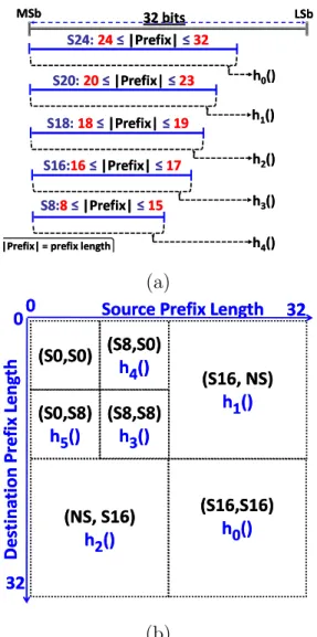
Applying hash functions in packet-processing applications is very challenging due to the fact that wildcards, or don’t care bits, are heavily present in the packet-processing en-gine’s database. Hashing with wildcards requires one of two solutions: restricted hashing or grouped hashing [20]. In restricted hashing RH, the hash functions are restricted to using only the non-wildcard bits of the keys. We use RH only for PF application. In grouped hashing, GH, keys are grouped based on their lengths, then different hash functions are applied to each group. By length we mean the part of the key that does not contain any don’t care bits, which we call “specific bits.” For example, the 32-bit IPv4 address can be split into 5 groups as follows:
- GroupS24, containing prefixes with at least 24 specific bits. - GroupS20, containing prefixes of length between 20 and 23 bits.
- GroupS18, containing prefixes of length 18 and 19 bits. - GroupS16, containing prefixes of length 16 and 17 bits. - GroupS8, containing prefixes of length between 8 and 15 bits.
Then, each group is associated with a different single hash function as shown in Fig-ure 2(a). We represent the 32-bit address space with a bold line, whereM Sb andLSb stand for most significant bit and least significant bit, respectively.
Grouped hashing can also be applied to PC using the tuple space concept. For example, a coarse-grained tuple space [45] (we describe this scheme in Section 3.5), where a key is of the form (source address prefix, destination address prefix), can divide the PC hashing space (or keys to be hashed) into 7 groups, as shown in Figure 2(b). The filters are split into 4 groups based on the source and the destination prefix lengths: (S16, S16), (S16, N S),
(N S, S16) and (N S, N S), where “S16” means that the prefix has 16 or more specific bits,
while the “N S” stands for Non-Specific, i.e., the prefix is less than 16 bits. The (N S, N S) group is split once more into 4 groups: (S8, S8), (S8, S0), (S0, S8) and (S0, S0), where “S0” includes all prefixes that are less than 8 bits long.
32 bits 32 bits S24: S24: 2424≤ ≤ |Prefix| |Prefix| ≤ ≤ 3232 MSb MSb LSbLSb hh00()() hh11()() hh22()() hh33()() hh44()() S20: S20: 2020≤ ≤ |Prefix| |Prefix| ≤ ≤ 2323 S18: S18: 1818≤ ≤ |Prefix| |Prefix| ≤ ≤ 1919 S16: S16:1616≤ ≤ |Prefix| |Prefix| ≤ ≤ 1717 S8: S8:88≤ ≤ |Prefix| |Prefix| ≤ ≤ 1515
|Prefix| = prefix length |Prefix| = prefix length
(a) (S16,S16) (S16,S16) hh00()() (NS, S16) (NS, S16) hh22()() (S16, NS) (S16, NS) hh11()() (S0,S8) (S0,S8) hh55()() (S0,S0) (S0,S0) 00 3232 00 32 32 Source
Source Prefix Prefix LengthLength
De st in at io n De st in at io n Pr ef ix Pr ef ix Le ng th Le ng th (S8,S0) (S8,S0) hh44()() (S8,S8) (S8,S8) hh33()() (b)
Figure 2: Splitting the hashing space into groups for (a) PF application, and (b) PC Appli-cation.
3.4 THE CONTENT ADDRESSABLE-RANDOM ACCESS MEMORY
(CA-RAM) ARCHITECTURE
We use the CA-RAM as a representative of a number of set-associative memory architectures proposed for packet-processing [12, 26, 60]. CA-RAM is a specialized, yet generic memory structure that is proposed to accelerate search operations. The basic idea of CA-RAM is simple; it implements the well-known hashing technique in hardware. The key features of
the CA-RAM are that it separates the matching logic from the storage, allowing for greater space saving over regular CAMs. At the same time keeping the matching logic near the memory bulk, allowing for lower I/O bandwidth and lower processing latency [12].
CA-RAM uses high-density memory (i.e., SRAM, DRAM or eDRAM [58]) and a number of small match logic blocks to provide parallel search capability. Records are pre-classified and stored in memory so that given a search key, access can be made accurately on the memory row having the target record. Each match logic block then extracts a record key from the fetched memory row, usually holding multiple candidate keys, and determines if the record key under consideration is matched with the given search key.
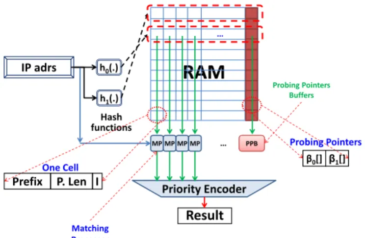
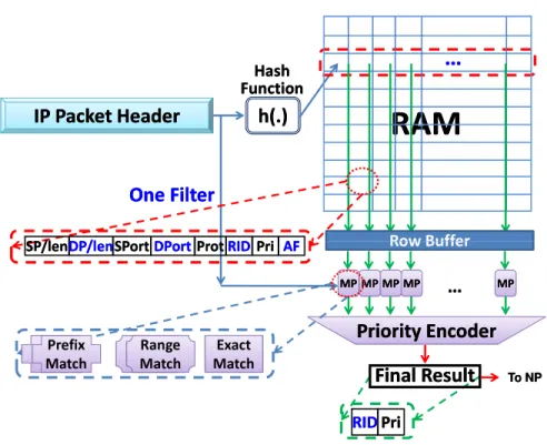
CA-RAM provides a row-wise search capability comparable to TCAM. More importantly, the bit-density of CA-RAM is much higher than that of TCAM, up to nearly five times higher if DRAM is used in the CA-RAM implementation [12]. A CA-RAM takes a search key as an input, and outputs the result of a lookup. Its main components are: an index generator, a memory array (SRAM or DRAM), and match processors, as shown in Figure 3. The task of the index generator is to create an index from an input key. The actual function of the index generator depends highly on the target application. Depending on the application requirements, a small degree of programmability in index generation can be implemented using a set of simple shift functions and multiplexers.
A row may be divided into entries of the form shown at the left corner of Figure3, where a CA-RAM entry (cell) stores a key, and its corresponding data. Alternatively, two bits can be used to store a ternary digit to represent 0, 1 and don’t care, rather than binary (as in TCAM arrays, except that the comparison hardware in this case is shared among all the rows in the memory array). Optionally, each row can be augmented with an auxiliary field to provide information on the status of the associated bucket (e.g., how many keys are stored in this row). We use the auxiliary field in our hashing schemes as we will see later.
RAM
Index Generator IG Key An element is mapped to this rowMP MP MP MP MP Matching Processors Priority Encoder Result One Cell Key Data Parallel Matching
Figure 3: The CA-RAM as an example of set-associative memory architectures.
Once the index is generated from the input key, the memory array is accessed andL can-didate keys are fetched simultaneously. The match processors then compare the cancan-didate keys with the search key in parallel, resulting in constant-time matching. Each match proces-sor performs comparison quickly using an appropriate hardware comparator. For example, if we are comparing PC range field, then the matching processor is simply a range comparator, while when we are comparing either PF prefix field or a DPI string, the matching processor consists of an exact matching comparator.
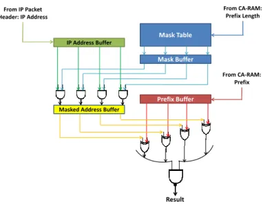
Figure4shows a simple key matching circuit for a generic RAM. We assume that CA-RAM is being queried for a certain key (stored key) using another external key. Throughout my thesis, the external key will be extracted from some IP packet (header or payload). After the key is fetched from the storage section of the CA-RAM (i.e., RAM), it is stored in a buffer that we call a “key buffer.” This key is going to be compared against the key part of the incoming element, which is stored in another buffer, “I/O buffer.” For simplicity, we assume that this is exact matching where we use just simple XOR gates to make sure that both the stored key and the external key are identical.
External Key Buffer From CA-RAM: Key From I/O: Key Key Buffer Result to Priority Encoder
Figure 4: A simple key matching circuit for a generic CA-RAM.
A large area saving in CA-RAM comes from decoupling memory cells and match logic. Unlike conventional CAM, where each individual row in the memory array is coupled with its own match logic, CA-RAM completely separates the dense memory array from the common match logic (i.e., match processors). Since the match processors are simple and lightweight, the overall area cost of CA-RAM will be close to that of the memory array used. At the same time, by performing a number of candidate key matching operations in parallel, low-latency, constant-time search performance is achieved.
CA-RAM was compared against TCAM in terms of performance, power and area (cost). The result obtained in [12] shows that CA-RAM is over 26 times more power-efficient than the 16T SRAM-based TCAM [30], and over 7 times more than the 6T dynamic TCAM [34]. The CA-RAM cell size is over 12 times smaller than a 16T SRAM-based TCAM cell, and 4.8 times smaller than a state-of-the-art 6T dynamic TCAM cell.
Overall, CA-RAM is performance-competitive with TCAM, in terms of both search la-tency and bandwidth. The detailed area and power issues are addressed in [12].
3.5 RELATED WORK
In this section, we review hash-based solutions that were proposed for each of the packet-processing applications. Most of the work that is done in hash-based packet-packet-processing uses closed addressing hash [7,29,44,8]. One of the few solutions that are based on open address hashing in the PF application is the IPStash [26, 27]. The IPStash architecture is similar to the CA-RAM architecture [12,26,27]. However, IPStash uses a special form of the grouped hashing scheme as it classifies the prefixes into only three groups according to their lengths, and uses only 12 bits for hash table indexing. In addition, IPStash uses controlled prefix expansion (CPE) [48] to expand prefixes of lengths between 8 and 15 bits to 16 bits, and then choose any 12 bits to index the hash table [27]. In our work [21], we compared our CA-RAM-based schemes against IPStash and showed that our schemes are superior.
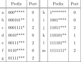
Prefix Port Prefix Port a 000***** 0 h 1******* 0 b 000101** 1 i 1001**** 0 c 0001111* 2 j 11011*** 2 d 0010**** 0 k 110101** 1 e 00111*** 2 l 111101** 1 f 0110**** 0 m 1111111* 2 g 01111*** 2
Table 1: An example of an 8-bit address space forwarding table.
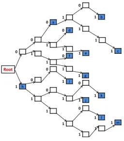
The most well-known PF algorithm-based solutions use the binary trie data structures. According to [42], a trie is: “a tree-like data structure allowing the organization of prefixes on a digital basis by using the bits of prefixes to direct the branching.” Table 1 shows an example of an IP forwarding table assuming 8-bit addressing. Figure 5 is the equivalent binary trie of the IP forwarding table shown in Table1, wherea, b,· · · , mare symbols given to the prefixes for easy identification. The main advantages of trie-based solutions are that they provide simple time and space bounds. However, with the 128-bit IPv6 prefixes, both trie height and enumeration become an issue when the prefixes are stored inside the nodes.
Root 0 1 h 0 1 0 a 1 0 1 b 1 1 c 1 0 d 1 1 1 0 f 1 0 1 1 j 0 1 k 1 1 0 1 l 1 1 0 0 1 i 1 1 m 1 e 1 g
Figure 5: The binary trie representation of the forwarding table given in Table 1.
For the PC application, the authors in [47] introduce a special hash-based scheme called Tuple Space Search (TSS). In TSS, the five PC fields are represented by a “tuple,” which is simply a group of integers substituting the actual fields. A prefix is represented by an integer that equals the number of its defined bits; each range is converted to two integers using range encoding, and each protocol is represented by an integer.
The original TSS scheme suffers from having high worst-case search time of O(W2),
where W is the prefix length in bits. The authors then introduced an optimization called “markers and computations.” Each tuple has two pointers to two filters; a marker (filer) and a precomputation filter. During a search for the best matching filter for any incoming packet, we probe to a tuple Ti, where we have two choices:
• The packet we have matches one of the filters that belong to Ti, in which case we need to find a more specific filter.
• The packet does not match any filter, in which case we need to find a less specific filter.
A marker filter is a pointer to the less specific filter than the current matching filter inTi, while a precomputation filter is a pointer to the more specific filter. Note that the specificity of a certain filter in the 2D TSS is determined by the length of both prefixes of this filter.
In [32], the authors introduced an optimization to the TSS scheme by introducing a binary search scheme on 2D tuples space. However, this optimization [32] did not address
the practical issues of the TSS such as: how to handle the multiple hash tables, and how to select the hash functions. The work by Song et al. [45] is the first to show how a practical TSS system functions by splitting the 2D TSS into coarse clusters, and then assigning one hash table to each cluster. The work in [29] enhances [45] by using other kinds of summaries instead of the Bloom filter-based [7]. A Bloom filters (BF) are simple array of bits used for representing a set to support fast approximate membership queries [7]. The main disadvantage of BFs is that they make false positive membership queries.
(a) (b)
Figure 6: The (a) Sliding window example, and (b) Its jumping window equivalent where
w=m= 4.
A DPI engine consists of two units: a PC engine and a pattern-matching engine [33]. Some of the DPI patterns are “simple” patterns, meaning they are concatenations of single-byte ASCII code characters (in which some wildcard single-bytes could appear in place) while there other patterns are called “composite” patterns. An example of the composite patterns would be what is known as “correlated” patterns, where subpatterns appear in specific locations inside the packet. Throughout our work, we assume only simple patterns and subpatterns. To process a composite pattern, the PM engine detects all the simple subpatterns that make that composite pattern and sends them to the network processor for further investigation.
but suffer great performance deficiency for large ones [33]. The TCAM width ‘w’ is an im-portant factor in the design of the pattern-matching unit. In [59], the authors describe a byte-by-byte scanning TCAM solution, which is referred to as a “sliding window” scheme [49]. In a sliding window scheme, a window of ‘w’ characters of each packet is compared to the content of the TCAM for a match. The problem with this approach is that the scanning speed is low, since each time a new character is being added to the window, another is being dropped, as depicted in Figure 6(a).
The authors in [49] propose an extension to the sliding window that is called “jumping window,” where at every clock cycle, a window of ‘m’ characters is jumped and a new window is inspected, as we can see in Figure 6(b). The throughput in this case is claimed to be multiples of that of the sliding window, however at the cost of replicating the same patterns m−1 times, as can be seen in Figure 6(b). In addition to TCAM solutions, a few closed addressing hash-based solutions are proposed [15].
In addition to these two research streams, there are also the automaton-based ap-proaches [33, 5, 4]. However, these approaches have an inherent complexity that limits the total number of Regular Expressions (or complex patterns) that can be detected using a single chip [4]. There has been a lot of progress in this area through either using the DFA (Deterministic Finite Automaton) or Non-Deterministic Finite Automaton (NFA) [10].
4.0 OUR DEVELOPED HASHING SCHEMES AND TOOLS
As we mentioned earlier in Section2, classical hash collision resolution schemes are inefficient for our packet-processing application while using the CA-RAM architecture. On one hand, the keys tend to have more collisions than the typical hashing of keys that are assumed to be uniformly distributed, while on the other hand, these schemes do not perform well with the CA-RAM architecture. For example, if we resolve hash collisions with linear probing, we might end up searching the entire CA-RAM for a certain key, which is not acceptable.
In this section we describe our proposed hash-based schemes that best suit both the three packet-processing applications and our main hardware architecture, CA-RAM. All our schemes are based on open addressing hash methodology; however, they could also be applied to the closed addressing hash methodology. These are all general schemes that are meant to work for the three applications. We introduce more specific optimizations in Chapters 5, 6
and 7 that exploit particular features of each application.
In Section 4.1, we describe our first hashing scheme, “Content-based HAsh Probing,” or CHAP. CHAP is an extension to the hash probing techniques introduced in Section 3.1. In Section 4.2, we discuss our “Progressive Hashing” scheme, which is an extension to the grouped hashing introduced in Section 3.1.
Finally, in Section4.3, we describe our “I-Mark” scheme. The I-Mark is a general scheme to mark those keys that are unique so that if we find one of them during a matching process, then we can stop looking for more matches. This helps in reducing the average memory access time (AMAT) and the overflow at the same time.
4.1 CONTENT-BASED HASH PROBING (CHAP)
As we mentioned in the last section, a CA-RAM row stores the elements of a bucket and is accessed in one memory cycle. Because the architecture is very flexible, we may keep some bits at the end of each row for auxiliary data; this allows for more efficient probing schemes with multiple hash functions. In this section, we first present the basic content-based hash probing scheme, CHAP(1,m), which is a natural evolution of the linear probing scheme described by Equation (3.1). We then extend this scheme to H hash functions, which we call CHAP(H,m).
In open addressing hash, some rows may incur overflow, while others have unoccupied space. While linear probing uses predetermined offsets to solve that problem, as specified by Equation (3.1), CHAP uses the same probing sequence, but with the constantsβ0, β1,· · · , βm determined dynamically for each value of h(k), depending on the distribution of the data stored in a particular hash table. Specifically, the probing sequence to insert a key “k” is:
h(k), β0[h(k)], β1[h(k)],· · · , βm−1[h(k)] (4.1)
This means that for each row, we associate a group of m pointers to be used if overflow occurs to point to other rows that have empty spaces. We call these pointers “probing pointers,” and the overall scheme is called CHAP(1,m)since it has only one hash function and m probing pointers per row.
Figure 7 shows the basic idea of CHAP whenm = 2. To match the overflow excess keys to specific rows, we need to collect all the overflow elements across all the rows. We achieve this by counting the excess elements per row, and finding for each row i two rows in which these overflow elements can fit. These two rows’ indices are recorded in β0[i] and β1[i].
Assume that we are searching for a keyk. If the hash function points to rowi=h(k) and it turns out that the input key k is not in this row, we check to see if the probing pointers at row iare defined or not. If defined, this means that there are other elements that belong to row i, but that reside in either rowβ0[i] or in rowβ1[i] and these elements might contain
k. Consequently, rows β0[i] and β1[i] are accessed in subsequent memory cycles to find the
Probing Pointers All elements at this row
are matched in parallel
h(.) Packet Packet To the Matching Processors … β ββ β1 β β β β0 …
Figure 7: The CHAP basic concept.
The content-based probing can also be applied to the multiple hashing scheme. Specifi-cally, we refer to CHAP with H hash functions and m probing pointers by CHAP(H,m). For example, in CHAP(H,H) we haveH hash functions and m=H probing pointers. In this case, the probing sequence for inserting a key, k, can be defined by:
h0(k), h1(k),· · · , hH−1(k), β0[h0(k)], β1[h1(k)],· · · , βm−1[hH−1(k)] (4.2) Probing Pointers Multiple hash functions h0(.) Packet To the Matching Processors … β β β β1[h1()] β β β β0[h0()] h1(.) … h2(.) β β β β2[h2()]
Figure 8: The CHAP(3,3).
In essence, we dedicate to each hash function a pointer per row. An example is shown in Figure 8for a three hash functions CHAP scheme, or CHAP(3,3), where a key is mapped
to three different buckets. In the example, this key will have six different buckets to which it can be allocated: h0(k), h1(k),h2(k), β0[h0(k)], β1[h1(k)] and β2[h2(k)] in the given order,
where βi[hi(·)] is the probing pointer of hash function hi(·).
There are different ways to organize CHAP(H,m) whenm6=H, depending on whether or not the probing pointers are shared among the hash functions in a given row. In the example described above for CHAP(H,H), we assume that one probing pointer is associated with each hash function. Another organization could share probing pointers among hash functions. Yet a third organization could assign multiple pointers for each hash function, which is the only possible organization for CHAP(1,m), when m >1. In Chapters 5 and 6, we limit our discussion to CHAP(1,m) and CHAP(H,H) with one pointer for each hash function and with the probing order given by Equations4.1 and 4.2 for the two organizations, respectively.
4.1.1 The CHAP Setup Algorithm
The main idea in this section is to prepare the keys and insert them into the CA-RAM hash table, which we call “setup phase.” Algorithm 1 lays out the setup phase of CHAP. Before we describe the actual algorithm, we discuss an important issue, which is to reduce the search time for the CHAP algorithm. To achieve this, we have to stop at the first matching key during search in the CHAPs search algorithm, Algorithm 2. This is done by storing the keys according to their specificity (priority) from the most to the least [19]. The priority (specificity) of a key depends on the key type. In PF application, the key priority is just the prefix length; the same goes for the strings (signatures 1) of the DPI application. However, there is a distinct priority value associated with each PC rule.
In Algorithm1,j = 0,· · ·, M−1 is used to index the keys, where M is the total number of keys in a packet-processing database. Our hash table has 2R = N rows, where R is the number of bits used to index the hash table. We usei as an index for hash functions andH
as the maximum number of hash functions. An array of counters,HC[ ] of sizeN, is used to count the number of elements that will be mapped to each row of the hash table. We define a two-dimensional array of countersOC[ ][ ] of size N×H to count the overflow elements for
1Throughout this thesis we will use both termssignatureandstringinterchangeably to present the same
each hash function per row. The maximum value of a single counter in this array is equal toλ, where λ≤L, andL is the number of keys stored per row. This bound comes from the fact that a hole, or an empty space in any row of the hash table, can never exceed L. The CHAP setup phase determines if the configuration parameters of the hash table are valid or not. In other words, do the parameters L, H, λ and N result in a mapping of the M keys into a single hash table with acceptable overflow or not?
Algorithm 1The CHAP(H,H) Setup Algorithm. 1: CHAP Setup(packet-processing Database)
2: Sort the keys according to specificity from highest to lowest 3: initialize the arrays HC[ ] and OC[ ][ ] to zeros
4: table overflow = number of keys that will not hashed to the CA-RAM
5: for(j = 0;j < M;j + +) {
6: inserted =f alse
7: for(i= 0;i < H;i++) {
8: ri =hi(kj) }
9: for (i= 0; i < H AND inserted == f alse; i++) {
10: if(HC[ri]< L),then {
11: HC[ri]++
12: inserted =true }
13: }
14: for (i= 0; i < H AND inserted == f alse;i++) {
15: if(OC[ri][i]< λ), then { 16: OC[ri][i]++ 17: inserted =true } 18: } 19: table overflow++ 20: }
Algorithm 1 calculates the number of keys to be assigned to each row. By “assigned,” we mean not only the keys that are hashed to this row, but also the overflow keys that are supposed to be in this row but that will reside in other rows to which this row’s probing
pointers point. It starts by sorting keys from highest priority to lowest priority, then initializ-ing the two arraysHC andOC to zeros, while the table overflow counter is initialized to the number of keys that are not going to be inserted in the hash table, because they are shorter than the minimum length the CA-RAM can handle (lines 1–2). Sorting the keys helps to stop at the first matching key, as will be proved in Section 4.1.2. The set of hash values
{r0,· · ·rH−1} for each key is calculated (lines 6–7). Then, the algorithm updates eitherHC
orOC as follows: if there is a spot for the current key in HC, then the algorithm increments
HC (lines 8–11); if not, it increments the corresponding OC counter (lines 12–15). In any case, the algorithm moves on to the next key.
When Algorithm1exits, table overflow will include the number of keys that could not fit in either HC orOC (lines 16–17). If this number is not acceptable, then the algorithm can be repeated with more hash functions, that is with a new H0 =H + 1. In that setting, the acceptability of the overflow depends on the capacity of the overflow buffer2. The progressive hashing scheme discussed in Section4.2may be applied in conjunction with CHAP to further reduce the overflow.
After completing the setup algorithm, we run a simple best-fit algorithm over the two arrays OC and HC, where we assign each overflow counter an address to a row that has a suitable hole that can accommodate the overflow keys. These addresses are what we call “probing pointers,” and they are one per row per hash function. Finally, we populate the hash table by simply mapping the keys into their rows using the same hash functions that we used in Algorithm 1. Once we have overflow for a certain row and a certain hash function, we use the probing pointer associated with this pair to put the key into a different row. Note that we are using a small TCAM chip to store the overflow, i.e., “overflow buffer,” where we us it to store prefixes for PF application, rules for PC application and filters for the DPI application. We search the overflow buffer after searching the main CA-RAM, which is covered in the next section, Section 4.1.2.
2Throughout this thesis we use the term “overflow buffer” to represent a small embedded TCAM module
4.1.2 Search in CHAP
In this section I discuss how search for a certain key is done in a CHAP-based hash table. We call our main hash table “H Table[ ][ ],” of size N×Lwhere N and Lare respectively the number of rows and the row capacity. Each element in H Table[ ][ ] consists of the actual key, H Table[ ][ ].key, and a couple of corresponding fields: an ID number, H Table[ ][ ].ID and the priority, H Table[ ][ ].pri. The key priority is used to determine the most specific key (MSK), while the key ID is a unique ID number that is reported back to the control plane software, which is used for incremental updates of the keys database.
As discussed in Section 3.4, a read operation fetches a full row (bucket) from the hash table into a buffer and uses a set of comparators to determine, in parallel, the most specific key in that bucket. A complete search might need to search more than one bucket. To measure the efficiency of the search in CHAP, we use the “Average Memory Access Time”, AMAT, which is the average number of rows accessed for successful search.
Algorithm 2The CHAP Search Algorithm. Search Hash Table(Key, K) {
1: for(i= 0 ; i < H ; i+ +) {
2: ri =hi(K)
3: ri+H =βi[hi(K)] }
4: for(i= 0 ; i <2H ; i+ +) {
5: if(K matches H Table[ri][j].key),
then { /* done in parallel for all values of j */ 6: returnH Table[ri][j].num }
7: }
8: search the overflow buffer}
The CHAP search algorithm, Algorithm 2, is straightforward. Given a key K, we cal-culate the row address ri(K) = hi(K) and ri+H =βi[hi(K)], where i = 0,· · · , H −1 (lines 1–3). For each row of the 2×H rows, we match the key against all the keys in this row in parallel, and if we hit at this row, we return the key ID number associated with the key (lines 4–6). If we do not find a match in these rows, we search the overflow buffer (line 8).
In Section 4.1.1, we discussed the importance of storing the keys according to their priorities to be able to stop at the first matching key during the CHAP search algorithm. In addition to sorting and inserting the keys according to their priority, we have to maintain what is called the “hash order” during both insertion and search phases. The hash order is merely the order of applying the hash functions in addition to the order of accessing the probing pointers. Theorem 1 proves that these two conditions are enough to find the MSK first.
Theorem 1. In CHAP, the first matching key is the MSK if:
1. The keys are inserted in order of most specific to least specific.
2. The search’s hash order, which includes both the order of accessing the probing pointers and the order of applying the hash functions, is the same as the insertion’s hash order.
Proof. In a restricted multiple hashing scheme, all the H hash functions are applied to
all keys. For example, in the PF application, assume that we have M keys to be hashed and that they are sorted according to their length, from the longest to the shortest. Also, assume that the hash order during the insertion is as follows: r0(km),· · · , r2H−1(km), where
ri(km) = hi(km) for i = 0,· · ·H − 1 and ri(km) = βi[hi(km)] for i = H,· · · ,2H −1. In addition, assume that there exists a packet K that matches two prefixeskX andkY and that
kX is longer than kY. This means that kX is mapped to the hash table before kY.
Without losing the generality, assume that rt(kX) = rt(kY) = rt. We can see that it is impossible for kY to find a space in row rt if kX could not find a space. This means that if
kX is stored in row ri(kX) =rX and ifkY is stored in row rj(kY) = rY, then i < j. Hence, while searching for a match forK as follows: r0(K), · · · r2H−1(K), we will match kX at row
rX before matching kY at row rY.
Note that if both prefixes kX and kY in Theorem 1 are mapped to the same row, the matching processors will determine the MSK in this case.
4.1.3 The Incremental Updates Under CHAP
An important issue in the packet-processing domain is the incremental updates of the databases. The number of keys included in a packet forwarding database grows with time [22, 54]. The updates consist of two basic operations, Insert/Update and Delete a key. In CHAP, the delete operation is straightforward. For any key deletion operation, we find the key first, then we delete it by storing all zeros and then decrement the row counter
HC, which is used to keep track of the rows’ populations. Deleting a key from any row does not require shifting, since the matching processors will ignore the deleted key spot as it will contain all zeros.
The basic idea of the insert/update operation, which is detailed in Algorithm 3, is to find the appropriate row that the new key should fit in. In this algorithm, Algorithm 3, we take into account that we report the most specific key. If we find out that the key already exists in our CA-RAM, the existing entry will be updated.
Algorithm3consists of two functions,CHAP Insert Update()andInsert in Rows(). The first function, CHAP Insert Update(), determines the appropriate rows to insert the new keyKn (lines 16–21). The second function is where the actual insertion is made, as it take a new key Kn, then it tries to insert it in a row from a range of rows starting from row index
a all the way to row index b.
In the first function, the row array ri, which has a size of 2×H, is used to store the computed values of the hash functions of the new key, Kn, and the corresponding probing pointers (lines 2–4). Note that ri is a global variable ,because it has to be accessed by the second function, Insert in Rows(). For each rowri we match Kn against all the keys in this row and extract both the most specific key,Kl, and the least specific key,Ks, that match Kn (lines 5–7). We record the rows indicesl ands that includeKl and Ks if such matchings are found. Depending on how specific Kn is related to both Kl and Ks, we try to insert Kn in one of the 2H rows. This is done through anif−else construct (lines 8–15). The first case is when neither Kl nor Ks are defined (i.e., no matching), thus we can insert Kn into any row (lines 8–9). The second case, which is route update [22], is when Kn is equal to either
Algorithm 3The CHAP Insert Update Algorithm. 0: define ri as an integer array of 2×H elements 1:CHAP Insert Update (New Key Kn){ 2:for(i= 0; i < H; i+ +) {
3: ri =hi(Kn)
4: ri+H =βi[hi(Kn)] }
5:By searching the rowsr0,· · ·r2H−1, find: {
6: Kl = most specific key matching Kn and l = index of row containing Kl 7: Ks = least specific key matching Kn and s = index of row containing Ks } 8:if(Kl is not definedAND Ks is not defined ), then {
9: return(Insert in Rows(Kn, 0 ,(2H−1))) } /* insert kn in any of rows r0,· · · , r2H−1 */
10:else if ((|Kn| == |Kl|) OR (|Kn| == |Ks|)), then { 11: ReplaceKl orKs with Kn /*an update operation*/ 12: return (true)}
13:else if(|Kn|>|Kl|),then { return(Insert in Rows(Kn, 0, l))}
14:else if(|Kn|<|Ks|),then {return(Insert in Rows(Kn, s, (2H−1))) } 15:else, return(Insert in Rows(Kn, l,s))
}
16:Insert in Rows (key Kn, a, b) {
/* insert Kn in any of the rows ra, ra+1· · · , rb */ 17:for(i=a; i <=b;i+ +) { 18: if(HC[ri]< L),then { 19: insert Kn in ri and HC[ri]++ 20: return (true)} } 21:return (f alse) }
if |Kn|3 is larger than |Kl|, then we try to insert Kn into one of the buckets {r0,· · · , rl} if there is a space (line 13). In the next case we check to see if |Kn|<|Ks| is true, then we try to insert Kn in a row among {rs,· · · , r2H−1} (line 14). Finally, if |Ks| <|Kn| <|Kl|, then we try to put Kn in any row between rl and rs (line 15).
In any case, the functions terminate successfully if we are able to insertKn. Otherwise, we try to either insert Kn into the overflow buffer, or use a backtracking scheme like “Cuckoo hashing” [35] to replace an existing key, say Ky, from the hash table by Kn, then try to recursively reinsert Ky back into the hash table [14].
The implementation of the incremental updates algorithm is done in the control plane (which contains a network processor to perform the necessary computations). We propose that the actual updates are issued as a special case during the idle time of the CA-RAM.
4.2 THE PROGRESSIVE HASHING SCHEME
We introduce our Progressive Hashing scheme (PH) as another effective mechanism for reduc-ing collisions (hence overflow) for keys with wildcards (don’t care bits) usreduc-ing open addressreduc-ing hash systems. As we mentioned in Section 3.3, using multiple hash functions is efficient in reducing collisions in general. In the same section, the two multiple hashing schemes for dealing with don’t care bits are described. In the restricted hashing scheme (see Figure9(a)) the hash functions h00(),· · · , h03() are applied to all the keys in the hashing space, hence all hash functions are restricted to the specific (not the don’t care) bits. On the other hand, in the grouped hashing (see Figure 9(b)) we split the hashing space into groups and a single hash function is associated with each group. In Figure 9(b), functions h0(), · · ·, h3() are
associated with groups 0, · · ·, 3 respectively.
Restricted Hashing Scheme
Group 0 Group 1 Group 2 Group 3 hh00`(), `(), hh11`(), `(), hh22`(), `(), hh33`()`()
Grouped Hashing Scheme
Group 0 Group 1 Group 2 Group 3 hh00()() hh11()() hh22()() hh33()() (a) (b)
Progressive Hashing Scheme
Group 0 Group 1 Group 2 Group 3 hh00(), h(), h11(), (), hh22(), h(), h33()() hh11(), h(), h22(), (), hh33()() hh22(), h(), h33()() hh33()() (c)
In progressive hashing, we group the keys based on their lengths, as in the grouped hashing (GH). Consequently, groups with longer key lengths can use the hash functions of other groups that have shorter key lengths. For example, in Figure2, for the PF application, groupS24 can use the hash functions of groupsS20 andS16. Motivated by this observation, we propose to apply the hash functions progressively as illustrated in Figure10to give some keys more chances to be mapped into the hash table, thus reducing the overflow.
The effectiveness of progressive hashing depends mainly on how we select the groups and their associated hash functions. One important aspect during the grouping of the keys is to maintain “hashing-specificity hierarchy,” where “hash function specificity” is defined as follows:
Definition 1. A hash function hi(·) is said to be more specific than another hash function
hj(·) if any bit used in hj(·) is also used in hi(·).
32 bits 32 bits S24: S24: 2424≤ ≤ |Prefix| |Prefix| ≤ ≤ 3232 MSb MSb LSbLSb hh00(), h(), h11(), (), hh22(), h(), h33(), h(), h44()() hh11(), h(), h22(), (), hh33(), h(), h44()() hh22(), h(), h33(), (), hh44()() hh33(), h(), h44()() hh44()() S20: S20: 2020≤ ≤ |Prefix| |Prefix| ≤ ≤ 2323 S18: S18: 1818≤ ≤ |Prefix| |Prefix| ≤ ≤ 1919 S16: S16:1616≤ ≤ |Prefix| |Prefix| ≤ ≤ 1717 S8: S8:88≤ ≤ |Prefix| |Prefix| ≤ ≤ 1515 |Prefix| = prefix length
|Prefix| = prefix length
Figure 10: Applying the PH scheme on PF application.
For example, in Figure 2, the hash functionh0(·) is more specific than h1(·), h2(·),h3(·)
and h4(·). Figure 10demonstrates the PH scheme applied to the same groups in Figure 2.
As an example, groupS24, which is assigned to hash functionh0(·), can use the less specific
hash functions of groups S20, S18, S16 and S8, as illustrated in Figure 10. In the next two sections, we show the PH setup and search algorithms.
4.2.1 The PH Setup Algorithm
In this section, we introduce the PH setup algorithm, Algorithm 4, where we prepare the keys to be mapped to the CA-RAM. Before dividing the keys into groups, we sort the keys according to their priorities from highest to lowest and insert them in that order. In this algorithm, Algorithm 4, j = 0,· · ·, M −1 is used to index the keys, where M is the total number of prefixes in an IP routing table. The goal is to map the prefixes into a hash table, H Table[ ][ ] of size N ×L, where L = maximum bucket size,N = 2R maximum number of rows and R is the maximum number of bits used to index the hash table.
As indicated in the last section, each entry in H Table[ ][ ] contains the field “key,” which consists of the actual key (PC rule, PF prefix or DPI string), its length (or mask), the key ID number and the hash function field (lines 9–12) 4. In the next section, Section 4.2.2, we show the importance of the “hash function” field. H is the maximum number of hash functions and an array of counters, HC[] of sizeN, is used to count the number of elements that are mapped to each row of the hash table. A counter, table overflow, that records the number of overflow elements, is initialized by the number of keys that are shorter than the minimum length to be hashed to the hash table. Group number ‘i’ is represented by Gi.
Algorithm 4 attempts to allocate Kj, (line 6) in the hash table. If the attempt is not successful, it stores the key in the overflow buffer that is searched after the main hash table. Note that we apply the hash functions according to their specificity starting from the most specific to the least specific during the insertion.
4.2.2 Searching in PH
In this section, we show how to find the Most Specific Key (MSK) in the PH scheme. But since we might find multiple matches, we want to guarantee that the first key that matches a packet is the best. Unfortunately, Theorem 1 cannot be used for progressive hashing as some keys have a different insertion’s hash order than their search’s hash order.
For a PF example, if a key K matches two prefixes KX ∈ (S18) and KY ∈ (S16) in Figure 10(a), then KX is the LPM of K. Assume that during the prefixes mapping, both
Algorithm 4The PH Setup Algorithm. PH Setup(Keys Table){
1: Sort the keys from highest to lowest priorities and define the groups
2: Initialize HC[] array to zeros and table overflow = number of keys that will not be hashed 3: for(j = 0;j < M;j+ +) { 4: inserted=f alse 5: for(i= 0 ; i < H ; i+ +) { 6: if (Kj ∈Gi), then { 7: ri =hi(Kj) 8: if(HC[ri]< L),then { 9: H Table[ri][HC[ri]].key =Kj 10: H Table[ri][HC[ri]].len = |Kj|
11: H Table[ri][HC[ri]].port =Kj port number 12: H Table[ri][HC[ri]].h = i
13: HC[ri]++, inserted=true }
14: }
15: }
16: if(inserted==f alse),then
17: Store Kj in overflow buffer, table overflow++ } 18: }