2018
Coloring problems in graph theory
Kacy Messerschmidt
Iowa State UniversityFollow this and additional works at:
https://lib.dr.iastate.edu/etd
Part of the
Mathematics Commons
This Dissertation is brought to you for free and open access by the Iowa State University Capstones, Theses and Dissertations at Iowa State University Digital Repository. It has been accepted for inclusion in Graduate Theses and Dissertations by an authorized administrator of Iowa State University Digital Repository. For more information, please [email protected].
Recommended Citation
Messerschmidt, Kacy, "Coloring problems in graph theory" (2018).Graduate Theses and Dissertations. 16639.
by
Kacy Messerschmidt
A dissertation submitted to the graduate faculty in partial fulfillment of the requirements for the degree of
DOCTOR OF PHILOSOPHY
Major: Mathematics
Program of Study Committee: Bernard Lidick´y, Major Professor
Steve Butler Ryan Martin James Rossmanith
Michael Young
The student author, whose presentation of the scholarship herein was approved by the program of study committee, is solely responsible for the content of this dissertation. The
Graduate College will ensure this dissertation is globally accessible and will not permit alterations after a degree is conferred.
Iowa State University Ames, Iowa
2018
LIST OF FIGURES iv ACKNOWLEDGEMENTS vi ABSTRACT vii 1. INTRODUCTION 1 2. DEFINITIONS 3 2.1 Basics . . . 3 2.2 Graph theory . . . 3 2.3 Graph coloring . . . 5 2.3.1 Packing coloring . . . 6 2.3.2 Improper coloring . . . 7
2.3.3 Facial unique-maximum coloring . . . 7
3. METHODS 9 3.1 Discharging . . . 9
3.2 Linear and integer programming . . . 12
3.3 Boolean satisfiability . . . 15
3.4 Thomassen’s precoloring method . . . 17
4. PACKING COLORING OF GRIDS 20
4.1 Introduction . . . 20
4.2 Hexagonal lattices . . . 21
4.2.1 4 layers . . . 21
4.2.2 3 layers . . . 29
4.3 Truncated square lattices . . . 35
5. PACKING COLORING OF SUBCUBIC PLANAR GRAPHS 39 6. IMPROPER COLORING 48 7. FACIAL UNIQUE-MAXIMAL COLORING 53 7.1 Introduction . . . 53
7.2 Counterexample to Fabrici and G¨oring’s conjecture . . . 54
7.3 Improving the χfum bound for subcubic plane graphs . . . 56
BIBLIOGRAPHY 63
Figure 2.1 Examples of basic graphs with five vertices: (a) a path (P5), (b) a
cycle (C5), and (c) a complete graph (K5). . . 5
Figure 2.2 Various colorings ofP3P3: (a) a proper coloring, (b) a list coloring, (c) a packing coloring, (d) a {0, p}-coloring, and (e) a FUM-coloring. In (d), the thick edges represent edges in G[Vp]. In (e), the arrows point from each face to the vertex on its boundary receiving the unique-maximum color. . . 8
Figure 3.1 P3P3 with an example of an optimal packing. . . 13
Figure 3.2 An example of a graph G with outer face bounded by an induced cycle. Note that y /∈V(P) in this example, which need not be the case. . . 19
Figure 4.1 An example of a packingX3 of C6P4 with density 18. . . 22
Figure 4.2 A subgraph H⊆ H used to bound d(X1∪X2∪X4). . . 23
Figure 4.3 Sincex1 andx2both lie on length 3 paths betweenv2 andu,nv2(u) = 2. On the other hand, x1 is the only neighbor of v1 that lies on a length 3 path between v1 and u, so nv1(u) = 1. Notice that v1, v4, and v7 could all be in X5, but if instead v2∈X5, then only one other vi could be inX5. . . 27
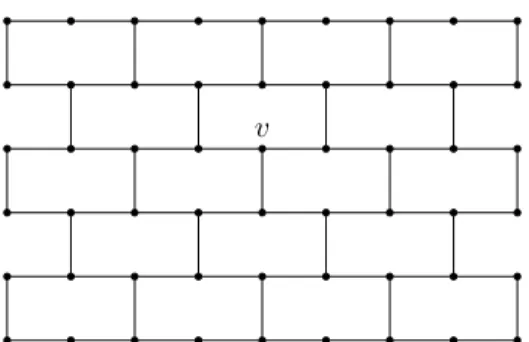
Figure 4.4 A more convenient drawing of the hexagonal lattice. . . 31
Figure 4.5 The truncated square lattice,T. . . 35
Figure 4.6 A more convenient drawing of the truncated square lattice. . . 36
Figure 4.7 A packing 7-coloring of G08,6, which can be used to tileT. . . 38
Figure 5.1 The two possible configurations of a 2-vertex. . . 41
Figure 5.2 More reducible configurations. . . 42
Figure 5.3 Precolored vertices added to reducible configurations. . . 43
Figure 5.4 Partial precolorings on these graphs are extended to prove that C3,1 is reducible. . . 43
Figure 6.1 The only coloring ofG−C that cannot be extended to G. . . 49
Figure 6.2 Rules for coloring the cycleC. . . 50
Figure 6.3 Two cycles C1 and C2 sharing a path, where uivj ∈/ E(G) for any k+ 1≤i≤nand k+ 1≤j≤n. . . 51
Figure 7.1 A counterexample to Conjecture3. . . 54
Figure 7.2 More counterexamples to Conjecture3. . . 55
Figure 7.3 An example of a cut vertex v incident with F where one component of G−v is drawn inside another. . . 57
Figure 7.4 An example of a chord uv on C where one component of G− {u, v} is drawn inside another. . . 58
Figure 7.5 A non-precolored 2-vertexv on the outer face ofG. . . 59
Figure 7.6 A non-precolored 3-vertexv on the outer face ofG. . . 60
Figure 7.7 A precolored pathP consisting of two 2-vertices. . . 61
ACKNOWLEDGEMENTS
I would like to thank Jen for gently pushing me to quit procrastinating and for believing in me unconditionally. I would like to thank Bernard for not-so-gently pushing me to quit procrastinating and for not giving up on me when graduating seemed like an impossible task.
ABSTRACT
In this thesis, we focus on variants of the coloring problem on graphs. A coloring of a graph Gis an assignment of colors to the vertices. A coloring is proper if no two adjacent vertices are assigned the same color. Colorings are a central part of graph theory and over time many variants of proper colorings have been introduced. The variants we study are packing colorings, improper colorings, and facial unique-maximum colorings.
A packing coloring of a graph G is an assignment of colors 1, . . . , k to the vertices of G such that the distance between any two vertices that receive color i is greater than i. A (d1, . . . , dk)-coloring of G is an assignment of colors 1, . . . , k to the vertices of G such
that the distance between any two vertices that receive coloriis greater thandi. We study
packing colorings of multi-layer hexagonal lattices, improving a result of Fiala, Klavˇzar, and Lidick´y [14], and find the packing chromatic number of the truncated square lattice. We also prove that subcubic planar graphs are (1,1,2,2,2)-colorable.
Afacial unique-maximum coloringofGis an assignment of colors 1, . . . , kto the vertices of Gsuch that no two adjacent vertices receive the same color and the maximum color on a face appears only once on that face. We disprove a conjecture of Fabrici and G¨oring [12] that plane graphs are facial unique-maximum 4-colorable. Inspired by this result, we also provide sufficient conditions for the facial unique-maximum 4-colorability of a plane graph. A {0, p}-coloring of Gis an assignment of colors 0 andp to the vertices ofGsuch that the vertices that receive color 0 form an independent set and the vertices that receive colorp form a linear forest. We will explore{0, p}-colorings, an offshoot of improper colorings, and prove that subcubic planarK4-free graphs are{0, p}-colorable. This result is a corollary of
a theorem by Borodin, Kostochka, and Toft [6], a fact that we failed to realize before the completion of our proof.
CHAPTER 1. INTRODUCTION
Graph theory is an area of discrete mathematics with applications in a wide range of fields, including computer science, sociology, and chemistry. The concept of graph coloring was introduced in order to solve the problem of coloring countries on a map so that no two countries that shared a border received the same color. This most basic variant of graph coloring, known as a proper coloring, is a key concept in modern graph theory. Indeed, the cornerstone of the theory of proper graph colorings, the Four Color Theorem [2], is one of the most famous results in all of graph theory. Proper colorings have been studied extensively, and with good reason. There is no shortage of applications of proper colorings, including scheduling, mobile networks, and Sudoku.
There are many other variants of graph coloring that have arisen from various appli-cations. We will present new results in packing colorings, improper colorings, and facial unique-maximum colorings.
In the next chapter, we will review basic terminology from graph theory and define the three graph coloring variants mentioned above.
In Chapter 3, we will establish methods used to prove results in later chapters. These include discharging, a well-known proof technique in graph coloring; linear/integer pro-gramming, an optimization modeling technique commonly used in industry and applied mathematics; boolean satisfiability, a modeling framework commonly used in computer sci-ence; and Thomassen’s precoloring method, which he used to prove that all planar graphs are 5-choosable [23].
In Chapters 4 and 5, we discuss packing colorings. Chapter 4 contains results on packing colorings of infinite lattices, in particular the hexagonal lattice and the truncated square lattice. This chapter is based on the manuscriptPacking chromatic numbers of multi-layer lattices by Messerschmidt [20].
In Chapter 5, we study (1,1,2,2,2)-colorings, a variant of packing colorings. In Chap-ter 6, we deal with a type of improper coloring called a {0, p}-coloring. In particular, we prove that planar subcubic graphs are (1,1,2,2,2)-colorable and planar subcubic K4-free
graphs are{0, p}-colorable.
In Chapter 7, we will study facial unique-maximum colorings. We will disprove a con-jecture on 4-color facial unique-maximum colorings and provide a condition for when a graph has a 4-color facial unique-maximum coloring. This chapter is based on the pub-lished paper A counterexample to a conjecture on facial unique-maximal colorings and the manuscriptOn facial unique-maximum colorings of plane graphsby Lidick´y, Messerschmidt, and ˇSkrekovski ([19] and [18])
Many of the proofs in this thesis make use of computer programs. These programs are available in the Appendix so that the interested reader can verify our results.
CHAPTER 2. DEFINITIONS
In this chapter, we will review graph theory terminology that is relevant to the topics in this thesis.
2.1 Basics
We denote the set of real numbers by Rand the set of integers byZ. We denote the set
{k∈Z: 1≤k≤n} by [n].
2.2 Graph theory
AgraphGis an ordered pair (V, E), where elements ofV are calledverticesand elements ofE, callededges, are two-element subsets ofV. We often useV(G) to denote the vertex set ofGandE(G) to denote the edge set ofG. We also use the notation uv as a shorthand for the edge{u, v}. A graphH is said to be a subgraph ofG, written H⊆G, if V(H)⊆V(G) and E(H) ⊆ E(G). A subgraph H of G is an induced subgraph of G if E(H) = {uv ∈ E(G) : u, v ∈ V(H)}. A subgraphH of Gis a proper subgraph of G if V(H) is a proper subset ofV(G) orE(H) is a proper subset ofE(G). GivenV0 ⊆V(G), the unique induced subgraph of G with vertex set V0 is denoted G[V0]. A simple graph G is a graph without
loops (edges from a vertex to itself) or multiedges (multiple edges between the same two
vertices).
Two verticesu, v∈V(G) areadjacent ifuv ∈E(G). The set N(v) ={u∈V(G) :uv∈ E(G)} is called the neighborhood ofv and the elements of N(v) are theneighbors of v. A vertex v and an edge e are incident if v ∈ e. We also say that two edges e1 and e2 are
incident if e1∩e2 6=∅. The degree of a vertexv, denoted deg(v), is the number of vertices
that are adjacent to v. We say v is a k-vertex if deg(v) = k, a k−-vertex if deg(v) ≤ k, and a k+-vertex if deg(v) ≥k. A graph G isk-regular if each vertex is a k-vertex. In this thesis, we will often refer to a graph ascubic if each vertex is a 3-vertex orsubcubic if each vertex is a 3−-vertex. An independent set is a subset S of the vertices such that no two vertices inS are adjacent.
A graphGis connected if, for any verticesu, v∈V(G), there exists a pathP ⊆Gthat contains u and v. If G is not connected, it is disconnected. A component of a graph G is a connected subgraph ofG that is not a proper subgraph of any connected subgraph ofG. In a connected graph G, a vertex v is a cut-vertex if G[V(G)\{v}] is disconnected. The distance between two vertices u, v∈V(G), denoted dist(u, v), is the length of the shortest pathP ⊆Gthat containsu andv. We define the distance between two vertices in different components to be∞.
A walk is a sequence v1v2· · ·vk of (not necessarily distinct) vertices in a graph such
that vi is adjacent to vi+1 for 1 ≤ i < k. A path is a walk with no repeated vertices.
A cycle is a path with an extra edge between the endpoints. A chord of a cycle C is
an edge not in E(C) that connects two vertices in V(C). A graph is complete if each vertex is adjacent to every other vertex. We denote the path on n vertices by Pn, the
cycle on n vertices by Cn, and the complete graph on n vertices by Kn. See Figure 2.1
for examples of these basic graphs. A tree is a connected graph that contains no cycles as subgraphs. A forest is a graph whose components are trees. A linear forest is a graph whose components are paths. Given a graph G, the subdivision of G, denoted S(G), is formed by replacing each edge uv ∈ E(G) with a new vertex w and two new edges uw and vw. Given two graphs G1 and G2, the Cartesian product of G1 and G2, denoted
G1G2, is the graph with vertex set {(v1, v2) : v1 ∈ V(G1), v2 ∈ V(G2)} and edge set
(a) (b) (c)
Figure 2.1 Examples of basic graphs with five vertices: (a) a path (P5), (b) a cycle (C5),
and (c) a complete graph (K5).
A graph is planar if it can be drawn in the plane without any edges crossing and a planar graph isplane if it is drawn in the plane in this manner. The edges of a plane graph partition the plane into contiguous regions calledfaces. A facef is said to beincident with the edges and vertices that form the boundary of f. Two faces are adjacent if they share an incident edge. Thelength of a facef, denoted`(f), is the number of edges that separate f from another face plus twice the number of edges around f that do not separate it from another face. The unbounded face of a plane graph is known as the outer face. We use F(G) to denote the set of faces of a plane graph G.
2.3 Graph coloring
Given a color set C, a coloring c:V(G) →C of a graph G is an assignment of colors to the vertices of G. The set of colors used in a graph coloring is usually [k]. We do not directly study proper colorings in this thesis, but the concept is central to the understanding of other coloring variants. A coloring isproper if any two adjacent vertices receive different colors. Ak-coloring of a graphGis a proper coloring usingkcolors andGisk-colorableif it has a k-coloring. Figure2.2(a) shows an example of a 2-coloring of P3P3. Thechromatic
A list assignment of a graphGis a function L:V(G)→2C that assigns to each vertex
a list of colors from C. An L-coloring of G is a proper coloring of G where each vertex v receives a color from its list L(v). A graph G is L-colorable if it has an L-coloring for a particular list assignment L. Figure 2.2(b) shows an example of a list assignment L on P3P3 and an L-coloring of that graph. We say that G is k-choosable if it is L-colorable
for any list assignment L such that |L(v)| ≥ k for all v ∈ V(G). The choosability of G, denoted ch(G), is the smallest k such that G is k-choosable. If a graph isk-choosable, it is k-colorable. After all, a proper coloring is just a list coloring where each vertex receives the same list. On the other hand,K2,4 is an example of a graph that is 2-colorable but not
2-choosable.
2.3.1 Packing coloring
Given a graph G, an i-packing is a set X ⊆ V(G) such that dist(u, v) > i for any u, v∈X. Apacking k-coloring is a partition ofV(G) into disjoint color classesX1, . . . , Xk
such that Xi is an i-packing for 1 ≤i ≤k. Figure 2.2(c) shows an example of a packing
4-coloring of P3P3. The packing chromatic number of G, denoted χρ(G), is the smallest
k such that G has a packing k-coloring. This type of coloring was originally inspired by the frequency assignment problem, which seeks to optimally assign broadcast frequencies to radio stations in order to limit interference between signals with the same frequency. It was introduced by Goddard et al. [16] under the name broadcast chromatic number, which underscored the original motivation. The termpacking chromatic number was first used by Breˇsar, Klavˇzar, and Rall in [7]. We also study a generalization of packing colorings. A (d1, . . . , dk)-coloring φ :V(G) → {φi}i∈[k] of a graph G is a coloring such that the set of
vertices that receive color φi forms a di-packing. By this definition packing k-coloring is
2.3.2 Improper coloring
A (d1, . . . , dk)-improper-coloring of a graph G is a partition ofV(G) into disjoint color
classes X1, . . . , Xk such that each vertex in Xi has at most di neighbors in Xi. In the
literature (see Choi and Esperet [10]), these colorings are simply referred to as (d1, . . . , dk
)-colorings, or more generally as improper colorings. However, we use the term (d1, . . . , dk
)-improper-coloring to distinguish this type of coloring from the packing coloring variant. A (0,2)-improper-coloring of a graph G would partition V(G) into sets V0 and V2 such that
V0 is an independent set and G[V2] consists of paths and cycles. We define a slightly more
restrictive variation on the (0,2)-improper-coloring. A {0, p}-coloring of a graph G is a partition of V(G) into sets V0 and Vp such that V0 is an independent set and G[Vp] is a
linear forest. Figure 2.2(d) shows an example of a{0, p}-coloring of P3P3.
2.3.3 Facial unique-maximum coloring
Afacial unique-maximumk-coloring of a plane graphGis a proper coloringc:V(G)→ [k] such that, for each facef ∈F(G), there exists a vertexv onF such thatc(v)> c(u) for all vertices u 6=v on f. We often use FUM-coloring as an abbreviation of the term facial unique-maximum coloring. Figure 2.2(e) shows an example of a FUM 4-coloring ofP3P3.
The FUM-chromatic number of G, denoted χfum(G), is the smallest k such that G has a
FUMk-coloring. This concept was introduced by Fabrici and G¨oring [12], who conjectured a stronger version of the Four Color Theorem.
1 2 1 2 1 2 1 2 1 1 3 2 3 2 1 2 1 3 {1,2} {1,3} {2,3} {1,3} {2,3} {1,2} {2,3} {1,2} {1,3} 3 1 2 1 4 1 2 1 3 (a) (b) (c) p p 0 p 0 p 0 p p 1 2 1 2 3 2 1 2 4 (d) (e)
Figure 2.2 Various colorings of P3P3: (a) a proper coloring, (b) a list coloring, (c) a
packing coloring, (d) a {0, p}-coloring, and (e) a FUM-coloring. In (d), the thick edges represent edges inG[Vp]. In (e), the arrows point from each face to
CHAPTER 3. METHODS
In this chapter, we outline the various methods used to prove results in the subse-quent chapters: discharging, linear and integer programming, boolean satisfiability, and Thomassen’s precoloring method. We will then demonstrate each method by proving a simple theorem.
3.1 Discharging
Discharging was developed by Wernicke in 1904 [25] in an attempt to prove the Four Color Theorem. Discharging seeks to quantify the general fact that planar graphs cannot have too many faces with high length and too many vertices with high degree.
A discharging proof is usually a proof by contradiction. We assume that our result is false and take G to be a minimum counterexample; that is, among all graphs which contradict the result,Ghas the smallest possible number of vertices.
We apply charge to the vertices and faces of Gusing the functionµ:V(G)∪F(G)→R
defined by µ(v) = adeg(v) −b for all v ∈ V(G) and µ(f) = (−1
2b−a)`(f) −b for all
f ∈F(G), wherea, b >0. Recall three well-known formulas in graph theory:
• |V(G)| − |E(G)|+|F(G)|= 2 (Euler’s Formula)
• P
v∈V(G)deg(v) = 2|E(G)| (Handshaking Lemma)
• P
Using these formulas, we can show that the total charge on the vertices and faces of Gis X v∈V(G) µ(v) + X f∈F(G) µ(f) = X v∈V(G) adeg(v)−b + X f∈F(G) −1 2b−a `(f)−b = 2a|E(G)| −b|V(G)|+ 2 −1 2b−a |E(G)| −b|F(G)| =−b |V(G)| − |E(G)|+|F(G)| =−2b <0.
We then construct rules which preserve charge while redistributing it so that each vertex and face has nonnegative charge. To make this easier, we often rule out certain subgraphs ofGcalledreducible configurations using our assumptions aboutG. Since total charge was initially negative but becomes nonnegative after redistribution, we have a contradiction.
We demonstrate the discharging method by proving the theorem for which Wernicke initially developed the method.
Theorem 1 (Wernicke [25]). If G is a planar graph with minimum degree 5, then there exists an edge uv ∈E(G) such thatdeg(u) = 5 and 5≤deg(v)≤6.
Proof. Suppose that the statement is false. Let G be a counterexample with the smallest
possible number of vertices. Arbitrarily add as many edges as possible to G while main-taining its planarity. This will result in a new graph G0 whose faces are all length 3. An edge is light if one endpoint is a 5-vertex and the other is a 5- or 6-vertex. Each vertex in G is a 5+-vertex, so any vertex incident to a new edge is a 6+-vertex in G0. Hence, if G0 contains a light edge, that edge must have been inG.
Apply charge µ(v) = deg(v)−6 to each vertex v∈V(G0) andµ(f) = 2`(f)−6 to each facef ∈F(G0). We verify that this charge function will result in a negative initial charge:
X v∈V(G0) µ(v) + X f∈F(G0) µ(f) = X v∈V(G0) deg(v)−6 + X f∈F(G0) 2`(f)−6 = 2|E(G0)| −6|V(G0)|+ 4|E(G0)| −6|F(G0)| =−6 |V(G0)| − |E(G0)|+|F(G0)| =−12.
We now proceed to the discharging phase of the proof. Redistribute charge throughout G0 according to the following rule:
(R1) Each 5-vertex takes charge 15 from each of its neighbors.
Finally, we show that each vertex and face in G0 has nonnegative final charge, thus deriving our contradiction. Each face in G0 is a triangle, so each face has charge 0. Each 5-vertex began with charge −1 and took charge 15 from each of its neighbors. Since two 5-vertices cannot be adjacent, each 5-vertex has final charge 0. Letvbe a 6+-vertex. Since vhad initial charge deg(v)−6 and gave charge 15 to each degree 5 neighbor, the final charge of v is at least 45deg(v)−6. We immediately see that if v is an 8+-vertex, it must have
positive charge. Ifv is a 6-vertex, then it cannot be adjacent to a 5-vertex, thusvhas final charge 0. If v is a 7-vertex, then it would need to be adjacent to at least six 5-vertices to have a negative final charge. This would require that two of these vertices be incident to the same face, and since each face ofG0 is a triangle, those two 5-vertices would have to be adjacent, which is impossible.
We have thus shown that, while the total initial charge on G0 was negative and no charge was created or destroyed, each face and vertex has nonnegative final charge. This is a contradiction, therefore no counterexample exists.
3.2 Linear and integer programming
Linear programming is a method of modeling an optimization problem using linear relationships. It was developed by George Dantzig in 1947 for the U.S. Air Force and has since been used extensively in industry. Given a system with parameters X1, . . . , Xn, we
seek to maximize or minimize the linear objective function Pn
i=1ciXi subject to a set of
linear constraints of the form Pn
j=1ai,jXj ≤ bi. Each linear constraint represents a
half-space in Rn and the set of feasible solutions is the intersection of these half-spaces, which
is a convex polyhedron. An optimal solution, if one exists, will occur at a vertex of the polyhedron.
An integer program is a linear program with a single added constraint: Xi ∈Z for all
i. While all linear programs are solvable in polynomial time, solving an integer program is NP-hard, even when Xi ∈ {0,1} for alli.
Below, we use integer programs to produce a simple result on the packing chromatic number ofP3P3.
Theorem 2. χρ(P3P3) = 4.
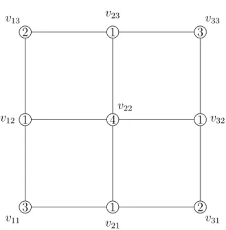
Proof. The proof consists of two integer programs: one exhibiting a packing 4-coloring of P3P3, shown in Figure3.1, and one showing that no packing 3-coloring of P3P3 exists.
First, we will show that no packing 3-coloring exists. Specifically, we will show that if three colors are used, we can cover at most eight vertices. Let Xijk be a binary variable
representing whether vertexvij can receive colork. We require that each vertex can receive
at most one color. For each 1≤i, j≤3, we add the constraint Xij1+Xij2+Xij3≤1.
We also need to enforce the distance restriction. For each color kand each pair of vertices u, v such that dist(u, v)≤k, at most one of u and v can receive colork.
3 1 2 1 4 1 2 1 3 v11 v12 v13 v21 v22 v23 v31 v32 v33
Figure 3.1 P3P3 with an example of an optimal packing.
For v11 for example, we have the following constraints:
X111+X121≤1 X112+X122≤1 X113+X123≤1 X111+X211≤1 X112+X212≤1 X113+X213≤1 X112+X132≤1 X113+X133≤1 X112+X222≤1 X113+X23≤1 X112+X312≤1 X113+X313≤1 X113+X233≤1 X113+X323≤1
The final integer program is Maximize X i,j,k∈{1,2,3} Xijk Subject toX111+X112+X113 ≤1 .. . X331+X332+X333 ≤1 X111+X121≤1 .. . X323+X333≤1 Xijk∈ {0,1} fori, j, k ∈ {1,2,3}
We enter this integer program into Sage’sMixedIntegerLinearProgramfunction and solve it using Sage’s built-in GLPK solver. The result is that the maximum value of the objective function is 8. SinceP3P3has nine vertices, no packing 3-coloring exists. Next, we construct
a similar integer program to try and find a packing 4-coloring ofP3P3:
Maximize X i,j∈{1,2,3} k∈{1,2,3,4} Xijk Subject toX111+X112+X113+X114≤1 .. . X331+X332+X333+X334≤1 X111+X121≤1 .. . X324+X334≤1 Xijk∈ {0,1} fori, j∈ {1,2,3}, k∈ {1,2,3,4}
The objective function achieves a maximum of 9 with the following solution: X111= 0 X112= 0 X113 = 1 X114= 0 X121= 1 X122= 0 X123 = 0 X124= 0 X131= 0 X132= 1 X133 = 0 X134= 0 X211= 1 X212= 0 X213 = 0 X214= 0 X221= 0 X222= 0 X223 = 0 X224= 1 X231= 1 X232= 0 X233 = 0 X234= 0 X311= 0 X312= 1 X313 = 0 X314= 0 X321= 1 X322= 0 X323 = 0 X324= 0 X331= 0 X332= 0 X333 = 1 X334= 0
These variable assignments can be interpreted as the packing coloring shown in Figure 3.1. Since P3P3 has a packing 4-coloring but no packing 3-coloring,χρ(P3P3) = 4.
3.3 Boolean satisfiability
A boolean satisfiability problem is a logical statement consisting of boolean variables. If there exist values for each variable such that the entire statement evaluates to true, the problem is satisfiable. If no such set of values exists, then the problem is unsatisfiable. A literal is a single boolean variable or its negation. A clause is a statement consisting of literals separated by logical ORs. A boolean satisfiability problem is in conjunctive normal form if it consists of clauses separated by logical ANDs. The boolean satisfiability problem is one of the classic NP-complete problems, however many efficient heuristics have been developed to solve boolean satisfiability problems in conjunctive normal form.
Inspired by Chen, Martin, Martin, and Raimondi [9], we provide another proof of The-orem 2 by constructing boolean satisfiability problems.
Proof of Theorem 2. We proceed by proving that no packing 3-coloring exists and finding
whether vertex vij can receive color k. First, we require that each vertex receive a color.
For each vertexvij, we add the clauseXij1∨Xij2∨Xij3. Then, for each colork and each
pair of vertices u, v such that dist(u, v) ≤ k, if one of these vertices receives color k, the other does not. For vertexv11 for example, we add the following clauses:
¬X111∨ ¬X121 ¬X112∨ ¬X122 ¬X113∨ ¬X123 ¬X111∨ ¬X211 ¬X112∨ ¬X212 ¬X113∨ ¬X213 ¬X112∨ ¬X132 ¬X113∨ ¬X133 ¬X112∨ ¬X222 ¬X113∨ ¬X23 ¬X112∨ ¬X312 ¬X113∨ ¬X313 ¬X113∨ ¬X233 ¬X113∨ ¬X323
The final boolean satisfiability problem is
(X111∨X112∨X113)∧ · · · ∧
(X331∨X332∨X333)∧
(¬X111∨ ¬X121)∧
(¬X112∨ ¬X122)∧ · · · ∧
(¬X323∨ ¬X333).
Entering this formula into the Glucose SAT solver [3] reveals that the problem is unsatisfi-able, thus no packing 3-coloring ofP3P3 exists.
4-coloring ofP3P3: (X111∨X112∨X113∨X114)∧ · · · ∧ (X331∨X332∨X333∨X334)∧ (¬X111∨ ¬X121)∧ (¬X112∨ ¬X122)∧ · · · ∧ (¬X324∨ ¬X334)
Glucose determines that this problem is satisfiable and provides a solution:
X111= 0 X112= 0 X113 = 1 X114= 0 X121= 1 X122= 0 X123 = 0 X124= 0 X131= 0 X132= 1 X133 = 0 X134= 0 X211= 1 X212= 0 X213 = 0 X214= 0 X221= 0 X222= 0 X223 = 0 X224= 1 X231= 1 X232= 0 X233 = 0 X234= 0 X311= 0 X312= 1 X313 = 0 X314= 0 X321= 1 X322= 0 X323 = 0 X324= 0 X331= 0 X332= 0 X333 = 1 X334= 0
These variable assignments can be interpreted as the packing coloring shown in Figure 3.1. Since P3P3 has a packing 4-coloring but no packing 3-coloring,χρ(P3P3) = 4.
3.4 Thomassen’s precoloring method
This technique was developed by Thomassen [23] in order to prove the following result.
Theorem 3 (Thomassen [23]). All planar graphs are 5-choosable.
Theorem 3 is a corollary of the slightly stronger result in Theorem 4. Thomassen’s method is best demonstrated by proving Theorem4, which it was originally developed for.
Theorem 4 (Thomassen [23]). Let G be a graph with list assignment L such that
• there is a pathP with at most two vertices on the outer face such that the vertices in P have distinct lists of size 1,
• every other vertex on the outer face has at least three colors in its list, and • every vertex not on the outer face has at least five colors in its list.
Then Gis L-colorable.
Proof. Suppose for contradiction that G is a counterexample with the minimum number
of vertices and L is its corresponding list assignment. We refer to the vertices in P as precolored vertices since we have no choice in which color they receive. We first prove that the outer face of Gis bounded by an induced cycle.
We may assume that G is connected, otherwise by the minimality of G we could color each component separately. Suppose G has a cut-vertex v. Let G1 and G2 be induced
subgraphs of G such that V(G1)∪V(G2) = V(G) and V(G1)∩V(G2) = {v}. Assume
without loss of generality that a, b ∈ V(G1). By the minimality of G, there exists an L
-coloring c1 of G1. Let L0 be a list assignment on G2 such that L0(v) = {c1(v)} and L0 is
equal to L on V(G2)\{v}. Since L0 meets the criteria of a list assignment laid out in the
theorem (v is the precolored vertex), we can find anL0-coloring c2 of G2 that agrees with
c1 on v. Extending the colorings c1 and c2 to the entire graph yields anL-coloring. This is
a contradiction, thus Gcannot have a cut-vertex.
Since Gis connected and has no cut-vertices, the outer face of Gmust be bounded by a cycleC. Suppose thatC is not an induced cycle; that is,C has a chorduv. LetG1 andG2
be induced subgraphs ofGsuch that V(G1)∪V(G2) =V(G) andV(G1)∩V(G2) ={u, v}.
Assume without loss of generality thata, b∈V(G1). We can again find anL-coloringc1 of
G1 by the minimality of G. Let L0 be a list assignment on G2 such that L0(u) = {c1(u)},
an L0-coloring c2 of G2 that agrees withc1 on u and v. We extend c1 and c2 to the entire
graph to again get a contradiction, thusC must be an induced cycle.
If P contains no vertices, arbitrarily pick a vertex and reduce its list to one color, then redefine P to contain that vertex. Leta be one of the vertices in P. Let x and y be adjacent vertices on the outer face such thatxis adjacent toaandx /∈V(P). LetCbe a set consisting of two colors from L(x) not in L(a). Let G0 =G[V(G)\{x}], N =N(x)\{a, y}, and L0 be a list assignment on G0 such that L0(v) = L(v)\C if v ∈ N and L0(v) = L(v) otherwise. By the minimality of G, there exists an L0-coloringc of G0. Since y is the only neighbor of x that could have received one of the two colors in C, we can extend c to x, thus coloring the entire graph. This is a contradiction, therefore no counterexample exists.
P N
G−C x
y a
Figure 3.2 An example of a graph Gwith outer face bounded by an induced cycle. Note thaty /∈V(P) in this example, which need not be the case.
CHAPTER 4. PACKING COLORING OF GRIDS
This chapter is based onPacking chromatic numbers of multi-layer lattices [20], a paper in preparation for submission.
4.1 Introduction
The packing chromatic number of the square lattice Z2 is a major problem and has
already been studied extensively. Goddard, Harris, Hedetniemi, Hedetniemi, and Rall [16] showed that the packing chromatic number ofZ2 is between 9 and 23. Later, Fiala, Klavˇzar,
and Lidick´y [14] improved the lower bound to 10 while Holub and Soukal [17] improved the upper bound to 17. Finally, Chen, Martin, Martin, and Raimondi [9] improved the lower bound further to 13 and the upper bound to 15, which is where both bounds remain. Finbow and Rall [15] showed thatZ3 (orZ2Z) does not have a finite packing. This brings about a
natural question: for whichn∈N∪ {∞}doesχρ(Z2Pn) jump to infinity? Fiala, Klavˇzar,
and Lidick´y [14] showed that the answer to this question is 2.
In [14], Fiala, Klavˇzar, and Lidick´y also derived two results on the hexagonal latticeH. They showed that χρ(H) = 7 and χρ(HPn) =∞ for alln≥6. Left as an open question
was for whichndoes χρ(HPn) make the jump to infinity. We respond with the following
conjecture.
Conjecture 1. The smallest value of nsuch that χρ(HPn) =∞ is 3.
Recently, Moss [21] proved that χρ(HP2) ≤ 205. Our main result is the following
Theorem 5. For n≥4, χρ(HPn) =∞, where H is the infinite hexagonal lattice.
We also provide a lower bound for χρ(HP3). Theorem 6. χρ(HP3)>346.
While we could not prove that HP3 does not have a finite packing, we believe that
Theorem6 strongly suggests that Conjecture 1is true.
Inspired by the hexagonal lattice, we studied another cubic lattice, the truncated square latticeT, shown in Figure4.5. We determined its packing chromatic number exactly.
Theorem 7. χρ(T) = 7, where T is the truncated square lattice.
The proof of Theorem 5 will introduce a new method involving integer and linear pro-grams for determining packing chromatic numbers. Theorem7is proved using SAT solvers, a technique developed by Chen, Martin, Martin, and Raimondi [9].
In the next section, we prove Theorem5. Section4.3describes the proof of Theorem7.
4.2 Hexagonal lattices 4.2.1 4 layers
The main topic of this section is the proof of Theorem 5. In order to prove Theorem5, we will first need to establish some concepts related to packing density.
LetXi be the set of vertices in a graph receiving colori. In a finite graphG, the density
of Xi, denoted d(Xi), would simply be defined as |V|X(Gi|)|. Since |V(HP4)|= ∞, we need
to tweak the definition slightly. Let Hi be the induced subgraph of H on the vertex set
{u ∈V(H) : dist(u, v) ≤i}. SinceH is vertex transitive, the choice of v in this definition is irrelevant. For the purpose of packing colorings on HP4, define the density of Xi as
lim supi→∞ |Xi∩V(HiP4)|
Lemma 1. Given a subgraph G of H, if M is an upper bound for dGP4(Xi), then M is
also an upper bound for dHP4(Xi).
Proof. Suppose dHP4(Xi)> M. Since each vertex in HP4 appears in an equal number
of copies ofGP4,dHP4(Xi) is bounded above by the average of the density of Xi over all
isomorphic copies of GP4 inHP4. This would require that the density ofXi in at least
one copy of GP4 be greater thanM, which is a contradiction.
We use Lemma 1 to establish density bounds in the next two lemmas.
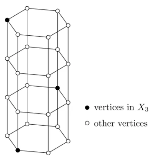
Lemma 2. d(X3)≤ 18.
Proof. Consider the subgraph C6P4 (see Figure4.1). If a layer of this subgraph contains
a vertex fromX3, there is only one location in the adjacent layer that can contain a vertex
fromX3 (the opposite corner of the hex). However, three consecutive layers cannot contain
a vertex fromX3. It is therefore only possible to have three vertices fromX3 inC6P4, for
a maximum density of 18.
vertices inX3
other vertices
Figure 4.1 An example of a packingX3 of C6P4 with density 18.
We will now use an integer programming method to bound the density of colors 1, 2, and 4.
Lemma 3. d(X1∪X2∪X4)≤ 23.
Figure 4.2 A subgraph H⊆ H used to bound d(X1∪X2∪X4).
Proof. Let H be the subgraph of H shown in Figure 4.2. Consider the graph HP4. For
each v∈V(HP4) andi∈ {1,2,4}, letYv,i be a binary variable that represents whetherv
can receive color i. Each vertexv can only receive one color, giving us the constraint Yv,1+Yv,2+Yv,4 ≤1 for all v∈V(HP4).
The distance restriction gives us the following three constraints: Yv,1+Yu,1 ≤1 for all u, v∈V(HP4) s.t. dist(u, v) = 1
Yv,2+Yu,2 ≤1 for all u, v∈V(HP4) s.t. 1≤dist(u, v)≤2
Hence, the largest packing of HP4 with colors 1, 2, and 4 can be found by solving the
following integer program:
Maximize X
v∈V(HP4) i∈{1,2,4}
Yv,i
Subject to Yv,i∈ {0,1}for all v∈V(HP4), i∈ {1,2,4}
Yv,1+Yu,1 ≤1 for all u, v∈V(HP4) s.t. dist(u, v) = 1
Yv,2+Yu,2 ≤1 for all u, v∈V(HP4) s.t. 1≤dist(u, v)≤2
Yv,4+Yu,4 ≤1 for all u, v∈V(HP4) s.t. 1≤dist(u, v)≤4 X
i∈{1,2,4}
Yv,i ≤1 for allv∈V(HP4).
The solution to this integer program is 64. Since HP4 has 96 vertices, this works out to
a density of 23, which is an upper bound ford(X1∪X2∪X4) by Lemma1.
We use weight functions to find bounds on density for the remaining colors. Given a vertexv∈Xi, aweight functionwv :V →[0,1] assigns a weight to the vertices aroundvin
the hope that no vertex receives total weight greater than 1 from all vertices inXi. Given
a weight function wv, thearea A covered byv is Pu∈V wv(u).
The bounds for colors 5 and 6 are calculated using a linear programming method that takes into account interaction between vertices in different layers that share the same color.
Lemma 4. d(X6)≤0.0273
Proof. Given a vertex v, let
wv(u) = 1, dist(u, v)≤3 0, otherwise.
Notice that a packing X6 is valid only if for each u ∈ HP4,Pv∈X6wv(u) ≤1. Letdi
be the density of color 6 in layeriand letAi,j be area in layericovered by a vertex in layer
j. Finding an upper bound ford(X6) is equivalent to maximizing 14(d1+d2+d3+d4). We
can bounddi above by
1 Ai,i 1− X 1≤j≤4 j6=i Ai,jdj .
Using the formula
Ai,j = 19, i=j 10, |i−j|= 1 4, |i−j|= 2 1, |i−j|= 3 for color 6, we have the following linear program:
Maximize 14(d1+d2+d3+d4)
Subject to di∈[0,1] for alli∈ {1,2,3,4}
d1≤ 191(1−10d2−4d3−d4)
d2≤ 191(1−10d1−10d3−4d4)
d3≤ 191(1−4d1−10d2−10d4)
d4≤ 191(1−d1−4d2−10d3)
The solution to this linear program gives us d(X6)≤0.0273. Lemma 5. d(X5)≤0.0417.
Proof. We again wish to construct a weight function that captures the area covered by color 5. Constructing this function for color 5 presents a greater challenge than for color 6. Our goal is to maximize the total weight given to each vertex while maintaining the property that each vertex receives a total weight no greater than 1. We could use a binary weight function like the one used in Lemma 4, but we can do better if we deal with distance 3 vertices as a special case.
Let u be a vertex in layer 1 or 4. There exist configurations in which there are four vertices from X5 that are distance 3 from u. However, there also exists configurations in
which there are three vertices from X5 that are distance 3 from u and a fourth cannot be
added. To account for this, we define a new function to help us maximize the total weight given to the vertices.
Given vertices u and v with dist(u, v) =d, let nv(u) be the number of neighbors x of
v such that there is a path of length dbetween v and u that passes throughx. Let uv be
the vertex in the same layer asvthat is closest tou (whereuv =uifuis in the same layer
as v) and define n`v(u) := nv(uv). Let wv :V(HP4) → [0,1] be the function defined as
follows:
• if dist(v, u)<3,wv(u) = 1
• if dist(v, u) = 3 and uis in layer 2 or 3, then wv(u) = 13n`v(u)
• if dist(v, u) = 3 and uis in layer 1 or 4, then wv(u) = 14nv(u)
• if dist(v, u)>3,wv(u) = 0
Claim 1. If X5 is a valid packing, then Pv∈X5wv(u)≤1 for allu∈V.
Proof. Letuandvbe vertices inHP4, wherev∈X5. If dist(u, v)<3, then we must have
dist(u, v0) > 3 for any v0 ∈ X5\{v}, in which case v0 contributes no weight tou. Assume
then that dist(u, v) = 3.
Suppose there exists a neighbor xof usuch thatxlies on a path of length 3 connecting u and v and a path of length 3 connecting u and some v0 ∈X5\{v}. Then there is a path
of length 2 connecting v and x and a path of length 2 connecting v0 and x. This gives dist(v, v0) ≤ 4, which is a contradiction. Hence, for each neighbor x of u, there must be only one vertex in X5 which is connected tou by a path of length 3 that passes throughx.
Consequently, deg(u) is an upper bound on the number of distance 3 neighbors ofu from X5.
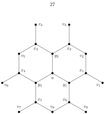
u y3 x5 v8 x6 y1 x1 v2 x2 y2 x3 v5 x4 v1 v3 v4 v6 v7 v9
Figure 4.3 Since x1 and x2 both lie on length 3 paths between v2 and u, nv2(u) = 2.
On the other hand, x1 is the only neighbor of v1 that lies on a length 3 path
betweenv1 andu, sonv1(u) = 1. Notice thatv1,v4, andv7 could all be in X5,
but if insteadv2 ∈X5, then only one other vi could be inX5.
If u is in layer 1 or 4, deg(u) = 4. For each v ∈ X5 at distance 3 from u with nv(u)
we reduce by one the maximum number of vertices from X5 that can be distance 3 from
u. Hence, u can receive 12 weight from two vertices, or 12 from one vertex and 14 from up to two vertices, or 14 from up to four vertices.
If u is in layer 2 or 3, deg(u) = 5. If v is not in the same layer as u, the only way that nv(u) = 1 is ifv is three layers away fromu, which is impossible. We can thus have at most
three vertices in X5 at distance 3 from u: one for each neighbor of u in the same layer as
u. We ignore the neighbors of u in adjacent layers and use the function n`
v to determine
the contribution of v. If n`v(u) = 2, then there can be at most one more vertex from X5
at distance 3 from u, so u receives 23 weight from v and at most 13 additional weight. If n`
v0(u) = 1 for allv0 ∈X5 that are distance 3 fromu, thenu receives 13 from at most three
Let di be the density of color 5 in layer i. Each vertex in layer 2 that receives color 5
covers an area of 7 in layer 1, while each such vertex in layer 3 covers 52 in layer 1 and each such vertex in layer 4 covers 14 in layer 1. In total, the area in layer 1 covered by vertices outside of layer 1 is 7d2+52d3+14d4. Each vertex in layer 1 that receives color 5 covers an
area of 13 in layer 1, thus d1 ≤ 131 1−7d2− 52d3−14d4
. Using similar bounds for d2, d3,
and d4, we construct the following linear program:
Maximize 14(d1+d2+d3+d4)
Subject to di ∈[0,1] for alli∈ {1,2,3,4}
d1 ≤ 131(1−7d2−52d3−14d4)
d2 ≤ 141(1−6d1−6d3−2d4)
d3 ≤ 141(1−2d1−6d2−6d4)
d4 ≤ 131(1− 14d1−52d2−7d3)
The solution to this linear program gives us d(X5)≤0.0417.
Lemma 6. Fork≥4, the density of X2k is bounded above by 6k2−121k+16.
Proof. Given a vertex v inH, the number of vertices at distance kfrom v is 3k, hence the number of vertices at distance at mostk, including v, is
1 + k X i=1 3i= 1 + 3(k+ 1)k 2 .
Summing over four layers, we have A(v) = k X i=k−3 1 + 3(i+ 1)i 2 = 6k2−12k+ 16, therefore d(X2k)≤ 6k2−121k+16.
We now have all of the bounds necessary to prove Theorem 5.
Proof of Theorem 5. Since d(Xi) decreases monotonically with i, we can use d(X6) as an
upper bound ford(X7) and d(X2k) as an upper bound ford(X2k+1). Thus, we have
∞ X k=8 d(Xk)≤2 ∞ X k=4 d(X2k) ≤2 ∞ X k=4 1 6k2−12k+ 16 ≤2 ∞ X k=4 1 6k2 ≤ 13 Z ∞ 3 1 k2dk = −1 3k −1 ∞ 3 = 1 9.
Given any packing coloring X1, . . . , Xn, the following inequality holds: n X k=1 d(Xk)≤ ∞ X k=1 d(Xk) ≤d(X1∪X2∪X4) +d(X3) +d(X5) +d(X6) +d(X7) + ∞ X k=8 d(Xk) ≤ 23 +1 8+ 0.0417 + 2·0.0273 + 1 9 <0.9992<1.
Hence, no finite packing ofHP4 exists. For anyn >4, the existence of a finite packing
of HPn would imply that a complete finite packing of HP4. Therefore, for any n≥4,
no finite packing ofHPn exists.
4.2.2 3 layers
We also provide a lower bound for χρ(HP3) using methods similar to those used to
Lemma 7. d(X3)≤ 19.
Proof. Consider the subgraphC6P3. No layer can contain two vertices from X3 and only
two layers of C6P3 can contain one vertex fromX3, henced(X3)≤ 19. Lemma 8. d(X1∪X2∪X4∪X8)≤ 4972.
Proof. LetH be the subgraph of Hin Figure4.2. Consider the graph HP3. We can find
the largest packing ofHP3 with colors 1, 2, 4, and 8 by solving an integer program similar
to the one in the proof of Lemma3:
Maximize X
v∈V(HP3) i∈{1,2,4,8}
Yv,i
Subject to Yv,i∈ {0,1}for all v∈V(HP3), i∈ {1,2,4,8}
Yv,1+Yu,1 ≤1 for all u, v∈V(HP3) s.t. dist(u, v) = 1
Yv,2+Yu,2 ≤1 for all u, v∈V(HP3) s.t. 1≤dist(u, v)≤2
Yv,4+Yu,4 ≤1 for all u, v∈V(HP3) s.t. 1≤dist(u, v)≤4
Yv,8+Yu,4 ≤1 for all u, v∈V(HP3) s.t. 1≤dist(u, v)≤8 X
i∈{1,2,4,8}
Yv,i ≤1 for allv∈V(HP3).
The solution to this integer program is 49, giving us a density of 4972.
Lemma 9. Given a vertexvinH, the number of verticesuwithdist(u, v) =dandnv(u) =
2 is 3bd−21c.
Proof. To make the hexagonal lattice easier to work with, we flatten it so that it more
closely resembles a subgraph of the square lattice (see Figure 4.4). The vertices of H can thus be expressed as elements ofZ2: V(H) ={(i, j) :i, j∈Z}.
Consider the vertex v from Figure 4.4. Let v = (0,0). Given a vertex u = (k, `), it is clear that nv(u) = 1 if`= 0, so we consider the cases when ` <0 and ` >0. Assume by
v
Figure 4.4 A more convenient drawing of the hexagonal lattice.
Claim 2. If ` <0, then nv(u) = 2 if and only if |`| −k≤ −1.
Proof. Clearly dist(u, v) = distZ2(u, v) =|`|+kif and only if|`| −k≤1. If|`| −k >1, then
any path fromvtouinZ2of length distZ2(u, v) must contain a subpath (i, j)(i, j−1)(i, j−2).
Since the path (i, j)(i, j−1)(i, j−2) does not exist in H, it must be replaced by either (i, j)(i+ 1, j)(i+ 1, j−1)(i, j−1)(i, j−2) or (i, j)(i, j−1)(i+ 1, j−1)(i+ 1, j−2)(i, j−2), depending on the parity of iandj. The minimum number of edge-disjoint subpaths of the form (i, j)(i, j−1)(i, j−2) in a uv-path inZ2 isb|`|−2kc, each of which increases distH(u, v) by 2. Hence, dist(u, v) =|`|+k+ maxn0,2j|`|−2kko. Note that this formula is only valid because uis below v and v is adjacent to the vertex directly below it.
If |`| −k≤ −1, then we can easily find two uv-paths of length dist(u, v), one of which passes through (1,0) and one of which passes through (0,−1). Suppose that |`| −k >−1. We will show that anyuv-pathP that passes through (1,0) does not have length dist(u, v). Assume that P begins with (0,0)(1,0)(2,0). If u = (0,−1), then clearly P does not have length dist(u, v); otherwise, |`| − |k−2| > −1. Since dist (2,0),(k, `)
= |`|+|k−2|+ maxn0,2j|`|−|2k−2|ko, the length ofP is 2 +|`|+|k−2|+ maxn0,2j|`|−|2k−2|ko.
Ifk <2, then |E(P)|=|`|+ 4−k+ max 0,2 |`| −2 +k 2 =|`|+ 2 + max 2−k,2 |`| −k 2 +k >|`|+k+ max 0,2 |`| −k 2 = dist(u, v). Ifk≥2, then |E(P)|=|`|+k+ max 0,2 |`| −k+ 2 2 >|`|+k+ max 0,2 |`| −k 2 = dist(u, v).
By Claim 2, for any vertexu= (k, `) with nv(u) = 2 and` <0, we have|k|+`≥1 and
dist(u, v) =|k| −`. Given a fixedd= dist(u, v), `≥1− |k|
≥1−(`+d)
≥ 1−d
2 .
This allows for bd−1
2 c values of `. Since k6= 0, each value of `corresponds to two possible
values ofk, hence there are 2bd−21c verticesu withnv(u) = 2 and` <0. Claim 3. If ` >0, then nv(u) = 2 if and only if k < `.
Proof. Since dist(u, v) =`+kif and only if`−k≤0, we can show that dist(u, v) =`+k+
max
0,2`−k+1
2 using an argument similar to that in Claim2. If` < k, then dist(u, v) =
`+k and clearly no uv-path that passes through (−1,0) or (0,−1) has length dist(u, v). Suppose ` ≥ k. The paths P1 = (0,0)(−1,0)(−1,1)(0,1) and P2 = (0,0)(1,0)(1,1)(0,1)
are twouv-paths of length 3 = dist (0,0),(0,1)
that pass through different neighbors ofv. Consider a (0,1)(k, `)-path of length dist (0,1),(k, `)
. We have dist (0,1),(k, `) =`−1 +k+ max 0,2 `−1−k 2 =`+k+ max 0,2 `+ 1−k 2 −3 = dist(u, v)−3,
hence we can constructuv-pathsP1∪P and P2∪P of length dist(u, v) that pass through
different neighbors ofv.
By Claim 3, for any vertex u = (k, `) with nv(u) = 2 and` > 0, we have |k|< ` and
dist(u, v) =`+|k|+ 2j`−|k2|+1k. If d= dist(u, v) is even, then d= 2`. Since |k|+` must be even and|k|< `, there are d/2−1 possible values ofk. If dis odd, thend= 2`+ 1. In this casek+`must be odd, so there are d−21 possible values ofk. Regardless of the parity of d, there is only one possible value of` and bd−1
2 c possible values of k. Therefore, there
are 3bd−21c verticesu withnv(u) = 2 in total.
Proof of Theorem 6. Letvbe a vertex inHP3in layeri. For each colorn≥5, we estimate
the density using a generalized weight function based on the parity ofn. Ifn= 2k, we use the weight function
wv(u) = 1, dist(u, v)≤k 0, otherwise to calculate the area function
Ai,j= 1 + 3
(k− |i−j|)(k− |i−j|+ 1)
Ifn= 2k+ 1, we use the weight function wv(u) = 1, dist(u, v)< k+ 1 1 3nv,i(u), dist(u, v) =k+ 1 0, otherwise.
to calculate the area function Ai,j = 3 (k− |i−j|)(k− |i−j|+ 1) 2 + 3(k− |i−j|) 2 + 2.
The verticesuin layerjwith dist(u, v)< k+1 contribute 1+3(k−|i−j|)(k2−|i−j|+1) toAi,j. By
Lemma9, there are 3bk−|2i−j|c verticesu in layer j with dist(u, v) =k+ 1 and nv,i(u) = 2,
each contributing 23 toAi,j. This leaves 3(k− |i−j|+ 1)−3bk−|2i−j|cvertices contributing 1
3. The total contribution of vertices in layerj at distance k+ 1 is
2 3 3 k− |i−j| 2 +1 3 3(k− |i−j|+ 1)−3 k− |i−j| 2 = 2 k− |i−j| 2 +k− |i−j|+ 1− k− |i−j| 2 = k− |i−j| 2 +k− |i−j|+ 1 = 3(k− |i−j|) 2 + 1. Using these values ofAi,j, we construct the linear program
Maximize 13(d1+d2+d3)
Subject to di∈[0,1] for alli∈ {1,2,3}
d1≤ A11,1(1−A1,2d2−A1,3d3)
d2≤ A12,2(1−A2,1d1−A2,3d3)
d3≤ A13,3(1−A3,1d1−A3,2d2),
These bounds and the bounds from Lemmas 7 and 8give us 347 X k=1 d(Xk)≤d(X1∪X2∪X4∪X8) +d(X3) + 7 X k=5 d(Xk) + 346 X k=9 d(Xk) < 49 72 + 1 9 + 0.095754 + 0.112577 <0.999996<1.
4.3 Truncated square lattices
Another infinite cubic graph that we studied was the truncated square lattice,T, shown in Figure 4.5. Our goal is to prove Theorem7, which states thatχρ(T) = 7.
Figure 4.5 The truncated square lattice,T.
We flatten T in the same fashion as H (see Figure 4.6) so that its vertices can be expressed as elements ofZ2.
Let m and n be positive integers such that 4 | m and 2 | n and let Vm,n = {(i, j) :
1 ≤i≤m,1 ≤j ≤n}, where vertex (1,1) is adjacent to (1,2). Take Gm,n = T[Vm,n]. If
χρ(T)≤M, then there must be a subgraph isomorphic toGthat has a packingM-coloring.
Conversely, ifGdoes not have a packingM-coloring, thenχρ(T)> M. Hence, our strategy
for finding a lower bound forχρ(T) is to find a large value of M such that χρ(Gm,n)> M
Figure 4.6 A more convenient drawing of the truncated square lattice.
To find an upper bound for χρ(T), we use use a similar strategy on a slightly modified
version ofGm,n. LetG0m,n be a graph with vertex set V(Gm,n) and edge set
E∪ {(1, j)(m, j) : 1≤j≤n} ∪ {(i,1)(i, n) : 1< i < m,degGm,n(i,1) = 2}.
Notice that this graph is designed to preserve adjacencies lost from cutting G out of the lattice. If G0m,n has a packing M-coloring, then T can be partitioned into copies ofGm,n,
each receiving the same packing coloring. Finding such a coloring, which we refer to as a tiling, would be sufficient to prove that χρ(Gm,n)< M. Hence, our strategy for finding an
upper bound for χρ(T) is to find a small value of M such that χρ(Gm,n) ≤ M for some
m, n.
To find these bounds, we make use of a SAT solver to solve a boolean satisfiability problem. Aboolean satisfiability problemis a logical statement made up of clauses separated by logical And (∧) operators. Each clause consists of literals – either boolean variables or their negations – separated by logical Or (∨) operators. We will reformulate the problem of calculating the packing chromatic number of an infinite graph as a satisfiability problem.
Let Xi,j,k be a boolean variable that represents whether vertex (i, j) can receive color
k. The problem of finding a packing`-coloring requires two constraints: • Each vertex must be able to receive at least one color: W
(i,j)∈Vm,nXi,j,k, 1≤k≤`. • Two vertices can only receive color kif they are at distance greater than k:
¬Xi1,j1,k∨ ¬X12,j2,k, (i1, j1),(i2, j2)∈Vm,n, 1≤k≤`, dist (i1, j1),(i2, j2)
≤k.
According to Chen, Martin, Martin, and Raimondi [9], the SAT solver program will run more efficiently if the large clauses from the first constraint are broken up into several smaller clauses. A large clause can be broken up into k+ 1 smaller clauses using k new variables known ascommander variables. For example, the clauseXi,j,1∨Xi,j,2∨· · ·∨Xi,j,m
can be broken up using the commander variables Ci,j,1, Ci,j,2, . . . , Ci,j,k as follows:
Xi,j,1∨ · · · ∨Xi,j,bm/kc∨ ¬Ci,j,1
∧
Xi,j,bm/kc+1∨ · · · ∨Xi,j,b2m/kc∨ ¬Ci,j,2∧
.. .
Xi,j,b(k−1)m/kc+1∨ · · · ∨Xi,j,m∨ ¬Ci,j,m
∧
(Ci,j,1∨ · · · ∨Ci,j,k)
Notice that if no Xi,j,k is true, then each ¬Ci,j,k must be true and thus the last clause
cannot be satisfied. It is not clear how best to break up large clauses, so we decided that a large clause containing mliterals would be broken up intob√mc+ 1 clauses usingb√mc commander variables.
Since T is vertex-transitive, we can precolor a single vertex of G0m,n when calculating an upper bound for χρ(T). If we are looking for a packing `-coloring of G0m,n, then we
precolor an arbitrary vertex with color` in order to reduce the number of clauses as much as possible. If a coloring using fewer than ` colors exists, then we can recolor any single vertex with `. If a coloring using exactly ` colors exists, then there exists such a coloring where any single arbitrary vertex receives color`.
We are now ready to prove Theorem 7.
Proof of Theorem 7. Using the satisfiability problem outlined above, we can obtain the
following two results:
• χρ(G12,12)>6
• χρ(G08,6)≤7
The first result implies that χρ(T)≥7 while the second asserts the existence of a packing
7-coloring ofT (see Figure4.7). Therefore, χρ(T) = 7.
7 1 2 1 4 1 2 1 1 3 1 2 1 3 1 2 3 1 5 1 3 1 6 1 1 2 1 7 1 2 1 4 2 1 3 1 2 1 3 1 1 6 1 3 1 5 1 3
CHAPTER 5. PACKING COLORING OF SUBCUBIC PLANAR GRAPHS
This chapter is the result of joint work with Bernard Lidick´y.
In [22], Sloper found that there are 4-regular graphs with arbitrarily high packing chro-matic number. In particular, Sloper found that the infinite 4-regular tree does not have a finite packing while the infinite cubic tree has packing chromatic number 7. Until recently, it was unknown whether there was a bound on the packing chromatic number of subcubic graphs. Balogh, Kostochka, and Liu [4] showed there are indeed subcubic graphs with ar-bitrarily high chromatic number, but this question has nonetheless inspired much interest in packing colorings of subcubic graphs.
Recall that the subdivision of a graph G, S(G), is formed by replacing each edge uv with a vertex w and two new edges uw and vw. In [8], Breˇsar, Klavˇzar, Rall, and Wash make the following conjecture.
Conjecture 2(Breˇsar, Klavˇzar, Rall, Wash [8]). IfGis a subcubic graph, thenχρ(S(G))≤
5.
The following proposition is provided as a step towards a possible proof of Conjecture2.
Proposition 1(Breˇsar, Klavˇzar, Rall, Wash [8]). If a graphGis (1,1,2,2)-colorable, then χρ(S(G))≤5.
The proof of Proposition 1 is fairly straightforward. A 1-packing inGcorresponds to a 3-packing inS(G) and a 2-packing inGcorresponds to a 5-packing inS(G). If we use color
1 on all of the vertices inS(G) added during the subdivision, then a (1,1,2,2)-coloring of G corresponds to a (1,3,3,5,5)-coloring of S(G) A (1,3,3,5,5)-coloring also qualifies as a (1,2,3,4,5)-coloring, which is a packing 5-coloring.
Balogh, Kostochka, and Liu [5] have a result very similar to Conjecture 2.
Theorem 8 (Balogh, Kostochka, Liu [5]). If G is a connected subcubic graph, then S(G) has a packing 8-coloring such that color 8 is used at most once.
This is proven using a method similar to that proposed in [8].
Theorem 9(Balogh, Kostochka, Liu [5]). Every connected cubic graph has a(1,1,2,2,3,3, 4)-coloring such that color 4 is used at most once.
Inspired by Conjecture 2and Theorem8, we proved the following result.
Theorem 10. All subcubic planar graphs are (1,1,2,2,2)-colorable.
Proof. We prove the result using the discharging method. Suppose for contradiction that
the claim is false. LetGbe a counterexample with the minimum possible number of vertices. Throughout the proof, we will use aand b as the two 1-colors and c,d, andeas the three 2-colors. We begin by generating a list of reducible configurations.
Claim 4. G does not contain any 2-vertices.
Proof. We prove an equivalent statement: configurations C2,1 and C2,2 (see Figure5.1) are
reducible.
Suppose for contradiction thatGcontains the configurationC2,1. LetU ={u1, u2} and
W = {w11, w12, w21, w22}. Let G0 be the graph constructed from G by removing v and
adding the edge u1u2. Since G0 has fewer vertices than G, by the minimality of G there
exists a coloring φ of G. We will now try to extend the coloring φ tov. For X ⊆ V(G), let φ(X) = {φ(v) : v ∈ X}. We may assume that φ(U) = {a, b}, otherwise we can color v with the 1-color missing from φ(U). Assume without loss of generality that φ(u1) = a
C
2,1C
2,2 w11 w12 u1 v u2 w21 w22 w1 u1 v u2 w2 (a) (b)Figure 5.1 The two possible configurations of a 2-vertex.
freed up, so assume without loss of generality thatφ(w11) =band φ(w21) =a. Sinceφ(W)
contains at most two 2-colors, we can use the third to colorv. This completes the coloring of G, henceC2,1 is reducible.
Suppose now that G contains the configuration C2,2. Let U = {u1, u2} and W =
{w1, w2}. Let φ be a coloring ofG−v. We can again assume that φ(u1) =a, φ(u2) =b,
φ(w1) = b, and φ(w2) = a. This allows us to color v with any 2-color, completing the
coloring of G, hence C2,2 is also reducible.
For the remaining reducible configurations (see Figure5.2), we use a computer program.
Claim 5. The configurations C3,1, C3,2, C3,3, C3,4, C4, C5, C6, C7, and C8 are reducible.
Proof. Consider the configuration C3,1 from Figure5.2(a). Our objective is to prove that
any precoloring of the vertices outside ofC3,1can be extended toC3,1. To each 2-vertex, we
append the configuration in Figure 5.3, which we call a 4-cluster. This gives us the graph C31,1in Figure5.4(a). We must also consider two other possibilities. If the two 2-vertices are adjacent to each other, then we have the graph C2
3,1 in Figure 5.4(b). If the two 2-vertices
in C3,1 are adjacent to the same vertex, then we append a single 4-cluster, which gives us
C
3,1C
3,2C
3,3 (a) (b) (c)C
3,4C
4C
5 (d) (e) (f)C
6C
7C
8 (g) (h) (i)x y1
y2 z
Figure 5.3 Precolored vertices added to reducible configurations.
C
31,1C
32,1C
33,1(a) (b) (c)
Figure 5.4 Partial precolorings on these graphs are extended to prove thatC3,1is reducible.
Each 4-cluster receives receives a cluster precoloring φ(x), φ(y1), φ(y2), φ(z)
from the following list, where the color 0 represents leaving x uncolored:
(a, b, c, a) (b, a, c, a) (c, a, b, a) (0, c, d, e)
(a, b, d, a) (b, a, d, a) (d, a, b, a) (0, c, e, d)
(a, b, e, a) (b, a, e, a) (e, a, b, a) (0, d, e, c)
For each combination of cluster precolorings on the two clusters in C31,1, the computer program will attempt to extend the configuration precoloring to all of C31,1. The program will likewise try to extend each cluster precoloring of the cluster inC3
3,1 to all ofC33,1. Since
C32,1does not have any clusters to precolor, the program simply tries to find any (1,1,2,2, 2)-coloring. We argue that if all of these configuration precolorings can be extended, then C3,1 is reducible. To do this we make a much simpler argument. If we replaced each
4-cluster with a 3-4-cluster consisting only of x, y1, and y2, then we could prove that C3,1
is reducible by iterating through all combinations of proper cluster precolorings of each 3-cluster and extending the configuration precolorings to all of C3,1. However, we will
show that checking the 12 listed 4-cluster precolorings is equivalent to checking all possible 3-cluster precolorings.
First, we make three observations.
Observation 1. Given a cluster precoloring φ, swapping φ(y1) and φ(y2) has no effect
on our ability to extend φto C3,1. This means, for example, that the 3-cluster precoloring
(a, b, c) is equivalent to (a, c, b).
Observation 2. If we can extend a precoloring φ with φ(y1)6=φ(y2), then we can extend
the precoloringφ0 withφ0(y2) =φ(y1) andφ0 =φelsewhere. Thus, if we can extend(a, b, c),
there is no need to check (a, b, b).
Observation 3. If φis a precoloring with φ(x)∈ {c, d, e}and |{φ(y1), φ(y2)∩ {a, b}}|= 1,
we can changeφ(x) to the available color from{a, b} before trying to extend φ toC3,1. So,
instead of trying to extend the coloring (c, a, d), we could try to extend(b, a, d).
We conclude that checking the 4-cluster precolorings (a, b, c, a), (a, b, d, a), (a, b, e, a), (b, a, c, a), (b, a, d, a), and (b, a, e, a) is equivalent to checking all 3-cluster precolorings φ such that either
• φ(x) =aandb∈ {φ(y1), φ(y2)},
• φ(x) =band a∈ {φ(y1), φ(y2)}, or
• φ(x)∈ {c, d, e}and |{φ(y1), φ(y2)∩ {a, b}}|= 1.
We also conclude that checking (c, a, b, a), (d, a, b, a), and (e, a, b, a) is equivalent to checking all 3-cluster precolorings φ such that {φ(y1), φ(y2)} = {a, b}. All that is left to consider
for a 3-cluster coloring φ is the case where {φ(y1), φ(y2)} ⊆ {c, d, e}. We make one final
Observation 4. If we can extend a 4-cluster precoloring φ with {φ(y1), φ(y2), φ(z)} =
{c, d, e}, then we can extend the precoloring φ0 with φ0(z) ∈ {a, b, φ(y2)} and φ0 = φ
else-where. Hence, if we can extend (0, c, d, e), we can also extend (0, c, d, a), (0, c, d, b), and (0, c, d, d).
Thus, checking (0, c, d, e), (0, c, e, d), and (0, d, e, c) is equivalent to checking all 3-cluster precolorings φ such that {φ(y1), φ(y2)} ⊆ {c, d, e}. With computer assistance, we iterate
through all combinations of the cluster precolorings of the two 4-clusters in C1
3,1 and all
cluster precolorings of the 4-cluster in C33,1. We find that each configuration precoloring is extendable, thusC31,1 andC33,1are reducible. We also find thatC32,1is (1,1,2,2,2)-colorable. As a result,C3,1 is reducible.
For the remaining configurations in Figure5.2, we follow a similar procedure. For each pair of 2-vertices, the program adds a common neighbor or an edge between them. It then repeats this procedure for each configuration that is generated in this way, discarding nonplanar configurations, until it can no longer add vertices or edges without generating nonplanar configurations. For every valid configuration that is generated, including the original configuration in Figure 5.2, the program appends a 4-cluster to each 2-vertex. Then, for each configuration precoloring, it tries to extend the precoloring to the entire configuration. Each case of each of the configurations in Figure5.2is extendable, therefore C3,2,C3,3,C3,4,C5,C6,C7, and C8 are reducible.
We now proceed to the discharging portion of the proof. Apply charge to the vertices of G according to the function µ(v) = 2 deg(v)−6 and to the faces of G according to the
functionµ(f) =`(f)−6. The total initial charge onGis X v∈V(G) µ(v) + X f∈F(G) µ(f) = X v∈V(G) 2 deg(v)−6 + X f∈F(G) `(f)−6 = 4|E(G)| −6|V(G)|+ 2|E(G)| −6|F(G)| =−6 |V(G)| − |E(G)|+|F(G)| =−12.
Redistribute charge according to the following rules:
(R1) Each face f gives charge 1 to each 3-face adjacent to f.
(R2) Each face f gives charge 15 to each 5-face adjacent tof.
Since all vertices inGreceived an initial charge of 0 and the rules did not affect vertices, all vertices have a final charge of 0.
Let f be a face and let µ0(f) be the charge on f after applying (R1) and (R2). By configurations C4,C6,C7, and C8,f cannot be a 4-, 6-, 7-, or 8-face.
If`(f) = 3, thenµ(f) =−3 andf receives charge 1 from each of its three adjacent faces by (R1). By configurationsC3,1 andC3,2,f does not have any adjacent 3- or 5-faces to give
charge to by rules (R1) and (R2), thus µ0(f) = 0.
If `(f) = 5, thenµ(f) =−1 andf receives charge 15 from each of its five adjacent faces by (R2). By configurationsC3,2 andC5,f does not have any adjacent 3- or 5-faces to give
charge to by rules (R1) and (R2), thus µ0(f) = 0.
If `(f) = 9, thenµ(f) = 3. By configuration C3,3, f cannot be adjacent to any 3-faces.
By (R2), f gives up charge of at most 15 to each neighboring face, thus µ0(f)≥ 65.
If `(f) = 10, then µ(f) = 4. Since all vertices have degree 3, any two consecutive neighboring faces of f must be adjacent to each other. Hence by configurations C3,1,C3,2,
and C5, f gives up charge to at most five of its neighboring faces. The only way that