Data Traffic Analysis and Small Cell Deployment in Cellular Networks

Data Traffic Analysis and

Small Cell Deployment in

Cellular Networks

A THESIS SUBMITTED TO

THE UNIVERSITY OF SHEFFIELD

IN THE SUBJECT OF TELECOMMUNICATIONS

FOR THE DEGREE

OF DOCTOR OF PHILOSOPHY.

By

Nan E

2016

Abstract

In this thesis, the study of small cell deployment in heterogeneous networks is presented. The research work can be divided into three aspects. The first part is user data traffic analysis for an existing 3G network in London. The second part is the deployment of additional small cells on top of existing heterogeneous networks. The third part is small cell deployment based on stochastic geometry analysis of heterogeneous networks.

In the first part, an analysis of 3G network user downlink data traffic is presented. With the increasing demands for high data rate and energy-efficient cellular service, it is important to understand how cellular user data traffic changes over time and in space. A statistical model of time-varying throughput per cell and the distribution of instantaneous throughput per cell over different cells based on throughput measurements from a real-world large-scale urban cellular network are provided. The model can generate network traffic data that are very close to the measured traffic and can be used in simulations of large-scale urban-area mobile networks.

In the second part of the work, three different small-cell deployment strategies are proposed. As the mobile data demand keeps growing, an existing heterogeneous network composed of macrocells and small cells may still face the problem of not being able to provide sufficient capacity for unexpected but reoccurring hot spots. The proposed strategies avoid replanning the overall

network while fulfilling the hot spot demand by optimizing the deployment of additional mobile small cells on top of the existing HetNet. By simplified the optimisation problem, we first proposed a fixed number deployment algorithm and then extend it into deployment over existing network algorithm to solve the joint optimisation problem. The simulation results show that these two proposed algorithms require less small cells to be deployed while providing higher minimum user throughput. Moreover, a reduced-complexity iterative algorithm is proposed. The simulation results show that it significantly outperforms the random deployment of new small cells and achieves performance very close to numerically solving the joint optimisation in terms of minimum user throughput and required number of new small cells, especially for a large number of unexpected hot-spot users.

In the third part, a stochastic geometry analysis is provided for a heterogeneous network affected by a large hot spot. Based on the analysis, the optimal numbers of additional small cells required in the HS and non-HS areas are obtained by minimizing the difference between the numbers of macrocell users after and before the HS occurs. Then an algorithm is proposed to maximize the average user throughput by jointly optimizing the locations of additional small cells and user associations of all cells. Simulation results show that the proposed algorithm can maintain the average user throughput above a threshold with excellent fairness among all users even for a very high density of HS users.

Acknowledgements

In the researching process of this work, I have received unconditional support and love from my parents Juan Cheng and Jingping E. I am also indebted to my wife Wenjing Liu, who always supports me and helps me to overcome all the difficulties I have met.

I would also like to acknowledge the guide and help provided by Dr. Xiaoli Chu. With her patient guidance and encouragements, I have made more achievements than expected. I am also thankful to Prof. Jie Zhang, who always support my research. During the course of my research, Dr. Weisi Guo and Dr. Wei Liu have also given me valuable suggestions. I am particularly grateful Prof. Richard Langley for the excellent research environment in my department. My special thanks are extended to Dr. Simon Bai, Dr. Hector Shi, Dr. Yue Wu, Dr. Yang Liu, Dr. Siyi Wang, Dr. Xirui Zhang and Dr. Bo peng. I would also like to thank my colleague Long Li, Wuling Liu, Dehua Li, Zhan Qin, Ken Deng, Tian Feng, Mengdi Jiang and Wenfei Yin for their friendship and assistance during my doctorate study.

Finally, I would like to offer my special thanks to Hilary J Levesley for her assistance and guidance. I would also want to send my gratitude to my faculty for all the supports throughout my doctorate process.

Nan E 2016

List of Figures

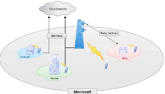
Fig 1.1 Architecture of a heterogeneous mobile network.

Fig. 2.1 Comparison of calculated and measured antenna gain.

Fig. 2.2 An example of GMM.

Fig. 2.3 Traditional grid model.

Fig. 2.4 Completely random

model.

Fig. 3.1 Mean throughput per

cell over 24 hours of measured data set from Monday to Sunday.

Fig. 3.2 Weekday and weekend

mean throughput per cell over 24 hours.

Fig. 3.3 Histogram of

throughput per cell at 5:00 and 17:45 on weekdays.

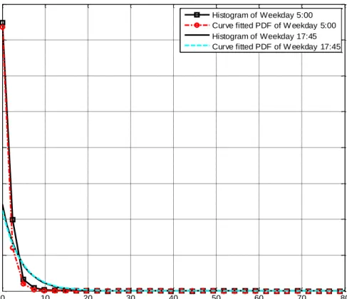
Fig. 3.4 Comparison of real-data-based histogram and curve-fitted exponential probability distribution for a weekday.

Fig.3.5 Comparison of real-data-based histogram and curve-fitted exponential probability distribution for a weekend day.

Fig. 3.6λ curve fitting results. 3 18 23 24 25 35 36 40 42 43 45

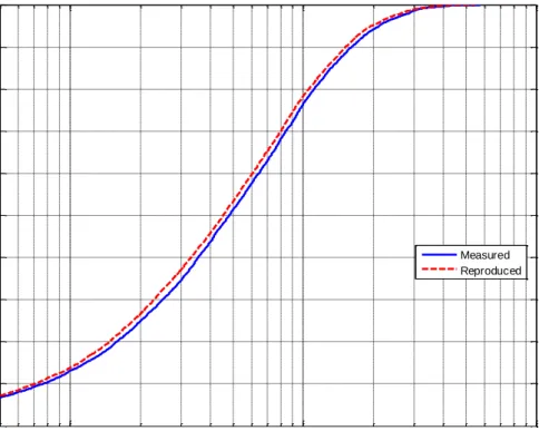
Fig. 3.7 Empirical CDFs of measured throughput per cell and reproduced throughput per cell at 17:45 on weekdays.

Fig. 3.8 Comparison of

reproduced mean throughput and measured mean

throughput.

Fig. 4.1 An instance of the problem scenario.

Fig. 4.2 The average UE throughput and minimum UE throughput versus the number of mobile small cells by FNDA.

Fig. 4.3 The average number of mobile small cells required by DOENA and by the deployment optimisation based on

maximizing sum UE throughput versus the number of HS UEs.

Fig. 4.4 The minimum UE

throughput of DOENA and maximizing sum UE throughput versus the number of HS UEs.

Fig. 4.5 The average UE throughput of DOENA and maximizing sum UE throughput versus the number of HS UEs.

Fig. 4.6 The minimum UE

throughput vs. the number of HS UEs.

Fig. 4.7 The average number of new small cells vs. the number of HS UEs.

Fig. 4.8 The SD of number of small cell UEs vs. the number of HS UEs.

Fig. 5.1 The intensity of

additional small cells in the HS 47 48 52 64 65 66 67 74 75 76

area () versus the intensity of HS UEs.

Fig. 5.2 The intensity of

additional small cells in non-HS areas (



) versus the intensity of HS UEs.

Fig. 5.3 An example of the total number of new small cells under the setting in Table 5.2.

Fig. 5.4 Average UE throughput versus the intensity of HS UEs.

Fig. 5.5 Fairness index versus the intensity of HS UEs.

Fig. 5.6 Area spectral efficiency versus the intensity of HS UEs.

Fig. 5.7 Macro-UE received interference power versus the number of additional small cells.

List of Tables

TABLE 3.1: Curve-fitting

parameters for λ.

TABLE 4.1: System Settings for FNDA and DOENA.

TABLE 5.1: Events.

TABLE 5.2: System Settings for stochastic geometry analysis. 86 87 87 93 94 95 96 46 63 80 86

Notations

𝐶- Capacity 𝐵- Bandwidth 𝑃𝑡- Transmit power 𝐴𝑃- Antenna pattern 𝑃𝐿- Path loss 𝑘- Boltzman's Constant 𝑇- Absolute temperature 𝑓_𝑐- Frequency in GHz

ℎ₁- Base station height

ℎ₂- user equipment height

ℎ𝑏𝑢𝑖𝑙𝑑𝑖𝑛𝑔- Average height of buildings

𝑊𝑠𝑡𝑟𝑒𝑒𝑡- Width of street

d-Distance

𝐴𝐻- Horizontal antenna pattern

𝐴𝑉- Vertical antenna pattern

𝜃- Azimuth angle

𝑏𝑤- Bin width

𝑇_𝑚𝑎𝑥 - Maximum values of the instantaneous throughput per cell

𝑇_𝑚𝑖𝑛 - Minimum values of the instantaneous throughput per cell

λweekday - Rate parameter for weekdays

λweekend - Rate parameter for weekend days

F

eBS

N - Number of existing base

stations

nBS

N - Number of new base stations

BS

N - Total number of base stations

nhs

N - Number of non-hot spot users

hs

N -Number of hot spot users

U

N - Total number of users

U

N - Set of users

BS

N -Set of base stations

RB

N - Set of resource blocks

i



- Throuhgput of

i

th user ,

k i j

a - Joint user allocation and resource allocation indicator

k j

P - Downlink transmit power of the jth base station

, k i j

g - Channel power gain

, k f ij g - Exponentially distributed fading gain , pl ij

g - Path loss gain

( , )x y_{i i} - Location coordinates of the

i

th user

(x y_j, _j)- Location coordinates of the jth base station

pl

 - Path loss distance exponent

0

N - Additive white Gaussian noise power

, k i j

A - Joint user association and resource allocation joint matrix

( , )x y - Coordinate vectors

th



- user throughput threshold

|H |- Feasible deployment area

B- User association matrix

, i j

b - User association indicator

C- Resource allocation matrix

, RB i j

N - Number of resource blocks allocated by the jth base station to the

i

th user

RB j

N - Number of resource blocks per user in jth base station

max nBS

N - Maximum number of new

small cells

W

- Bandwidth of a resource block

 - Non-hot spot user intensity

 - Hot spot user intensity

 - Existing small cell intensity



- Intensity of new small cells in non-hot spot area



- Intensity of new small cells in hot spot area

2 1

 - User to small cell distance correlation factor

M

R - Macrocell coverage area

H

R - Hot spot area

H

R - Hot spot area excluding the coverage area of existing small cells in the hot spot

nH

R - Non-hot spot area

AC



- Expected number of non-hot spot users in the coverage of an existing small cell base station

C



- Expected number of existing small cells in the macrocell coverage area

{ _U}

E N - Expected total number of non-hot spot users in the macrocell coverage area before hot spot occurs

ABE



- Expected number of users in a new small cell coverage in the hot spot area

AB



- Expected number of users in an existing small cell coverage that overlaps with the hot spot area

AD



- Expected number of non-hot spot users served by new small cells in non- hot spot areas

C



 - Expected number of existing small cells in non-hot spot areas

E



- Expected number of additional small cells in the hot spot area

D



- Expected number of additional small cells in non-hot spot area

{ _U}

E N - Expected total number of UEs in the macrocell coverage area with hot spot

F - Fairness index

HetNet- Heterogeneous Network

LTE- Long Term Evolution

LTE-A- Long Term Evolution

3GPP- 3rd Generation Partnership Project

MIMO- Multiple Input Multiple Output

AP- Access Points

QoS- Quality of Service

UE- User Equipment

HS- Hot Spot

OFDMA- Orthogonal Frequency

Division Multiple Access

OFDM- Orthogonal Frequency

Division Multiplexing

ISI- Inter Symbol Interference

RB- Resource Block

SINR- Signal-to-Interference-Plus-Noise Ratio

NLOS- Non-Line-of-Sight

LOS- Line-of-Sight

PDF- Probability Density Function

RMSE- Root Mean Squared Error

GMM- Gaussian Mixture Model

SPPP- Spatial Poisson Points Process

CDMA- Code-Division Multiple

Access

HSPA- High Speed Packet Access

PPP- Poisson Point Process

CDF- Cumulative Distribution

Function

FNDA- Fixed Number Deployment Algorithm

DOENA- Deployment over Existing Network Algorithm

DL- Downlink

B&B- Branch and Bound

GRG- Generalized Reduced Gradient

Content

ABSTRACT ... I ACKNOWLEDGEMENTS ... III LIST OF FIGURES ... IV LIST OF TABLES ... VI NOTATIONS ... VII CHAPTER 1 INTRODUCTION ... 1 1.1BACKGROUND ... 1 1.2MOTIVATION ... 5

1.3THESIS RESEARCH AND CONTRIBUTIONS ... 6

1.4PUBLICATIONS ... 9

CHAPTER 2 PRELIMINARIES ... 10

2.1INTRODUCTION ... 10

2.2FUNDAMENTAL CONCEPTS ... 11

2.2.1 Orthogonal Frequency Division Multiple Access ... 11

2.2.2 Small cells ... 11

2.2.3 Standards in LTE-A ... 12

2.2.4 Path loss ... 14

2.3REVIEW OF MATHEMATICAL METHODOLOGY ... 18

2.3.1 Probability Density Estimation ... 18

2.3.2 Curve Fitting ... 20

2.3.3 Gaussian Mixture Model ... 22

2.3.4 System Modelling Method ... 24

2.4RELATED WORK ... 26

2.4.1 Data Traffic Analysis ... 26

2.4.2 Small Cell Deployment in 4G HetNets... 28

2.4.3 Small Cell Deployment Based on Stochastic Geometry Analysis ... 30

CHAPTER 3 USER DATA TRAFFIC ANALYSIS ... 33

3.1INTRODUCTION ... 33

3.2MEASUREMENT DATA SET AND METHODOLOGY ... 34

3.2.1 Measurement Data Set ... 34

3.2.2 Methodology ... 36

3.3MODELLING AND RESULTS ... 38

3.4CONCLUSION ... 49

CHAPTER 4 SMALL CELL DEPLOYMENT FOR 4G HETEROGENEOUS NETWORKS ... 50

4.1ITERATIVE DEPLOYMENT ALGORITHM OF SMALL-CELLS IN HETEROGENEOUS NETWORKS ... 50

4.1.2 System Model ... 52

4.1.3 Mobile Small Cell Deployment Optimisation ... 54

4.1.4 Solving the Optimisation Problem ... 59

4.1.5 Simulation Results ... 63

4.1.6 Conclusion ... 68

4.2REDUCED-COMPLEXITY DEPLOYMENT ALGORITHM OF SMALL-CELLS IN HETEROGENEOUS NETWORKS ... 69

4.2.1 Introduction ... 69

4.2.2 System Model ... 69

4.2.3 Problem Formulation ... 71

4.2.4 Solving the Optimisation Problem ... 72

4.2.5 Simulation Results ... 73

4.2.6 Conclusion ... 77

CHAPTER 5 SMALL CELL DEPLOYMENT BASED ON STOCHASTIC GEOMETRY ANALYSIS .. 78

5.1INTRODUCTION ... 78

5.2SYSTEM MODEL ... 79

5.2.1 The Network without HS ... 81

5.2.2 The Network with HS ... 82

5.3INTENSITY OF ADDITIONAL SMALL CELLS ... 84

5.4DEPLOYMENT OF ADDITIONAL SMALL CELLS ... 89

5.6CONCLUSION ... 97

CHAPTER 6CONCLUSION AND FUTURE WORK ... 99

6.1CONCLUSION ... 99

6.2FUTURE WORK ... 101

Chapter 1

Introduction

1.1 Background

Mobile phones are much more widely used all over the world since it has been developed in 1973 [1]. Nowadays, mobile phones are not only used for voice services but also data services in last decades. The mobile communication networks as one of the greatest changes provide a brand-new life style for people. One of the most significant revolutions of mobile communications is that users can use their devices to access the Internet as long as they are in the operator’s coverage area. However, this revolution results in an exponential increase of data demands. Compared with 2014, the wireless data traffic has grown by 74 percent worldwide in 2015 [2]. This huge amount of data requirement gives operators a challenge of satisfying subscribers while

reducing power consumption and interference. From the third generation (3G) to fourth generation (4G) and fifth generation (5G), the users’ data traffic demands continue increasing. In order to reduce the pressure of macro base stations, small cells are introduced to provide higher quality signal to users.

One of the core concepts to solve the conflictions between huge data demands and limited radio resource is to increase the number of base stations in order to get a higher total capacity. Those base stations which have coverage of kilo-meter order of magnitude have been changed to hundreds of meters’ coverage which is known as macrocells. Another kind of base stations have also been developed as an additional tier of the networks which provide only dozens of

meters’ coverage which is known as small cells. Such multi-tier networks are known as heterogeneous networks (HetNets).

HetNets as an important concept in LTE-A is widely used by operators and network designers nowadays. It is anticipated that HetNets would mitigate the conflict between the rapid growth of data demand and limited radio resources by increasing the area spectral efficiency through densely deploying low-power small cells such as femtocells [3]. As a trend that mobile data demands increasing in an exponential rate and will become more and more important to people’s daily lives, the management of limited network resource is vital to HetNets. For example, a HetNet can be constructed by overlaying low-power small base stations (BSs) on top of the existing macrocell network to increase the network capacity [4].

Since Long-Term Evolution (LTE) was launched in March of 2009 [5], the 3rd Generation Partnership Project (3GPP) has been devoted to improving the performance of LTE via advanced Multiple Input Multiple Output (MIMO), carrier aggregation and HetNets, as evident from the LTE Advanced (LTE-A). HetNets use mixes of microcells, femtocells, picocells, relay BSs and other kinds of small access points cooperate with macrocells to establish flexible and low-cost networks to provide high QoS to users [3]. Fig.1.1 shows an example of architecture of a HetNet.

Small cells are low-power access points (APs) for users to access mobile networks and get services. According to the scale of coverage area and different subscribers, small cells encompass femtocell, picocell, microcell and relays.

Among these small cells, femtocell is used in home or a small business. The coverage radius of a femtocell normally is from 10 meters to 20 meters. The subscribers of femtocell made it become randomly in deployment. There are two kinds of femtocells: open access and closed access small cells. The former can serve any user belongs to its operator located in its coverage area, while the later only allows the user that has authorized to access. According to recent researches [6][7], open access femtocells have a better performance in both uplink (UL) and downlink (DL) capacity. As a result, open access femtocells will be used widely by operators in the real network environment. As a result, these kind of femtocells have capability to support users that nearby their coverage and reduce stress of macrocells loads they are located in.

Picocells are also a kind of small coverage APs, however, they have a larger coverage radius than femtocells. Normally, a picocell can provide service to a user up to 200 meters away. Picocells are often deployed in an office building, shopping mall or a stadium. The deployment of a picocell are usually participated by operators in order to control the influence of interference into an acceptable level during deploying.

Relay base stations can increase the density and coverage area of the LTE networks. Due to no separate backhaul required by a relay base station, the deployment is easier than a small cell (femto or pico). The backhaul directly

connects to the macrocell base station. Therefore, relays have slight improvement on increasing spectrum efficiency in the same area but have significant effect on increasing the QoS and extending coverage.

1.2 Motivation

Usually, operators plan HetNets are based on the expected user distribution and mobile traffic pattern which is obtained from long-term observations and big data collections. It is important to achieve both good service quality and low cost in HetNet planning and deployment. In [8], the deployment of small cells is optimised to obtain the best trade-off between user Quality of Service (QoS) and operators' costs. The dynamic small cell deployment strategy in [9] can be used to find out when and where small cells need to be deployed. However, in an existing HetNet, persistent clusters of user equipments (UEs), a.k.a., hot spots (HSs), which were not been expected in the original network planning may occur, causing extra traffic demand. Therefore, the main target of my research work is focus on the solution of additional data requirements caused by HSs.

In order to study and solve the HS problem in HetNet, it is important to understand the existing mobile network. Therefore, a data traffic analysing for existing 3G network has been undertaken first. After, three different small cell deployment strategies are developed to solve the extra data demand problem caused by HSs in 4G HetNet. These three strategies are developed in the

scenario that close to reality in 4G networks, therefore, a small cell deployment strategy that based on a theoretical analysis has been studied by using stochastic geometry analysis.

1.3 Thesis Research and Contributions

Aa a result, my research includes three aspects: 1) data traffic analysis; 2) small

cell deployment in HetNets; 3) stochastic geometry analysis and small cell deployment of HetNet. Statistical modelling of time-varying throughput per cell has been implemented in the study of 1) in order to understand the existing traffic demands for 3G network. The result is efficient and could be used in related researches. In the research of 2), the deployment strategy for 4G has been studied first with a joint optimisation of the number and locations of additional mobile small cells and the user associations of all cells carried out in order to maximizing the minimum UE throughput. Furthermore, a reduced-complexity iterative algorithm is devised to solve the joint small cell deployment optimisation problem has also been carried out. In the research of 3), small cell deployment is based on stochastic geometry analysis, a HetNet affected by a large HS and for the additional small cells that need to be deployed based on the spatial bivariate Poisson point process has been provided first and the optimal numbers of additional small cells are obtained by minimizing the difference between the numbers of macrocell users after and before the HS occurs based on the stochastic geometry analytical results. An

algorithm to maximize the average user throughput by jointly optimizing the locations of additional small cells and user associations of all cells has been developed.

The research work is presented in this thesis by the following layout:

Chapter 2 Preliminaries: This chapter introduces the background knowledge and related works of data traffic and HetNet. Concepts of HetNets architecture, femtocells, small cell deployment are introduced in this chapter. Moreover, literature reviews on the traffic load analysis, including mathematical methods to analyse a measurement data set obtained from an existing network, and small cell deployment has been presented as well.

Chapter 3 User Data Traffic Analysis: The analysis of an existing 3G network

and proposes a statistical method to predict the instantaneous throughput per cell has been presented. This is followed by a complete mathematical analysing approach to the measured data and evaluation of the result.

Chapter 4 Small Cell Deployment for 4G heterogeneous Networks: The small

cell deployment for 4G HetNet has been presented in this chapter. Firstly, a strategy to optimise the number and locations of additional mobile small cells on top of an existing HetNet to fulfil the excess traffic demand of recurring HSs that were not expected in the original HetNet planning has been proposed. Secondly, a strategy based on reduced-complexity iterative algorithm to solve the joint deployment optimisation problem has been presented. The simulation result for both strategies have been presented as well.

Chapter 5 Small Cell Deployment Based on Stochastic Geometry Analysis: An algorithm to maximize the average user throughput by jointly optimizing the locations of additional small cells and user associations of all cells has been presented that based on the stochastic geometry analysis of the HetNet with a large HS. The simulation results have been presented.

Chapter 6 Conclusion and Future Work: The summary of this research has been

1.4 Publications

 N. E, X. Chu and J. Zhang, "Small-cell deployment over existing heterogeneous networks," IET Electronics Letters, vol. 52, iss. 3, pp. 241-243, Feb 2016.

 N. E and X. Chu, "Stochastic geometry analysis and additional small cell deployment for HetNets affected by hot spots," Mobile Information Systems, Volume 2016 (2016), Article ID 9727891, pp. 1-9, Jan 2016.

 N. E, X. Chu and J. Zhang, "Mobile small-cell deployment strategy for hot spot in existing heterogeneous networks," IEEE GLOBECOM'15 WS, San Diego, CA, USA, 6-10 Dec 2015.

 N. E, X. Chu, W. Guo and J. Zhang, "User data traffic analysis for 3G cellular networks," International Conference on Communications and Networking in China (ChinaCom'13), pp. 468-472, Guilin, China, 14-16 Aug 2013.

Chapter 2

Preliminaries

2.1 Introduction

This chapter reviews concepts of 3G and 4G networks in order to support the design in the following chapters. Fundamental concepts and elements of HetNets and related techniques are listed in this chapter. Moreover, mathematical concepts and random processes are also presented, including exponential random process, density evaluation, curve-fitting, goodness of curve-fitting evaluation and mixture models. The literature review of related works is presented as well.

2.2 Fundamental Concepts

2.2.1 Orthogonal Frequency Division Multiple Access

Orthogonal Frequency Division Multiple Access (OFDMA) has been considered as the multiple access technology for mobile networks in LTE. The concept of Orthogonal Frequency Division Multiplexing (OFDM) is to divide the bandwidth into multiple orthogonal frequency sub-carriers. Therefore, the Intersymbol Interference (ISI) is completely eliminated [10]. By using time-frequency plane, the resource of OFDMA is divided into resource blocks (RBs). Each RB has 180kHz bandwidth for subcarriers. The number of subcarriers in each RB depends on the spacing of subcarriers, for example, if the subcarrier spacing is 15kHz, there are 12 subcarriers in each RB. In small cell deployment researching, RBs are considered as an essential element for resource allocating.

2.2.2 Small cells

Small cells were first introduced in 1984 [11]. The idea is to use multiple smaller cells instead of a macrocell. As mentioned in Section 2.2, a small cell needs to be self-adaptive to networks environment. For example, femtocells as a kind of small cell that has IP-based backhaul interface directly connect to core networks. The reason for small cells to be promoted is the demands of mobile

data use is increasing. In 2015, the wireless data traffic grew by 74 percent worldwide as compared with 2014, which indicates there is a large potential group of users who will require more mobile data in the future [2]. One solution of meeting this demand is increasing spatial frequency reuse by reducing the coverage of cells. Therefore, small cells are more and more popular in recent

year’s research [12].

However, the advocating of small cells brings an additional challenge. A macrocell user near a closed-access small cell AP will experience high interference [13]. There are some recent researches to solve this issue. In [14], sectorized antennas are added to femtocell APs to limit the number of interference source so as to reduce the interference in uplink. Another approach using dynamic selection of antenna patterns can also reduce the interference by reducing the power leakage outdoor [15]. Moreover, in [16], a channel switching scheme based on interference level of each available channel is provided to reduce co-channel interference to uplink.

2.2.3 Standards in LTE-A

The simulation parameters and formulas to calculate important elements in LTE-A are listed in this section. 3GPP updates new contents and revises previous

concepts frequently. It is very important to review these concepts and use appropriate methods in simulation.

The main target of optimisation is to increase the capacity of users. Shannon formula is the basic method to calculate the capacity of a radio channel:

2

C B log (1 SINR) (2.1)

where 𝐶 is capacity, 𝐵 is bandwidth. Signal-to-interference-plus-noise ratio (SINR) is used to measure the quality of wireless connections in telecommunications. It can be presented as:

Received Power SINR

Noise Interference Power



 (2.2)

where received power in this formula can be calculated by:

AP Received Power PL t P  (2.3)

where P_t is transmit power, AP is antenna pattern and PL is path loss. Interference is the sum of received power from all co-channel interferers. If we assume there are n interferers, then we have:

1 AP Interference PL n t i i i P   



(2.4)

Noise is considered as a constant value which is presented as follows:

Noise  k T B (2.5)

where k is Boltzman's Constant, 23

1.38 10 Joules / Kelvin

k    , T is absolute

temperature in Kelvin (0 C 273Kelvin).

2.2.4 Path loss

A latest path loss model can be found in [17]. This model includes non-line-of-sight (NLOS) formulas and line-of-non-line-of-sight (LOS) formulas for urban microcells and macrocells.

These models are suitable for bandwidth from 2 GHz to 6 GHz in different antenna heights. Moreover, the real world street map is also considered in this model. Therefore, simulation results will be closer to real propagation.

The microcell path loss for traditional hexagonal cell layout is presented as:

10 10

PL_LOS 22log ( ) 28 20log ( )d   f_c (2.6)

10 10

where 𝑑 is the distance in meters from user to base station and f_c is bandwidth in GHz. If taking user equipment height into consideration, this model could be presented as:

10 1 10 1

PL_LOS 40log ( ) 7.8 18log ( )d   h

10 2 10

18log ( ) 2log ( )h f_c

  (2.8)

Where d₁5000m, h₁ is base station height, h₁15m, h₂ is user equipment height, h₂1.5m.

And the macrocell path loss LOS model is represented is same as (2.6).

For NLOS model, the macrocell path loss is more complicated:

10 PL_NLOS 161.04 7.1log (W) 2 10 10 1 7.5log ( ) 24.37 3.7 log ( ) BS h h h h  _{ }       _{ }  _{ }    10 1 10 10

(43.42 3.1log ( ))(log ( ) 3) 20log ( )h d f_c

   

2 10

(3.2(log (11.75hUT)) 4.97)

where h is the average height of buildings, h20m, W is the width of street,

W 20m , h₁ in this case is 25 meters. The LOS model for macrocell in urban

environment could be changed if consider height is same with microcells.

In [18], the path loss that for general use is given by:

10

15.3 pl 10 ( )dB

PL    log d (2.10)

where pl is the path loss exponent and d is the distance. Since the generality of this path loss model, it has been implemented in this research work.

2.2.5 Antenna Gain

Antenna gain is an important element in radio propagation. Different antenna main-lobe pointing direction will have various signal strength. In [18], antenna gain has been defined. An example of using it can be found in [19].

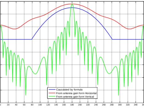
In HetNet, the horizontal antenna pattern can be presented as follows:

2 3dB A ( )_H  Amax_M min 12  , A_m   _{ }      _{   }       (2.11)

where 𝜃 is the azimuth angle relative to the main-lobe pointing direction, AmaxM 15dB, 3dB 70



 , and A_m25dB.

The vertical antenna pattern can be presented as follows:

2

3dB

A ( ) Amax min 12 etilt ,SLA

V M v      _{  }      _{   }       (2.12) Where 3dB 10 

 , SLA_v 20dB and _etilt 15 or 6 based on different simulation environment. 15 is used in 3GPP case 1 and 6 is used in 3GPP case 3. Both 3GPP case 1 and 3 have the same carrier frequency, but case 1 have a smaller inter-site distance which is 500 meters and the inter-site distance in case 3 is 1732 meters.

These formulas can be used in 3-sector antenna simulations. However, there is a set of measured antenna gain which could provide more accurate simulation result. Fig. 2.1 illustrates the difference between calculated and measured antenna gain should not be ignored.

Fig. 2.1 Comparison of calculated and measured antenna gain.

2.3 Review of Mathematical Methodology

2.3.1 Probability Density Estimation

Probability density estimation is a popular method investigating data set and its distribution. [20] introduces density estimation in detail. The primary goal of this method is to construct a density function of measured (observed) data

0 20 40 60 80 100 120 140 160 180 200 220 240 260 280 300 320 340 360 -60 -50 -40 -30 -20 -10 0 10 20 Angle () A n te n n a G a in ( d B ) Cauculated by formula From antenna gain form Horizontal From antenna gain form Vertical

samples. It is an efficient approach to obtain Probability Density Function (PDF) when studying observed data.

There are different methods to process density estimation, histograms, the naive estimator, the kernel estimator, the nearest neighbouring method, variable kernel method, orthogonal series estimators, maximum penalized likelihood estimators and so on. This research on data analysis uses histograms to estimate density distribution. Therefore, histograms method is introduced in the rest of this section.

Histogram is the oldest and famous way in density estimation. To construct a histogram, we need to first set an origin and a bin width, both of which will control the amount of smoothing inherent in the procedure and will have an effect on the obtained PDF. For example, if the observed data set is

1 2

{ ,y y ,...,y_n}, the bin width is 𝑏𝑤 and origin is 𝑜𝑟𝑖, from origin to the maximum value of this data set, there are n levels, where n is calculated by:

Maximum data value ori

n

bw



 (2.13)

For each sample that belongs to this region, it can represent 1 occurrence to the level. The total occurrence of each level illustrates the distribution of this data set. Histogram can be seen as a rough density distribution.

2.3.2 Curve Fitting

Curve fitting as a part of distribution estimation is used to construct the closest distribution function for observed data. Generally, curve fitting can be summarized to three situations of implementing which is based on the awareness of distribution function of original data [21]:

Situation 1: The distribution function is empirically known, and then the target function can be calculated directly.

Situation 2: The distribution function is empirically known but the parameter

in this function is unknown, then the parameter values need to be calculated by curve fitting methods.

Situation 3: Both distribution function and its parameters are unknown, the estimation function needs to be modelled by multiple experiments, and parameters need to be calculated.

It is known that the ultimate goal of curve fitting is to minimize the different between observed data and corresponding data. For this goal, a method known as least-squares is used. For instance, if the observed data set is { ,y y_{1 2},...,y_n}, the corresponding calculated function values are f x( )_i , the residual should be minimized as:

2

min{(y_i f x( )) }_i (2.14)

The reason to use square value is to make sure the positive and negative residuals are treated equally.

Evaluation of fitted result is essential to curve fitting procedure. There are two metrics I used to evaluate the goodness of curve fitting in my research. The first one is the square of correlation between the measured or empirical value and the predicted value, and is referred to as R-square [22]. If { ,y y1 2,...,yn} are n measured or empirical data and { ,y yˆ ˆ_{1 2},...,yˆ_n} are the n curve-fitted data, R-square can be calculated as follows:

2 1 2 1 ˆ ( ) R-Square 1 ( ) n i i i i n i i i w y y w y y      





(2.15)

where y is the mean value of { ,y y_{1 2},...,y_n}, and w_i (i1,...,n ) are the weighting factors. square takes value in the interval from 0 to 1. For a R-square value larger than 0.9, the curve fitting is usually considered to be good enough. However, it is not always the higher R-square value the better in practice. Implementation and complexity issues also need to be considered.

The second curve fitting metric is Root Mean Squared Error (RMSE) [23], which is defined as:

2 1( ˆ ) RMSE i i i n y y n   



(2.16)

where 𝑛 is the number of measurement samples. RMSE represents the total deviation of the response values from the fit to the response values. A value closer to 0 indicates that the model has a smaller random error component, and that the fit will be more useful for prediction. For a good fitting, the value of RMSE is usually less than 0.2.

2.3.3 Gaussian Mixture Model

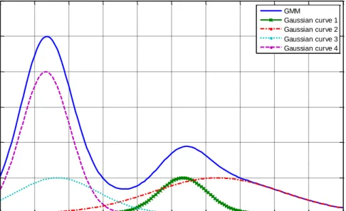
Gaussian Mixture Model (GMM) is one of the mature mixture models in statistics. Mixture models are the combination of multiple density functions to construct a multimodal density model [24]. GMM in my research is used to construct a function to fit a multi-peak curve. A GMM can be expressed as:

2 1 GMM

( )

i i x b n c i i a e    



(2.17)

where 𝑎𝑖 is the amplitude, 𝑏𝑖 is known as the centroid location, 𝑐𝑖 relates to the peak width, and n represents the number of peaks of the data series. For example, Fig. 2.2 shows a four-peak GMM and its component Gaussian functions.

Fig. 2.2 An example of GMM.

The reason GMM is used in my research is because the real measured data is multi-peak and multi-density. GMM can construct an appropriate model to fit it. Moreover, the characteristics of a GMM are controlled by the parameters of each component Gaussian function, which is easy in operation.

0 3 6 9 12 15 18 21 24 27 30 0 1 2 3 4 5 6 GMM Gaussian curve 1 Gaussian curve 2 Gaussian curve 3 Gaussian curve 4

2.3.4 System Modelling Method

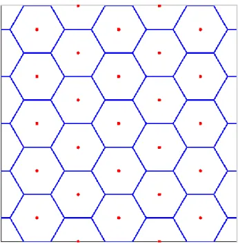
There are two types of system models that can be used in HetNet analysis and simulation. One is the traditional grid model, which is considered as a well-planned network environment. The other one is a completely random model. Generally, these two types of system model can be used in most simulation conditions. Fig 2.3 is an example the graph of traditional grid model. A widely used model of this is only drawing three layers of cells which contain nineteen cells.

Traditional grid model is very popular in simulation, where the femtocell APs are distributed randomly in each macrocell. As the location of each macrocell base station is fixed, interference from macrocells in this model is calculated relatively simple. Traditional grid model provides an ordered environment which can be used in preliminary scheme study. However, traditional grid model is significantly distinct from real network, especially in urban-areas. Due to competition among multiple operators and complicated environment effect, the deployment of base stations is anomalous. As a result, it is insufficient only applying traditional grid model in simulation.

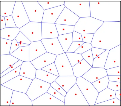
Fig 2.4 shows an example of completely random model. Completely random model is acknowledged closer to real network. The location of each base station follows Spatial Poisson Points Process (SPPP), special cases such as overlaid macrocell base stations will be illustrated in this model. Due to the simulation result in this model will be closer to real world, unexpected issues have a higher possibility to be found in advance before implement.

2.4 Related work

2.4.1 Data Traffic Analysis

Data traffic analysis for cellular networks is an essential method to explore the limitation and issues that may occur. Several recent papers have reported data traffic analysis for different purposes. In [25] and [26], data traffic analysis was used to develop dynamic spectrum access approaches by analysing three weeks’

voice traffic in an urban area in northern California. These two papers discuss call durations and exponential call arrival model. In [27], the authors modelled each cell as an independent M/G/∞ queue, with the number of users in each cell modelled as an independent Poisson random process, in order to predict the traffic capacity of code-division multiple access (CDMA) networks. User-behaviour measurements of a High Speed Packet Access (HSPA) network were presented in [28], where measurements made at network, cell and user-session

levels were studied separately. The analysis of the network-level data was based on the measured throughputs of only one day. For cell-level data analysis, the empirical cumulative distribution function (CDF) of the throughput per cell was obtained by using Poisson fitting. Moreover, the mean throughput per user-session was modelled as a log-normal distributed random process. In [29], large-scale Third Generation (3G) network data traffic was studied based on CDF of data traffic measurements to provide insights on traffic load, but there lacked an analysis on cell level throughput. Large-scale cellular data traffic measurements are difficult to obtain, as a result, little effort has been made in the literatures to develop statistical models based on real cellular network data to predict user data traffic distributions in time and in space. In [30] the user data traffic analysis is based on a nationwide 3G network data. Spatial correlation has been characterized by using 10 minutes and 1 hour granularities in order to using cross-correlation method to investigate the spatial correlation. Another research based on the location and traffic records data from radio access network and core network in a 3G data network of United States has been carried out in [31]. The analysis shows that the data traffic is significant different for the BS clusters in different geographical regions.

2.4.2 Small Cell Deployment in 4G HetNets

It is known that a HetNet is usually planned based on the expected user distribution and mobile traffic pattern obtained from long-term observations and statistical data. It is important to achieve both good service quality and low cost in HetNet planning and deployment. In [7], the deployment of small cells is optimised to obtain the best trade-off between user QoS and operators' costs. The dynamic small cell deployment strategy in [8] can be used to find out when and where small cells need to be deployed. Another study in 2015 presents a small cell deployment scheme that considers user location varying [32]. An iterative location deployment updating algorithm has been developed to optimise the deployment and resource allocation. Also, in [33], the small cell deployment is optimised by an algorithm based on weighted k-mean mechanism. By a given number of small cells to be deployed, k-means algorithm is used to optimise the locations of the small cells based on the different data demands. The study of small cell deployment is still popular, [34] [35] [36] [37] are recent studies for small cell deployment in different scenarios. In [34], a two-tier network with micro and pico tier has been analysed by the authors in order to optimise the energy efficiency problem. A small cell deployment scheme has been developed in [35] to solve the problem for cells are placed in biased manner. The work in [36] studies the small cell deployment problem by maximizing service time. The authors of [37] use joint optimisation to solve the deployment and small cell management together by maximizing the utility of

users and network operators. The localisation system for two-tier network planning is discussed in [38].

Once a HetNet has been deployed, its radio resources need to be reused among neighbouring cells and the network capacity is limited by inter-cell interference. In [39], interference management is achieved by controlling the number of RBs that can be used by small cells. In [40], the resource allocation and user association strategies are investigated for the orthogonal deployment, co-channel deployment and partially shared deployment of small cells.

When unexpected HS occurs in an existing HetNet causes mobile traffic demand goes beyond the network capacity, additional small cells may need to be deployed on top of the existing HetNet. In this case, the strategies in [7] [8] [41] and the structured deployment strategy in [42] would require the redesign of the overall HetNet to achieve the optimised deployment. In [43], the optimised deployment locations of new small cells are selected from a set of candidate locations, which need to be obtained before the optimisation process, making it less effective for unexpected but reoccurring HSs. Moreover, without constraint of minimum UE throughput, maximizing the sum throughput or average UE throughput [44] might still leave some UEs with dissatisfied QoS.

2.4.3 Small Cell Deployment Based on Stochastic Geometry

Analysis

Small cell deployment in HetNets has been considered as an efficient solution to the rapid growth of mobile data demand under limited radio resources. It is anticipated that deploying low-power small cells will increase the area spectral efficiency [3]. In a HetNet, some small cells are deployed by the users, with their locations uncontrollable by the operators. Moreover, once a HetNet has been deployed, persistent HSs of UEs that were not expected in the original network planning may occur, causing extra traffic demand. As the mobile traffic demand goes beyond the network capacity, the QoS of UEs in the HetNet will be affected. In this case, deploying additional small cells on top of the existing HetNet by the operators would become necessary.

Considering cost effectiveness for network operators, it is desirable to optimise the number and locations of additional small cells to be deployed without changing the existing HetNet infrastructure. This relies on a thorough analysis of the HetNet. Stochastic geometry and the theory of random geometric graphs have been used in the analysis and design of wireless networks [45]. In [46], the stochastic geometry is used to analyse the outage probability for multi-cell cooperation. Also, stochastic geometry is used to analyse the coverage probability of cellular system [47] [48] [49]. Stochastic geometry has also been used in deployment strategies, for instance, a recent research in [50] proposes a deployment strategy by applying tools from stochastic geometry in a

multi-tier HetNet. The optimised deployment is obtained by minimizing the area power consumption. Another deployment strategy that considers energy efficiency based on stochastic geometry tools is carried out in [51]. The relation between the average coverage probability and deployment strategy is derived by the stochastic geometry tools.

Poisson point process (PPP) as a popular model tool in HetNet is applied in the research of this work. The inter-nodal distances were modelled using a spatial bivariate PPP in [52]. A recent research on HetNet use independent PPP to model the locations of BSs [53]. Moreover, in [54], the locations of BSs and UEs are modelled by two independent PPPs in HetNet. In [55], Spatial Poisson Point Process (SPPP) is also considered to be used in the urban and suburban regions in HetNets. An isotropic SPPP are introduced in a recent research [56] is also used in two-tier femtocell networks.

Although HS mitigation has been studied for wireless sensor networks [57], most existing works on small cell deployment strategies focused on optimizing the deployment of small cells on top of a conventional macrocell network or the deployment of a whole new HetNet from scratch [7] [8] [41] [42] [44]. There is a lack of strategies for deploying additional small cells on top of an existing HetNet in response to extra traffic demand from HSs that were not expected in the original network planning. It is especially challenging to optimise both the number and the locations of additional small cells to be deployed. Small cell

deployment for different scenarios are also popular, for instance, a study of dense small cell deployment is introduced in [58].

Chapter 3

User Data Traffic Analysis

3.1 Introduction

In this chapter, an analysis of 3G network user data traffic is presented. It is important to understand the operation of an existing cellular network. Investigating cellular user data traffic changes over time in an existing network is an efficient method to understanding the characteristics of cellular networks. In this work, a statistical modelling of time-varying throughput per cell and the distribution of instantaneous throughput per cell over different cells based on throughput measurements from a real-world large-scale urban cellular network is provided.

3.2.1 Measurement Data Set

The data set is collected from 1,668 NodeBs of a 3G cellular network located in central London, United Kingdom. A series of real-time DL throughput was recorded every 15 minutes at each of these NodeBs over exactly one week (168 hours). The data traffic measurements are given in terms of DL throughput per cell in Mbit/s. Over a million data samples have been recorded in this period of time as a result. The information of each data sample includes the identity of cell, time of measurement and DL throughput value which represents the instantaneous throughput per cell.

However, the measurement data set does not include any information about the number of active users in each cell, user session duration, or traffic type (e.g., voice or data). Consequently, the research focuses on data analysis at the network level rather than the cell level, to provide insights for macroscopic management of an existing 3G network.

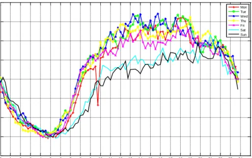
Fig. 3.1 Mean throughput per cell over 24 hours of measured data set from Monday to Sunday.

It is easily visible that the mean throughput per cell on Saturday and Sunday is significantly different from Monday to Friday. According to the observed difference in user traffic demands, the measurement data set has been divided into two groups, weekdays and weekends, respectively, for the subsequent statistical analysis. One of the reasons to separate the data set is people activities in weekdays and weekends have their different manifestations on data demands. And the second reason is that taking the sensitivity of the curve-fitting result into consideration, modelling each day of a week could reduce the generality of the random process. Moreover, the possibility of outliers existing in process of recording the data set cannot be excluded, increasing the number of samples in given time of a weekday or a weekend day can reduce the effect these outliers to the result. In consequence, Fig. 3.2 shows the weekday and weekend mean throughput per cell over 24 hours.

0 1 2 3 4 5 6 7 8 9 10 11 12 13 14 15 16 17 18 19 20 21 22 23 24 0 1 2 3 4 5 6 7 day time M e a n T h ro u p u t p e r C e ll ( M b it /s ) Wed Thu Fri Sat Sun

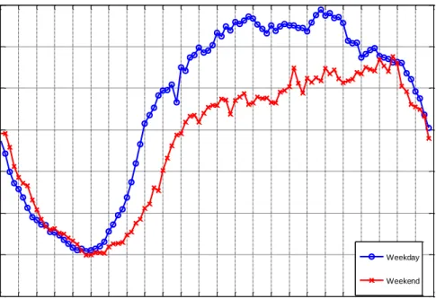
Fig. 3.2 Weekday and weekend mean throughput per cell over 24 hours.

3.2.2 Methodology

The methodology of user data analysis can be divided into following aspects:

I. Density estimation for PDF of the instantaneous throughput of a cell at a

given time in a given day.

II. Curve-fitting from PDF and estimate the parameter of fitted density

function.

III. Get the distribution over 24 hours.

IV. Curve-fitting the parameters over time and get appropriate function using

time as variable.

V. Evaluate the result by reproducing the instantaneous throughput per cell

using the fitted distribution model.

0 1 2 3 4 5 6 7 8 9 10 11 12 13 14 15 16 17 18 19 20 21 22 23 24 0 1 2 3 4 5 6 7 Time (o'clock) M e a n T h ro u p u t p e r C e ll (M b it /s ) Weekday Weekend

method in this process as mentioned in Chapter 2, Section 2.4.1. The origin for histogram is set as 0, and the bin width is present as follows:

bin width= (Tmax-Tmin)

(Tmax-Tmean)×_TdayTmean mean

(3.1)

where 𝑇_𝑚𝑎𝑥 and 𝑇_𝑚𝑖𝑛 are the maximum and minimum values of the instantaneous throughput per cell at a given time instant among all NodeBs from Monday to Friday (for a weekday) or over Saturday and Sunday (for a weekend day), 𝑇_{𝑚𝑒𝑎𝑛} is the mean value of all NodeBs’ instantaneous throughput at a given time instant average from Monday to Friday (for a weekday) or over Saturday and Sunday (for a weekend day), and 𝑇𝑑𝑎𝑦 𝑚𝑒𝑎𝑛 is the mean throughput per cell over all sampling time instants from Monday to Friday (for a weekday) or over Saturday and Sunday (for a weekend day) and among all NodeBs.

A varying bin width is used in this density estimation for different time instants of a weekday or a weekend day is because the maximum values of instantaneous throughput per cell over all the NodeBs are significantly different for different time instants of a weekday or a weekend day. For example, the highest mean throughput among all given time is blow 7 Mbit/s, and the highest instantaneous throughput of a single NodeB can be over 300 Mbit/s. For a curve, mean value, somehow, represents the importance of each sample in curve-fitting. Therefore, a weight needs to be added to each sample to maintain the curve-fitting process to limit deviation between the results and measured data on an acceptable level. The bin width given in the function adapts to the maximum instantaneous throughput of the corresponding sampling time instant of a weekday or a weekend day, so that the influence of the maximum instantaneous throughput value to the PDF estimation process can be reduced.

carried out. In this process, the main method of curve fitting is least-squared. This method involves both linear and non-linear curve fitting models. The curve fitting procedure of each given time is evaluated by the two metrics mentioned in Chapter 2, Section 2.4.2, R-square and RMSE.

The PDF approximately follows the exponential distribution, which only have one parameter. This represents each given time will have its own parameter. As a result, these parameters are addressed into a time-varying model which is a multi-peak curve. In order to get a function using time as variable, GMM is applied to construct the time-varying distribution function for parameters for the fitted PDF of instantaneous throughput per cell.

The evaluation of fitted result is executing by comparing of reproduced and measured throughput per cell in cell-level Cumulative Distribution Function (CDF) and mean throughput over 24 hours for a weekday or a weekend day, respectively.

3.3 Modelling and Results

The first step is to investigate how cellular DL throughputs change over time, which is illustrated in Fig. 3.2. The mean throughputs per cell versus different time instants over 24 hours for weekday and weekend are showed separately. For any given time-instant, the weekday mean throughput per cell was obtained by averaging the throughputs measured at that time over all the 1,668 NodeBs and over 5 workdays; while the weekend mean throughput per cell was obtained by averaging the throughputs at that time instant over all the 1,668 NodeBs and over Saturday and Sunday.

reveals. For weekdays, the mean throughput per cell has the minimum value at 5:00 and hits the maximum at around 17:45. For weekends, the minimum mean throughput per cell occurs at 5:00 while the maximum occurs at 22:00. Both weekday and weekend have the lowest mean throughput per cell of around 1 Mbit/s, but the maximum mean throughput per cell is nearly 7 Mbit/s for weekdays as compared with 5.7 Mbit/s for weekends. Moreover, from 6:00 to 21:00 the mean throughput per cell in a weekday is much higher than that in weekends, which is in accordance with the office hours from Monday to Friday.

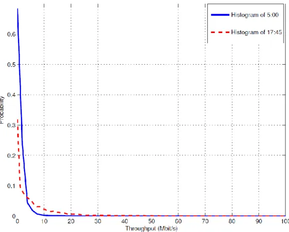
According to the observed difference in user traffic demands between weekdays and weekends, the measurement data set has been divided into two parts for weekdays and weekends, respectively. In addition to the time-varying nature of cellular traffic load, it is anticipated that different cells would have different traffic loads at any given time. Fig. 3.3 shows the histograms of throughput per cell at 5:00 and 17:45 on a weekday, which were obtained based on the throughput measurements of all the 1,668 NodeBs at these two time-instance from Monday to Friday.

Fig. 3.3 Histogram of throughput per cell at 5:00 and 17:45 on weekdays.

As mentioned in Section 3.2.2 the probability distribution of throughput per cell at the considered time instants approximately follows the exponential distribution. The PDF of an exponential distribution is given by:

𝑓(𝑥) = 𝜆𝑒−𝜆𝑥, 𝑥 ≥ 0. (3.2)

where λ is called the rate parameter for exponential distribution.

In order to find the PDF of exponential distribution that closely matches the probability distribution of throughput per cell at a given time, curve fitting is performed for the histogram of instantaneous throughput per cell using the least-squares method where the values of λ are calculated.

recorded at 1,668 NodeBs every 15 minutes over one whole week, all the available throughput samples have been group into two sub-sets: one for the five weekdays, and the other for the two weekend days. There are 96 sampling time instants each day. We assume that the probability distribution of throughput per cell at any time of a day is the same for each weekday (i.e., Monday to Friday), and is the same for each weekend day (i.e., Saturday and Sunday), respectively. We generate histograms and then perform curve fitting to get 96 PDFs for the 96 sampling time instants of a weekday based on the throughput samples of the five weekdays, and do the same for the 96 sampling time instants of a weekend day based on the throughput samples of Saturday and Sunday. R-square and RMSE have been evaluated for all the 192 PDFs obtained from curve fitting, where each obtained PDF has a R-square value higher than 0.9 and a value of RMSE lower than 0.2. Fig.3.4 compares the real-data-based histogram and the curve-fitting obtained exponential probability distribution of throughput per cell for 5:00 and 17:45 of a weekday, where

Fig. 3.4 Comparison of real-data-based histogram and curve-fitted exponential probability distribution for a weekday.

Similar comparisons are presented in Fig.3.5 for 5:00 and 22:00 of a weekend day, where λ= 0.8673 for 5:00, while λ= 0.1951 for 22:00. From both figures we can see that the curve-fitting obtained exponential distribution closely matches the corresponding real-data histogram of throughput per cell.

0 10 20 30 40 50 60 70 80 0 0.1 0.2 0.3 0.4 0.5 0.6 0.7

Throughput per cell (Mbit/s)

P ro b a b il it y Histogram of Weekday 5:00 Curve fitted PDF of W eekday 5:00 Histogram of Weekday 17:45 Curve fitted PDF of W eekday 17:45

Fig.3.5 Comparison of real-data-based histogram and curve-fitted exponential probability distribution for a weekend day.

The curve-fitting results show that the throughput per cell follows a different exponential distribution (with different values of λ) for each different time of a day (weekday or weekend). Since the 3G network traffic data set contains instantaneous throughputs measured at each cell every 15 minutes over a whole week, the process of curve-fitting based on the data set can produce 96 exponential PDFs for the 96 sampling time instants of a weekday and another 96 exponential PDFs for the 96 sampling time instants of a weekend day. As a result, the statistical results need to be presented in 192 exponential PDFs, i.e., 192 different values of λ. This is not convenient to regenerate cellular throughput data, e.g., for system-level simulations that require time-varying instantaneous throughputs at all cells of a network. In order to facilitate the use of our curve-fitting results, the function that can model how λ varies with time

0 10 20 30 40 50 60 70 0 0.1 0.2 0.3 0.4 0.5 0.6

Throughput per cell (Mbit/s)

P ro b a b il it y Curve-fitted PDF of W eekend 5:00 Histogram of Weekend 22:00 Curve-fitted PDF of W eekend 22:00

can be easily generated for any given time of a weekday or a weekend day.

In Fig.3.6, the previously obtained λ is plotted as a function of time for both weekday and weekend. According to the λ curves plotted in Fig.3.6, GMM in (2.18) is used to model the time varying behaviour of λ:

λ = ∑ 𝑎_𝑖×𝑒−( 𝑥−𝑏𝑖 𝑐𝑖 ) 2 𝑛 𝑖=1 (3.3)

for which the variable 𝑥 in (3.3) represents time and can be any time instant in the 24 hours of a day. The results of curve fitting for λ on weekday and weekend are also included in Fig. 3.6, Table I presents the fitted values of 𝑎_𝑖, 𝑏_𝑖, 𝑐_𝑖 and n. The evaluation of this curve-fitting is similar with previous PDF curve-fitting process. R-squares and RMSE values are calculated to evaluate the curve fitting for λ. For both weekday and weekend, R-square values are larger than 0.99 and RMSE values are less than 0.1. As mentioned in Chapter 2, Section 2.4.2, this indicates that the fitted results are extremely accurate.

(a) λ curve fitting result for a weekday

(b) λ curve fitting result for a weekend day Fig. 3.6 λ curve fitting results.

0 1 2 3 4 5 6 7 8 9 10 11 12 13 14 15 16 17 18 19 20 21 22 23 24 0 0.2 0.4 0.6 0.8 1 Time (o'clock) V a lu e   GMM fitted 0 1 2 3 4 5 6 7 8 9 10 11 12 13 14 15 16 17 18 19 20 21 22 23 24 0 0.1 0.2 0.3 0.4 0.5 0.6 0.7 0.8 0.9 1 Time (o'clock) V a lu e   GMM fitted

In order to evaluate the usefulness of our statistical models for cellular network simulations, the DL throughputs of 1,668 cells has been reproduced by using the statistical models and compare them with the DL throughput measurements. The evaluation is separated in two parts, CDF comparison and mean throughput over 24 hours’ comparison.

The comparison between the empirical CDFs of measured throughput per cell and statistical-model reproduced throughput per cell at 17:45 on weekdays is depicted in Fig.3.7. It can be seen that the constructed statistical model slightly underestimates (but still closely matches) the measured throughput pre cell.

Fig. 3.7 Empirical CDFs of measured throughput per cell and reproduced throughput per cell at 17:45 on weekdays.

The comparison of mean throughput between reproduced throughput and measured throughput over 24 hours in a weekday and a weekend day are illustrated in Fig.3.8 (a) and Fig.3.8 (b), respectively. From the result, we can see that although there are gaps between the mean throughputs per cell of reproduced data and that of the measured data, the model-reproduced data traffic catches the time-varying trend and spatial distribution of the measured data traffic. Hence, the statistical models could be used in simulations of urban-area large-scale cellular networks.

103 104 105 0 0.1 0.2 0.3 0.4 0.5 0.6 0.7 0.8 0.9

Throughput per cell (Kbit/s)

E m p ir ica l C D F Measured Reproduced

(a) Comparison of measured and reproduced mean throughputs per cell of a weekday.

(b) Comparison of measured and reproduced mean throughputs per cell of a weekend day. Fig. 3.8: Comparison of reproduced mean throughput and measured mean throughput.

0 1 2 3 4 5 6 7 8 9 10 11 12 13 14 15 16 17 18 19 20 21 22 23 24 0 1 2 3 4 5 6 Time (o'clock) M e a n T h ro u g h p u t p e r C e ll ( M b it /s) Generated Measured 0 1 2 3 4 5 6 7 8 9 10 11 12 13 14 15 16 17 18 19 20 21 22 23 24 0 1 2 3 4 5 6 Time (o'clock) M e a n T h ro u g h p u t p e r C e ll ( M b it /s) Generated Measured