A HUMAN DRIVER MODEL FOR AUTONOMOUS LANE CHANGING IN HIGHWAYS: PREDICTIVE FUZZY MARKOV GAME DRIVING STRATEGY
A Dissertation by
SERDAR COSKUN
Submitted to the Office of Graduate and Professional Studies of Texas A&M University
in partial fulfillment of the requirements for the degree of DOCTOR OF PHILOSOPHY
Chair of Committee, Reza Langari Committee Members, Pilwon Hur
Swaroop Darbha
Shankar P. Bhattacharyya Head of Department, Andreas A. Polycarpou
December 2018
Major Subject: Mechanical Engineering
ABSTRACT
This study presents an integrated hybrid solution to mandatory lane changing problem to deal with accident avoidance by choosing a safe gap in highway driving. To manage this, a comprehensive treatment to a lane change active safety design is proposed from dynamics, control, and decision making aspects.
My effort first goes on driver behaviors and relating human reasoning of threat in driving for modeling a decision making strategy. It consists of two main parts; threat as-sessment in traffic participants,(T V s)states, and decision making. The first part utilizes an complementary threat assessment ofT V s, relative to the subject vehicle,SV, by eval-uating the traffic quantities. Then I propose a decision strategy, which is based on Markov decision processes (MDPs) that abstract the traffic environment with a set of actions, tran-sition probabilities, and corresponding utility rewards. Further, the interactions of theT V s are employed to set up a real traffic condition by using game theoretic approach. The ques-tion to be addressed here is that how an autonomous vehicle optimally interacts with the surrounding vehicles for a gap selection so that more effective performance of the overall traffic flow can be captured. Finding a safe gap is performed via maximizing an objective function among several candidates. A future prediction engine thus is embedded in the design, which simulates and seeks for a solution such that the objective function is maxi-mized at each time step over a horizon. The combined system therefore forms a predictive fuzzy Markov game (FMG) since it is to perform a predictiveinteractivedriving strategy to avoid accidents for a given traffic environment. I show the effect of interactions in de-cision making process by proposing both cooperative and non-cooperative Markov game strategies for enhanced traffic safety and mobility. This level is called the higher level controller. I further focus on generating a driver controller to complement the automated
car’s safe driving. To compute this, model predictive controller (MPC) is utilized. The success of the combined decision process and trajectory generation is evaluated with a set of different traffic scenarios in dSPACE virtual driving environment.
Next, I consider designing an active front steering (AFS) and direct yaw moment con-trol (DYC) as the lower level controller that performs a lane change task with enhanced handling performance in the presence of varying front and rear cornering stiffnesses. I pro-pose a new control scheme that integrates active front steering and the direct yaw moment control to enhance the vehicle handling and stability. I obtain the nonlinear tire forces with Pacejka model, and convert the nonlinear tire stiffnesses to parameter space to design a linear parameter varying controller (LPV) for combined AFS and DYC to perform a commanded lane change task. Further, the nonlinear vehicle lateral dynamics is modeled with Takagi-Sugeno (T-S) framework. A state-feedback fuzzyH∞ controller is designed for both stability and tracking reference. Simulation study confirms that the performance of the proposed methods is quite satisfactory.
ACKNOWLEDGMENTS
Last four years of my Ph.D. study at the Texas A&M University has been a great experience and success that I would have never thought to become true. First of all, I would like to thank my advisor, Dr. Langari, for his support and always driving me to the right direction in research. I have developed discipline and skills to overcome any of the challenges I have encountered along the way. This work would not have been possible without the guidance of him.
I would like to thank the committee members for their suggestions and criticisms that eventually better increased the quality of this work. I would also like to thank to my colleagues for useful discussions and always encouraging me to create something better in research.
Special thank goes to the Turkish Ministry of National Education for their continuous financial support throughout my graduate studies in the United States of America.
Most importantly, I would like to express my sincere feelings to my family. They have been always supportive since I made the decision of pursuing my graduate degrees abroad. Without them, I would never have been able to become the person I am today.
CONTRIBUTORS AND FUNDING SOURCES
Contributors
This work was supervised by a dissertation committee consisting of Professor Reza Langari, Pilwon Hur, and Swaroop Darbha of the Department of Mechanical Engineer-ing and Professor Shankar Bhattacharyya of the Department of Electrical and Computer Engineering.
All work for the dissertation was completed by the student, under the advisement of Reza Langari of the Department of Mechanical Engineering.
Funding Sources
This graduate study was supported by the Turkish Ministry of National Education with the Law number 1416, under the grant name Graduate Studies Scholarship in the United States of America.
NOMENCLATURE
Driver model Overall model of autonomous driving
Hybrid system Combination of discrete and continuous system dynamics
FMDP Fuzzy Markov decision process
FMG Fuzzy Markov game
SV Subject car
Lead car The followed car by the subject car
TVs Traffic vehicles
Kinematic model Point-mass vehicle model
Gap Longitudinal space between two traveling vehicles
IDM Intelligent driver model
QP Quadratic programming
Convex set A set wherein any two points connect without leaving the set
Reach Reachable states of a dynamic system
Trajectory A line connects a vehicle’s initial and final states in a planar plane
RP Relative position
RV Relative velocity
CV Cruising velocity
MPC Model predictive control
DYC Direct yaw moment control
LMIs Linear matrix inequalities
Reference Model Linearized model of nonlinear vehicle model
BRL Bounded real lemma
LPV Linear parameter varying
T-S Takagi-Sugeno
Symbols
k Discrete Time Index
∆(k),ts Sampling Time
x Longitudinal Driving Direction on a Road Frame
y Lateral Driving Direction on Road Frame
q Threat Between SV and a TV
a Action of SV and TVs
ux Acceleration of SV and TVs in Longitudinal Direction
uy Acceleration of SV and TVs in Lateral Direction
lc Veering
N Prediction Horizon
L Transition Probabilities
%1 Weight Term on Gap
%2 Weight Term on Distance to Lead Vehicle
Ψ Gap Length Between TVs
τ Time to Reach to a Selected Gap
π Remaining Gap Length from the Lead Vehicle
m Mass of Car
Wc Width of Car
vx Longitudinal Velocity
vy Lateral Velocity
yref Reference Lane Target
T Headway Time
K Gain of Heuristic IDM
ddc Decision Evaluation Distance
WL Lane Width
Qvx Running Cost Weight on Reference Longitudinal
Velocity
Qy Running Cost Weight on Lateral Lateral
Qvy Running Cost Weight on Lateral Velocity
Rux Weight on Longitudinal Acceleration
Ruy Weight on Lateral Acceleration
˙
ψ Yaw Rate
β Vehicle Side Slip Angle
Fyf, Fcf Lateral Front Tire Force Fyr, Fcr Lateral Rear Tire Force
Flf Longitudinal Front Tire Force
Flr Longitudinal Rear Tire Force
Cf Front Tire Cornering Stiffness
Cr Rear Tire Cornering Stiffness
αf Front Tire Slip Angle
δf Front Steering Angle
δ? Corrective Steering Angle
M Yaw Moment
lf Front Tire Distance from Center of Gravity
lr Rear Tire Distance from Center of Gravity
tf Front Axle Length
tr Rear Axle Length
J Moment of Inertia
Yw Lateral Wind Gust Disturbance
L Look Ahead Distance
s Side Slip Ratio
µ Tire-Road Friction Coefficient
Fz Tire Vertical Force
J Multi-Objective Quadratic Cost Function
H∞ H∞Optimal Control
L2 H∞Norm for Nonlinear Systems
kyk2 L2 Norm of a Signaly
γ H∞Performance Index
TABLE OF CONTENTS
Page
ABSTRACT . . . ii
ACKNOWLEDGMENTS . . . iv
CONTRIBUTORS AND FUNDING SOURCES . . . v
NOMENCLATURE . . . vi
TABLE OF CONTENTS . . . x
LIST OF FIGURES . . . xiii
LIST OF TABLES . . . xvii
1. INTRODUCTION AND LITERATURE REVIEW . . . 1
1.1 Background . . . 1
1.2 Objectives . . . 3
1.3 Background and Literature Review . . . 5
1.3.1 Driver Decision Models (Higher Level Controller) . . . 5
1.3.2 Markov Decision Process (MDPs) . . . 17
1.3.2.1 MDPs in autonomous driving . . . 18
1.3.3 Game Theory . . . 20
1.3.3.1 Game Theory in autonomous driving . . . 20
1.3.4 Trajectory Planning for Autonomous Vehicles . . . 22
1.3.5 Longitudinal Vehicle Control . . . 24
1.3.6 Lateral Vehicle Control . . . 26
1.3.7 H∞Based Linear Parameter Varying (LPV) Control . . . 27
1.3.8 LPV Control in Automative Research . . . 28
1.3.9 Takagi-SugenoH∞Control Strategy . . . 33
1.3.10 Driving Safety . . . 34
1.3.11 Contribution of the Dissertation . . . 36
2. DECISION MODEL . . . 39
2.1 Instantaneous Threat Estimation ofT V sUsing Fuzzy Logic . . . 40
2.1.2 Fuzzy Inference . . . 46
2.1.3 Simulation . . . 48
2.1.3.1 Car following model . . . 48
2.1.3.2 Simulation set-up . . . 49
2.2 Prediction . . . 52
2.3 Markov Decision Process . . . 55
2.3.1 Markov Chain . . . 55
2.3.2 MDP Modeling in Autonomous Driving . . . 57
2.3.3 MDP for Gap Selection . . . 58
2.3.4 Bellman’s Equation and System Algorithm . . . 64
2.4 Markov Game . . . 66
2.4.1 Nash Equilibrium for Bimatrix Games [110] . . . 68
2.4.2 Markov Game for Gap Selection . . . 69
2.4.3 Bellman Equation for Markov Game . . . 77
2.5 Optimal Control Problem . . . 80
2.5.1 Model Predictive Control . . . 82
2.6 Trajectory Generation . . . 83
2.7 dSPACE Simulation Results . . . 86
2.8 Conclusion . . . 91
3. VEHICLE LATERAL DYNAMICS AND CONTROL . . . 94
3.1 Linear Bicycle Model . . . 95
3.1.1 H∞Steering Control Design . . . 99
3.1.1.1 Performance weight selection . . . 100
3.1.1.2 Human driver model control for lane change maneuver . 104 3.1.2 Simulation Results . . . 105
3.2 Nonlinear Vehicle Model . . . 109
3.2.1 Simplified Model . . . 111
3.2.2 Tire Model . . . 112
3.2.3 Control Design Procedure . . . 113
3.2.3.1 Performance weight selection . . . 115
3.2.3.2 LPV/H∞controller design . . . 115
3.2.4 Simulation Results . . . 120
3.3 Takagi-Sugeno Modeling for Vehicle Lateral Dynamics . . . 126
3.3.1 T-S Fuzzy modeling . . . 128
3.3.2 Controller Design . . . 132
3.3.3 FuzzyH∞Controller Synthesis . . . 134
3.3.4 Simulation Results . . . 136
3.4 Conclusion . . . 140
4. CONCLUSION . . . 143
LIST OF FIGURES
FIGURE Page
1.1 Driver model of an autonomous vehicle . . . 4
1.2 Schematic diagram of the proposed driver model . . . 5
1.3 Kondo’s driver model . . . 8
1.4 Transfer function of driver model . . . 9
1.5 A schematic process of a human like decision making. Human brain col-lects the information from environment and processes based on a subjec-tive reasoning process and executes an output according to the current state of cognition. . . 15
1.6 Illustration of an MDP with two states and two actions. The transition probabilities and rewards are given by tuples (p, R) . . . 18
1.7 An example of a path . . . 23
1.8 A car following model in highway driving. The subject car is in the middle, and the front vehicle is the lead car. The subject vehicle reacts to the change in the speed of the lead car. The rear car also reacts to the speed change of the subject car. . . 25
1.9 Type of suspension systems . . . 30
1.10 An emergency situation in traffic. The driver is not able to respond to the situation sufficiently. The proposed system take over the control of the vehicle and executes a humanlike decision to avoid the object as well as not crashing the other cars. . . 35
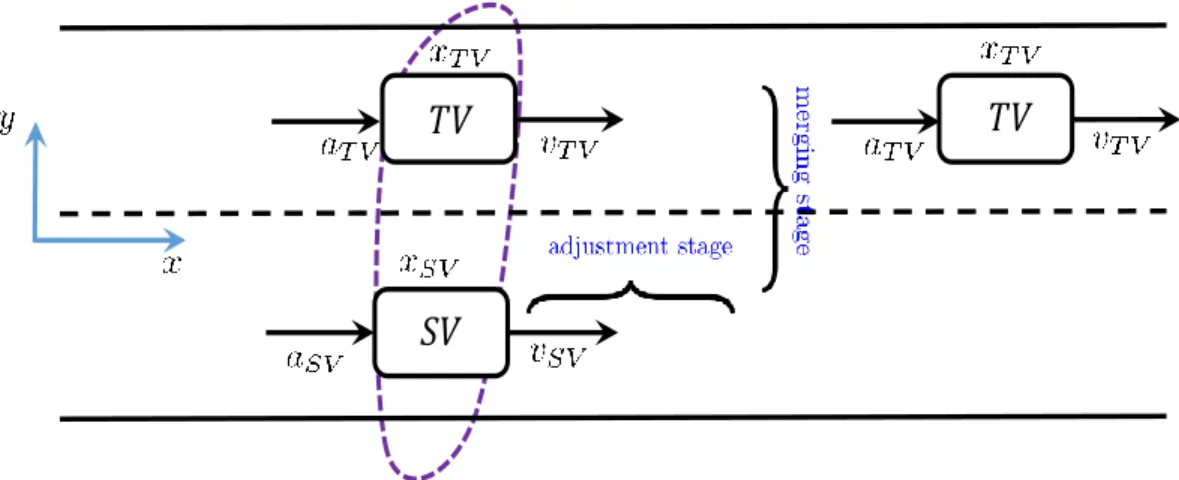
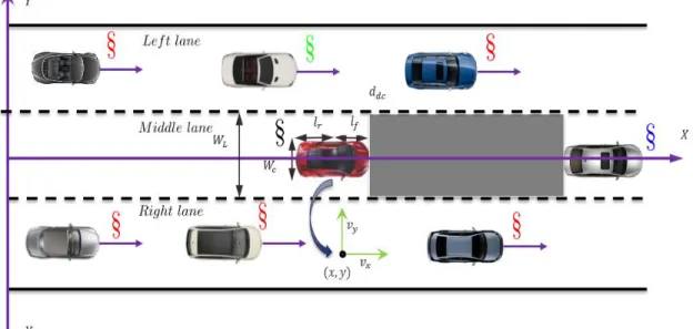
2.1 System model with related traffic quantites of eachT V s. Notice that the relative distance values are defined from eachT V sand velocities are also shown for eachT V. . . 41
2.2 Gaussian membership function for relative position. Notice that the cen-tering of each linguistic label is defined en terms ofSV speed. . . 43
2.3 Gaussian membership function for relative velocity. Notice that the
cen-tering of each linguistic label is defined en terms ofSV speed. . . 44
2.4 Gaussian membership function for cruising velocity. Notice that the cen-tering of each linguistic label is defined en terms ofSV speed. . . 44
2.5 Gaussian membership function for threat . . . 45
2.6 A cartesian coordinate is assigned for each vehicle. . . 50
2.7 This graph is intented to show the visual set-up with two camera orienta-tions. Green vehicles denote theT V sin the left lane, light blue vehicles are theT V sin the right lane. Animation is seen at 2 seconds . . . 50
2.8 Animation snapshot at 12 seconds . . . 51
2.9 Animation snapshot at 33 seconds . . . 51
2.10 Accelerations of vehicles . . . 52
2.11 Positions of vehicles . . . 53
2.12 Velocities of vehicles . . . 53
2.13 Threat of vehicles in left lane . . . 54
2.14 Threat of vehicles in right lane . . . 54
2.15 Markov chain with 16 states . . . 56
2.16 An MDP with 16 states . . . 57
2.17 Scenario description . . . 58
2.18 Lane changing model . . . 59
2.19 Solution of MDP . . . 62
2.20 A Markov game with multiple agents . . . 67
2.21 Example of equilibrium . . . 69
2.22 General non-zero-sum Markov game set-up with multiple agents . . . 70
2.23 Markov game matrix . . . 72
2.25 A cartesian coordinate system is assigned to all the vehicles. The quantities such as length and width of cars are same for all vehicles, which is only
depicted onSV. . . 88
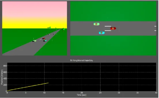
2.26 This graph is intended to show the visual set-up, with two different camera orientations of the simulated traffic. First, the SV starts with an initial speed of 22 m/s and it encounters an obstruction in its drive lane and searches for a gap. . . 90
2.27 SV turns on the turning signal and adjusts its speed in order to merge the gap ahead of T V2. Even thoughT V2’s objective is to prevent SV from lane changing,SV seeks to maximize the lower bound ofT V2’s action . 91 2.28 This is a cooperative case whereSV turns on the turning signal to the right gap in ofT V4andT V yields toSV for lane changing. . . 92
2.29 AsSV merges, T V4 decelerate to open a larger gap to merge in, conse-quently, eases the lane change process. . . 92
3.1 Schematic view of vehicle lateral dynamics . . . 96
3.2 Control structure of a lane change maneuvering . . . 99
3.3 Weighting control structure . . . 101
3.4 Input shaping filter . . . 104
3.5 Disturbance profile . . . 106
3.6 Control inputs . . . 107
3.7 Reference tracking . . . 107
3.8 Yaw angles . . . 108
3.9 Vehicle dynamical model . . . 110
3.10 Cornering force forµ=[0.1, 0.3, 0.5, 0.7, 0.9 . . . 113
3.11 Cornering stiffness forµ=[0.1, 0.3, 0.5, 0.7, 0.9 . . . 114
3.12 The control system structure . . . 116
3.13 Weighting control structure . . . 117
3.14 Tire cornering stiffness change in road profile . . . 122 xv
3.15 Wind disturbance . . . 123
3.16 Commanded steering . . . 123
3.17 Yaw rate outputs . . . 125
3.18 Slip side angle outputs . . . 126
3.19 Yaw moments . . . 126
3.20 Yaw rate vs steering . . . 127
3.21 Triangular membership functions . . . 129
3.22 State-feedback tracking controller . . . 133
3.23 Commanded steering for double lane changing . . . 137
3.24 Yaw rate outputs . . . 139
3.25 Slip angle outputs . . . 139
3.26 Yaw moment . . . 140
LIST OF TABLES
TABLE Page
2.1 Fuzzy inference rule table . . . 48
2.2 Design parameters used in simulation . . . 55
2.3 Design Parameters Used in Optimization . . . 87
2.4 Initial conditions of vehicles for scenario1 . . . 89
2.5 Initial conditions of vehicles of scenario 2 . . . 89
3.1 Vehicle parameters . . . 108
3.2 Vehicle parameters . . . 124
3.3 Fuzzy Rule Table . . . 131
3.4 Vehicle parameters . . . 138
1. INTRODUCTION AND LITERATURE REVIEW
1.1 Background
Even with the enhanced safety measures integrated in modern vehicles, the increasing number of vehicles on roads continues to produce a large number of traffic accidents on a yearly basis. In the last decades, autonomous driving has been a popular research area both in industry and academia. One of main objectives of autonomous vehicle research is to prevent the accidents caused by human errors. Because the traffic collisions are still one of the leading causes of deaths in entire world. In 2016, there were 40,200 people killed and 2 million more were injured in motor vehicle crashes in the United States [1]. The financial effects of the road crashes to the USA is a total cost of $432.5 billion per year, an increase of 12%from 2015 [1]. In this regard, the car manufacturers have offered a variety of safety systems in their cars that range from the adaptive cruise control to lane depar-ture warning system and anti-lock braking systems.Some other examples include braking assistance systems [2, 3], traction control systems [4], collision warning systems [5], lane-keeping systems, and lane change support [6, 7]. Research studies in active safety system design does not only involve automation of individual vehicle subsystems, but also in-cludes improved functionality of sensing and decision-making. The introduction of sensor technology in vehicles has enabled new possibilities of providing information concerning vehicle surroundings. This information is used to identify obstacles on the road that can be further analyzed by a decision-maker to execute the best possible actions such as a lane change or braking to avoid an accident. In the case of references on a roadway, the sensing systems are classified into two categories [8]: look-down and look ahead systems. Look-down sensing systems (either electrified wires or permanent magnets) have the advantages of being reliable, yielding accurate results and good performance under different weather
conditions. Richard Bishop addresses the above considerations in his paper [9]. The paper mentions about the main components in autonomous driving technology, including the ve-hicles vision systems, radar systems as well as the applications in adaptive cruise control and collision warning systems.
Intelligent transportation systems (ITS) is a premier forum that covers a variety of ap-plications. I primarily focus on human-vehicle interaction in automotive systems. There-fore understanding human behavior is the main pillar of above autonomous driving tech-nologies. The topic of human drivers has been studied in the literature [10]. It is important to point out that there is no comprehensive method that captures of all human behaviors. However, several contributions have been made to the field in the recent decades. Hancock et al. [11] explains the human factor in Intelligent Vehicle and Highway Systems design. The main focus on sense of safety in driving. Second issue addressed is drivers work-load such as navigation of traffic, vehicle controls and collision avoidance. Several tasks combined makes a reliable and safe design challenging task. Parkeret al.[12] investigate driver errors and violations. Tendency to a make error is divided in two parts; drivers mis-judgment and experience and deliberate driving violations. Salvucci [13] explores human driver cognitive architecture for control and decision making. The model discovers the limitations of general human abilities in driving domains. Trulls Vaa [14] explains percep-tion of risks, the consciousness in driving, as well as cognitive human driver models. [15] examines human drivers in dynamics and control point of views. Human belief state deter-mines the responses to a given traffic situation [16]. The decisions are simply made based on the perception of a driver, which mostly rely on subjective reasoning process [17]. A decision is made by a driver at each instant of time. As soon as a decision is made, an action of accelerating, decelerating or keeping the current state of the vehicle is performed by the driver. Human driving factor, therefore, has significant influence on driving. For example, the gender and age have important differences on driving style as well. One can
claim that the safety is directly related to the age of the driver since the young drivers pose more aggressive style than that of old drivers.
With this regard, It is quite essential to approximate a driver’s intention to a real time driving with a set of logical decision methods. This is to say, I develop a stochastic de-cision reasoning method based on a set of established logical driver perceptions for an emergency lane change problem. The model relies on a Fuzzy Markov Decision process based discrete dynamics and a Quadratic programming based MPC control for appropriate maneuvers to avoid accidents. The trajectory is then followed by a controller wherein a nonlinear vehicle model and a Linear Parameter Varying controller are employed. Overall system forms a hybrid system structure to approximate the human reasoning process to the actual mechanical output of the vehicle.
1.2 Objectives
In this work, we focus on designing an active safety system with a two level structure with a driver decision model algorithm that addresses the problem of avoiding obstacles in a lane in a three lane highway driving environment, and a driver driving model that performs a lane change task to a desired lane by combining several theories in the field of study. The driver decision model executes a decision based on stochastic reasoning of human with the fuzzy Markov game (FMG). This step determines an action with the most beneficial to the driver (highest safety), also the the target lane as well as the target velocity of the subject vehicle by taking into account the interactions with surrounding vehicles. The target outcomes are fed to a trajectory generator where the subject vehicle’s motion is planned. The combined assessment of the designing is performed in several driving simulations.
The next objective is to be able to follow this trajectory with the highest accuracy in a real driving scenario. With this regard, I consider a real vehicle dynamics model
𝑘 + 1
𝑘
Figure 1.1: Driver model of an autonomous vehicle
and controller design to follow the online generated path in a simulation model. The driver driving model has the actual dynamics of a vehicle and a mechanical controller to follow the reference trajectory with the highest accuracy. The overall design includes the techniques of the artificial intelligence, the convex optimization and the robust control concepts to create an emergency lane change active safety system in highway driving.
1.3 Background and Literature Review
1.3.1 Driver Decision Models (Higher Level Controller)
Understanding of a human driver behavior has been an attractive topic to many re-searchers. With the high demand of the mathematical models in accordance with different kinds of applications, there has been a variety of driver models proposed. Some of the demands to be mapped in driver models are listed as;
DRIVER STATE COLLISION PREDICTION MULTI-PHASE TRAJECTORY GENERATION HUMAN INTENTION VEHICLE CONTROL VEHICLE DYNAMICS Driver decision model Driver cognitive model Driver driving model
Figure 1.2: Schematic diagram of the proposed driver model
• General driver skills, information perception and processing, time delays, preview, adaptation,
• Learning and planning ability (path and speed adjustments), • Types of drivers such as experience, age, and aggressiveness,
• Features like emotions, concentrations and driver’s psychological state etc.
Depending on the application discussed above, several ideas have been proposed. One major aspects of the proposed models lies down on mathematical modeling such as using control theory (transfer functions, optimal and adaptive control), fuzzy logic, and neutral networks -hybrid approaches, which generally lead to differential equations. We will start the discussion of the problem of driver modeling from classical transfer function models to fuzzy logic and game theoretical based modeling as well as stochastic models such as Markov models.
Considering a design of an advanced driver assistance system, it the main aim of in-vestigation to form the overall design as automobile-driver coupled system. After defining driving task and environment where it is indeed necessary to introduce the traffic dynam-ics into the design. We can write down the main concerns of analysis with the following headlines
The vehicle:
design and control of vehicle components; including vehicle dynamics and material design of subcomponents.
The driver:
understanding individual driver as well as interaction of the drivers in a traffic situ-ation; path and velocity planners; subjective driver behaviors for decision making.
The environment:
traffic flow; influence of other traffic participants; modeling of the traffic system.
The combined system:
accident possibilities; accident prevention; driver support and learning tasks.
The extensive driver models built based upon individual driver behavior (i.e., miss-ing driver interaction dynamics) are available in the literature. Most of developed models have considered to control lateral vehicle dynamics while longitudinal dynamics is often thought to follow a given speed profile (i.e., car following models are shown in the up-coming subsections), independent of steering task of the driver. Plöchlet al.[18] explain several driver models in their paper. This dissertation introduces some of the models as background information in the field. Kondoet al.introduce one of the fundamental driver modelings in the literature [19]. They considered a 2-wheel vehicle model on a straight way with constant velocity and wind disturbances, Kondo’s model adjust the vehicle’s position by steering to a point with which the vehicle centre line coincides. A preview distanceLis defined in the reference. The main idea is to reduce the deviation∆yvehicle in
a distanceLahead of the vehicle i.e., looking-ahead distance. The relation of the figure is defined with the following equation
∆yvehicle ≈y(t) +Lψ(t) = y(t) +Tvehiclevψ(t)≈y(t+Tvehicle) (1.1)
where preview time Tvehicle = L/v, vehicle speed v, yaw angle ψ(t) and deviation is definedy(t). The changes on the lateral deviation i.e.,∆yvehicleis interpreted as the change
on the lateral direction with respect to the preview time i.e.,y(t+Tvehicle)From a control theory point of view, a proportional steering control strategy, C(s) = K leads to the steady-state error to zero i.e.,∆yvehicle = 0. In [20] another human tracking based model
𝜓𝜓 ∆𝜓𝜓 ∆𝑦𝑦𝑣𝑣𝑣𝑣ℎ𝑖𝑖𝑖𝑖𝑖𝑖𝑣𝑣 𝑅𝑅𝑅𝑅𝑅𝑅𝑅𝑅𝑅𝑅𝑅𝑅𝑅𝑅𝑅𝑅𝑅𝑅𝑡𝑡𝑅𝑅𝑡𝑡𝑡𝑡𝑅𝑅𝑅𝑅𝑡𝑡𝑡𝑡𝑅𝑅𝑦𝑦 𝑆𝑆𝑆𝑆𝑆𝑆ℎ𝑡𝑡𝑝𝑝𝑡𝑡𝑆𝑆𝑅𝑅𝑡𝑡 𝑦𝑦(𝑡𝑡) 𝑉𝑉𝑅𝑅ℎ𝑆𝑆𝑅𝑅𝑖𝑖𝑅𝑅𝑡𝑡𝑅𝑅𝑡𝑡𝑡𝑡𝑅𝑅𝑅𝑅𝑡𝑡𝑡𝑡𝑅𝑅𝑦𝑦
Figure 1.3: Kondo’s driver model
C(s) = K(TLs+ 1) (TIs+ 1)(TNs+ 1)
e−τrs (1.2)
In this model, human reaction time is givenτrand the neuromuscular delay time isTN are human properties, perform independently from the task. The other parameters K, TL, TI are associated with system. Kondo later introduced a second driver model that presents a linear deviation of the yaw angle and lateral position. This is an inspiring model, which have been modified and used in the literature. Another driver model is proposed in [21, 22]. The main idea is to compensate the deviation of the lateral position of the vehicle∆yvehicle,
with respect to a reference target position and the yaw angle error.
There are approaches in driver modeling that take into account when the road is straight and curvedρr. One of the works [23] Reid et al. define the steering control law as follows
δc =Kcρ?r+Kψ∆ψe+Ky∆ye (1.3)
�
Reference
Sight Point Human
Transfer Function Controlled Vehicle Dynamics + − Visual Error Steering Output Position Closed-loop Transfer Function
Open-loop Transfer Function
Figure 1.4: Transfer function of driver model
whereρ?
r is the road curvature point ahead, which will be previewed by the car after the preview timeTP, the difference between the vehicle heading angle and the heading angle of the roadway at a point is∆ψe, and∆yeis the distance from vehicle’s center line to the lane center-line at a point.
Based on the driver models, the human regulation control tasks are studied in frequency domain [24]. The open-loop transfer function i.e.,C(s)G(s), which the combined form of driverC(s)and vehicle dynamicsG(s), is described the crossover model with
C(s)G(s) = ωc s e
−τrs, (1.4)
that imposes a behavior amount of −20dB/decade in the magnitude due to the integral, and a phase shift −900 around the crossover frequency ωc. Even though human driver
is capable of compensating tracking errors regardless of vehicle characteristics, the input excitation signal restricts the crossover model behavior, especially in high gain at different driving maneuvers.
The idea of combined driver models, which has two-level structure is not a new idea proposed in the literature. Donge in [25] proposed a two level model where the road characteristics and a driver model form a layer, separated from the vehicle dynamics. He defines an anticipatory loop and a compensatory closed-loop control. The open-loop control determines the anticipatory steering response to be able to run of the path curvature. The parameters of interests in this layer are estimated by measuring the desired path curvature and the steering angle of the driver. Donge also suggest that human driver anticipate the change in road curvature and initiate front steering before the curve begins. A differential equation to model of the required anticipatory steering angle is proposed in [26]
T22δ¨a(t) +T1δ˙a(t) +δa(t) = Vaκ(t+Ta) (1.5) whereTais the anticipation time andκis the desired path curvature. In order to determine the open-loop steering angle to follow a given trajectory with high accuracy for a 2-wheel vehicle model, the parametersT2, T1andVaare set as the functions of vehicle parameters
and speed. In the compensatory closed-loop control level is responsible of stabilization of the driver steering wherein actual and desired path curvature is compared, i.e.,∆κ, along with the observation of the heading angle error of the vehicle∆ψ and lateral deviation of the vehicle∆y. The mathematical formula of the compensatory steering angle is
δc(t) = −[hk∆κ(t−τr) +hψ∆ψ(t−τr) +hy∆y(t−τr)]. (1.6) where τr is the lag of human driver, and the gains , hκ, hψ, hy are computed based on the measurement difference, open-loop control contribution, and minimizing a quadratic function.
Taking into account the vehicle’s nonlinear dynamics, several nonlinear control meth-10
ods have been proposed to present a driver model in [27]. With a multi-level structure, in which a guidance level sets the reference trajectory and velocity profile of the vehicle to a target point. In the stabilization level, a position controller to force the current state of the vehicle i.e., current target point to a desired target point with a suitable steering wheel angle and brake/acceleration. In this level, the vehicle position onx, y axis is controlled by nonlinear front lateral tyre forces and longitudinal tyre forces, which allows one to simultaneous control of lateral and longitudinal dynamics.
Another type of modeling of a human driver is fuzzy logic control (FLC). The fuzzy logic control relies on analyzing input values in terms of logics that is resemble of human thinking process, and a useful tool process of decision making when the system structure is very complicated. In terms of application, there are fewer works in the literature. One of the leading works have been proposed in [28]. The overall structure of the control loop is drawn below. Assuming a complete preview information regarding upcoming road curvature on the reference, the controller is formed in feedforward, feedback, and gain scheduling rules. The inputs to the feedback rules are defined as the combination of state errors of the system, i.e.,[y,y,˙ ψ˙ −ψ˙d]the vehicle’s lateral error with respect to the road center, the lateral velocity error, and the yaw rate errors respectively. The inference rules consist of linguistic variables LE (associated with y), CLE (associated with y),˙ Y W R (associated withψ˙ −ψ˙d), and∆F B (associated withδf b). A feedback rule is given with the following form:
IFLEisALE AN DCLE isACLE AN DY W RisAY W RT HEN ∆F B isA∆F B (1.7) where linguistic values ofAi,
ALE ∈ {N B, N S, N IL, P S, P B}, ACLE ∈ {N B, N S, N IL, P S, P B}, AY W R ∈ {N B, N S, N IL, P S, P B},
A∆F B ∈ {N H, N B, N M, N S, N IL, P S, P M, P B, P H},
with the 5 different subsets forALE, ACLE, AY W Rare given (N B ⇒negative big,N S ⇒ negative small, N IL ⇒ nil P S ⇒ positive small, P B ⇒ positive big) with triangular membership functions. Therefore, 53 = 125 rules in feedback rule base. For defuzzi-fication, 9 subsets with 4 new different subsets given ((N H ⇒ negative huge, N M ⇒ negative medium, P H ⇒positive huge,P M ⇒ positive medium) that results in a crisp steering angleδf b.
A wheel steering preview angle termδpris generated with respect to preview weightp divided by the future curvatureρ, over preview time window [28]. Consequently, theδpr takes the form
δpr = pc ρc
+pn ρn
(1.8) where pc and pn are the current and next radii of curvature preview parameters, respec-tively. The detailed information on selection of the parameters is given in [28].
The final steering wheel angle based on the feedback rule base and the preview rule base is determined in the gain scheduling rule base by taking into account the vehicle speedv. There velocitiesv1 = 5m/s, v2 = 12,5m/s, andv3 = 20m/s are introduced in
the feedback and preview rule bases and the gain scheduling rule is therefore defined
IF V isAV T HEN δc=δf bi +δpri , (1.9) 12
whereAV ∈{small, medium, big} atvi(i= 1,2,3). More details can be found [28]. Moreover, the artificial neutral networks (NN) is a powerful tool to present a human driving behavior. A longitudinal model, based on NN, is studied in [29] where the goal is to follow a reference velocity in different driving cycles. A block diagram is shown below. Two NN controllers are responsible for different goals. The fixed NN is to model a driver for reference velocity followingr(t). The NN is trained with input/output data. The inputs are the error e(t) = r(t)−v(t), where v(t)is the velocity of the vehicle, r(t), preview velocityr(t+k1)k1 = 1.1sec, and the time delayed error e(t−k2) k2 = 0.4sec. The
adaptive NN controller functions with the driver model, as the name refers it compensate thee(t)with respect to the changes in road conditions.
Most of the models introduced above only considers modeling a human driver model are useful when the implementation only requires individual car behavior without tak-ing into account other cars actions. Current trend in autonomous drivtak-ing involves not an action of the vehicle determined for individual benefit but an action executed after the other cars behaviors have been assessed. This also opens a door to implement a control system structure for autonomous vehicles includes a two level structure where a higher level controller (driver model) assesses the uncertain driving environment, creates reference trajectories for the lower lever controller to follow, and provides safe driving along with fuel economy and comfort, while a lower level controller performs the com-manded actions. The autonomous vehicle has several features that are associated with drivers behavior when they encounter varying traffic situations. A higher level controller or so called driver models offer an approximation of a driver behavior. This module is also called planning route. As the name denotes, route planning (i.e., the state in which the vehicle be in the next time step), and behavior decision-making (i.e., discrete values of the states wherein a continuous decision is produced at each time step) are main elements of this module. Route planning generates safe driving areas for autonomous vehicle. The
behavior decision-making provides reasonable driving actions such as turning left, turning right as well as accelerating and decelerating turning in different directions based on how the driving environment is defined. Yoo and Langari in [30] presented a game- theoretic risk estimation of the other cars behavior and corresponding time evolution of the col-lision areas. A predictive driving controller successfully avoids the colcol-lision area based on the subject car’s safety assurance level. They first define the relative dynamics of two interacting vehicles, attached relative to the vehicle of interest. A hybrid model is formed such that lane change decision leads to two modes, i.e., approaching the adjacent lane and stabilization in the adjacent lane.
fapproach = K T (x+a), fstabilization =− K T (x−b) (1.10)
where T denotes the period of lane changing, K, a, b are related to model parameters. Incorporating the driver’s aggressiveness, an aggressive driver is assumed to complete a lane change task in shorter time. A discrete forward reachable set analysis forms an unsafe region for the subject vehicle. A non-cooperative Nash game along with an utility function in driver’s decision model is employed to estimate the player’s driving strategy according to the subject vehicle’s strategy and the hybrid mode of the system. Model predictive control adjust the longitudinal control of the subject vehicle to stay outside of the collision region. The optimization is given
minimize u J = Z tf t0 (xTQx+uTRu)dt subject to x˙ =f(x, u), x1(t0), x1 ≥Cv,upper∨x1 ≤Cv,lower, x2(tf) = 0, amin ≤u˙ ≤amax.
whereJ is the quadratic cost function with weightsQ, R, the period for the cost function to be minimized [t0, tf], f(x, u) denotes the system dynamics with x is velocity and u is control input, Cv is the collision cross section area inR2. Simulations are performed for timid and aggressive drivers. The subjective collision perception for different types of drivers affects the recognition of risk and driver’s driving controller allows the subject vehicle to stay outside of the region.
Perception Belief Emotion Conscious
Input from
the senses Behavior
Figure 1.5: A schematic process of a human like decision making. Human brain collects the information from environment and processes based on a subjective reasoning process and executes an output according to the current state of cognition.
Neutral networks is another approach used in autonomous driving. The neutral net-works is often called as black box. It can function as controller after a sufficient training process. Shai Shalev-Shwartz et al.[31] proposes a neutral network based driving strat-egy where the system is trained with real time data. Then the future behavior of the cars can be easily predicted. Kim and Langari use a higher level decision strategy where the analytic hierarchy process (AHP) is used to by evaluating driving safety, traffic flow, and the fuel economy simultaneously in [32]. The proposed adaptive AHP is able to handle the decision making process under different traffic situations and driving modes.
The driving is an uncertain dynamical process. It is quite hard to create a determin-istic driver model due to uncertainty of the driver behavior under different environments. Markov Chains is a promising tool to predict driver behavior in such cases. A discrete Markov process is a stochastic process that satisfies the Markov properties. The discrete Markov process produces transitional probabilities of a finite number of future events with-out any knowledge of the past events. The fact that the next event only depends on the present event is one of the key properties of a Markov process. The term one-step tran-sition probability is used to define the conditional probability of visiting a particular state in the next transition given the current state [33]. We first define the state of the system at timetasS(t). A set of finite number of states is indexed by integers from 0 to n. Let us denote P(S(t) = i) be the probability of being in state iat ttime. And Pij denotes the transition probability of statej given that the current state is in stateiat timet.
P(t) = P00(t) P01(t) . . . P0n(t) P10(t) P11(t) . . . P1n(t) .. . ... . .. ... Pn0(t) Pn1(t) . . . Pnn(t)
In [34], the authors proposed a stochastic driver model based on Markov Chains. Ex-16
perimentally collected data is used to estimate the transition probabilities that lie in a con-vex uncertainty set. The model predicts a set of trajectories in the subsequent time interval for different environments and states of the vehicle.
1.3.2 Markov Decision Process (MDPs)
We can divide the decision making into two categories; the deterministic and the stochastic decision outcomes. For the stochastic outcomes, the different outcomes have different utilities. A good decision making weights the all these outcomes utilities to the probabilistic numbers. Human reasoning relies on a decision making with several out-comes. The quality of an outcome is subjective i.e., It depends on the human perception. With this regard, modeling of the human decision model with a set of outcomes is a good approach in a decision process. Since the quality of a decision is determined by a particular driving conditions i.e., a rational decision might result in a good outcome in normal driv-ing condition while a rational decision might lead to an accident in an abnormal drivdriv-ing condition, a decision made by human drivers associated with stochastic outcomes will be the ground of our research activity. For lane changing maneuver, the driver is influenced by surrounding vehicles behaviors. This means that the likelihood for specific outcomes is determined by the vehicles in neighboring lanes.
The main decision considerations for a lane change maneuver in an obstacle avoidance are the followings:
1. Which gap to choose for merging in neighboring lanes. 2. When to initiate the actual maneuver into the gap. 3. If the maneuver is able to performed.
𝑢1 𝑢2 𝑆1 𝑆2 (0.1,2) (0.9,4) (0.6,1) (0.4,5)
Figure 1.6: Illustration of an MDP with two states and two actions. The transition proba-bilities and rewards are given by tuples (p, R)
.
The outcomes of the decision is based on the probabilities and the utilities (rewards), so that the estimation of these set of numbers is crucial. In this work, It is assumed the sensor system has a perfect measurement. This means that the detection of the vehicles as well as the objects is unlimited. The sensor system also has the complete information of the velocities and relative positions of the vehicles to the subject vehicle. The objective of the proposed model and algorithm is to capture a human like reasoning of a decision to be made. In the solution process, some simplified assumptions are carried out. There is an assumed available gap as well as the detection of an object is drive lane is fully known. 1.3.2.1 MDPs in autonomous driving
Markov decision process has been used as a decision-making model in autonomous vehicle research. It has several features such as modeling the uncertainty with a set of probabilistic numbers, executing several possible actions in a given traffic condition, and being able to capture human reasoning that makes a logical selection among all possi-ble alternatives in a decision making process. In order to enhance the understanding the
MDPs, the basic concepts are demonstrated in this section.
Markov Decision processes (MDPs) are powerful tools for sequential decision in stochas-tic environments where an agent has to execute an action to achieve an objective. Execut-ing an actionu∈U, given the system is in a states∈S is defined as a policyϕ:s→u. In order to find such an optimal policy i.e., ϕ?, a linear programming or a dynamic pro-gramming equation is iteratively solved.
Brechtelet al.[35] consider a discretized MDP model derived from a continuous state-space model is proposed. They extend the discussion by including the uncertainties in the driving with the Partially Observable Markov Decision Processes (POMDP) in [36]. Their solution of the problem based on the position and velocity states of cars. Ulbrich et al. [37] consider the Partially Observable Markov Decision Processes (POMDP) to model the uncertain and dynamic driving environment for a single lane driving. They use a small set of 8 to describe the highway driving situations.The high computational burden observed in [35, 36] is solved with signal processing networks to simplify their POMDP solution. Even though their POMDP set-up can be practical, computation time remains a challenge and It is not suitable for online application in an emergency lane change decision making. Moreover, their work only considers a lane change into one gap and the selection between the gaps is not addressed. Weiet al.[38] presents a point-based Markov Decision Process algorithm is proposed as an approximate solution to the POMDP for a single lane au-tonomous driving behavior. The uncertain behaviors of traffic participants are considered to implement in a specific traffic situation. They introduce a set of cost functions to model the driving environment for decision making. Only a longitudinal control of the subject vehicle is considered in their work. These and similar higher level controller designs are increasingly being considered to both avoid and minimize accidents and as a prelude to fully autonomous driving systems of the future.
1.3.3 Game Theory
Game theory has been used widely as a decision maker in social sciences and in en-gineering field because of its advantage to model the interactions between players. There are mainly two types of games; cooperative and non-cooperative games. The first case where the players benefit from individual coalitions, the joint action sum of collective ob-jectives of the players. In this case, the players receive information about their actions, subsequently exchange information of their payoff’s. The second case the objectives are conflicted where the players seek to achieve their own strategies regardless of what the other player gains. Moreover, a non-cooperative game is also characterized as the players do not exchange information about their individual actions, rather the decision are made independently.
1.3.3.1 Game Theory in autonomous driving
Game theory is a promising decision making for autonomous vehicles where It does not only predict the subject car’s behavior but also evaluates and sets up a game according to the surrounding vehicle’s behavior i.e., the lateral and longitudinal movement, or more complicated movement can be considered simultaneously. A cooperative multi-agent sys-tem is modeled by combining the individual cost function into a team cost function in [39]. Nash-bargaining solution is proposed for minimum individual cost by maximizing the difference between cooperative and non-cooperative cases. Kita in [40] developed a game theoretic interactions model of cars in a merging-giveaway scenario. A pair of merg-ing and through cars interaction is explicitly considered, which they take the best actions from their perspectives, thus the game forms a two-person non-zero-sum non-cooperative game. In [41], the authors considered a lane-changing model in a connected environment where the notion of incomplete information is utilized in a two-person zero-sum non-cooperative game solution. Wang et. al in [42] proposed a differential game where the
controlled vehicles execute decisions according to the expected behaviors of other vehi-cles. In this work, two game solutions are proposed; non-cooperative game where the vehicles optimize their own costs and cooperative game where the collective cost function is optimized with coalitions. Yuet al.in [43] consider a human-like game theoretic model of lane changing involving interaction with surrounding drivers using the turn signal and lateral moves and their aggressiveness. In [44], dynamic lane change decision making is performed by utilizing the idea of Receding Horizon control. The decisions are updated as new information is available to the autonomous vehicle. Some other examples of the design of the higher level controller using the Game theory for autonomous lane changing in [45, 46] where a subject vehicle and the other traffic participants determine their actions within an optimization framework. In [46], the authors set up a scenario where the cars are driven on a 3-lane highway environment. They establish an action space as follows;
1. Maintain current speed
2. Accelerate to a speed up to110km/h 3. Decelerate to a speed up to50km/h 4. Move to the left lane
5. Move to the right lane
It is important to note that the actions provided by a higher-level controller in which the action commands are fed to a lower level controller to be performed by vehicle level dy-namics and controller. A reward function is defined as summation of driver interests.
wherewi,i= 1,2,3are the defined weights for the termsccollision,hheadway,eeffort. For more details how these terms are defined, please see [46] . In this work, the driver’s policies are stochastic and two approaches are employed for mapping. Level-k approach and Jaakkola reinforcement algorithm. Main idea behind this, to obtain a driver policy that relies on the observation and interaction of the other drivers in traffic. Simulation results assess the effects of driver aggressiveness on the number of collisions and lane changes.
1.3.4 Trajectory Planning for Autonomous Vehicles
The problem of trajectory/path planing has been extensively researched in the litera-ture. Path and speed planner can be seen as an internal driver task, which can be incor-porated in the driver model. Many driver models require a desired path to follow, which is either assumed to be given or generated by a separate tool. Apathis defined as a con-tinuous sequence of configurations that connects an initial configuration to a terminating configuration [47]. In other words, a path is a geometric line on which the vehicle follows in order to reach a final point without colliding an obstacle. A path-planningalgorithm then computes a feasible trace of a geometric configuration for an autonomous vehicle such that the design constraints i.e., road limits, vehicle dynamical limits, and traffic rules etc..are satisfied. Amaneuvercharacterizes the motion of the vehicle in a road geometry. Some examples of maneuvers include ’turning right’, ’turning left’, or going straight’. On the other hand, thetrajectory planningconcerns a vehicle’s motion in real-time from one possible state (velocities and positions) to another by satisfying the vehicle’s dynamics constraints, safety constraints, design constraints as well as the rules of traffic [48]. In this regard, trajectory planning (or trajectory generation) is divided into sub-levels;
1. Finding the best path according to the vehicle dynamics limits to follow. 2. Finding the best maneuver to perform under constraints.
𝒀𝒀
𝑿𝑿 𝒙𝒙𝟎𝟎,𝒚𝒚𝟎𝟎
𝒙𝒙𝟏𝟏,𝒚𝒚𝟏𝟏
𝑶𝑶
Figure 1.7: An example of a path .
3. To be able to avoid an object in traffic.
4. Adapting the planning of a path according to the sudden change in traffic.
Vehicle kinematics and road entities have been considered in all existing studies. This is a founding element of path planning - trajectory generation problem in autonomous driving. A high amount of research has been made in trajectory generation for longitu-dinal and lateral movement for vehicle following as well as avoiding obstacles. Most of the works in the fields consider a lane change decision has been made by a higher lever controller or a driver decision model, then a feasible trajectory is computed satisfying the design objectives [49, 50]. Nilsson et al.[51, 52] consider utilizing a point-mass vehicle model to compute a maneuver in vehicle’s longitudinal and lateral direction as well as a longitudinal velocity profile by using Model Predictive Control (MPC). Then the planned path is followed by a lower level controller wherein the vehicle dynamical model and a
Nonlinear Model Predictive Controller are employed. The trajectory generation is formu-lated within quadratic programming where the longitudinal and lateral control objectives are satisfied simultaneously. They introduce the Forward Collision Constraint (FCC) and the Rear Collision Constraint (RCC) as linear inequality constraints to avoid a crash with a car in the drive lane. Rosolia at al. [53] consider a point mass model and an MPC in outer loop to generate a collision free track and Proportional Integral (PI) control and bi-cycle model are used to track the trajectory in inner loop. Hosseini et al. [54] proposes an adaptive collision warning algorithm that supports the driver for collision avoidance. Their solution relies on two main functions; the first function is to generate a feasible trajectory based on the vehicle and road limits, a steering is performed for a safe lane change, the second function is to trigger an alarm signal to the driver when required. In their optimization solution, a bicycle model of a vehicle is employed. The steering control input is minimized by simultaneously satisfying the systems dynamics as well as design constraints.
1.3.5 Longitudinal Vehicle Control
An autonomous vehicle is required to perform two main tasks, i.e. to maintain a safe longitudinal spacing relative relative to the leading vehicle and to control the lateral mo-tions of the subject vehicle [55]. The technical discussion to identify the longitudinal control behavior of drivers are sparse as compared to the works about lateral control be-haviors in the literature. Longitudinal spacing of vehicles are particularly important from the safety point of view. The spacing is measured by the physical dimensions of the vehi-cles as well as the gaps between them. To this end, two microscopic measures the distance headway and distance gaps are widely used. These quantities are used to characterize an important concept in transportation community, so called car following models. Car following models produce an acceleration of the vehicle, which subsequently establishes
an effective traffic simulations, based on relative position, relative velocity, the velocity of the autonomous vehicle as well as lag in perception. One of the commonly used car following models is the General Motor’s model, which is proposed by Gaziset al.[56]. In this model, the motion of the subject car is governed by an equation, the acceleration is the response of the model. Another model is the Gipp’s car following model, proposed by Peter G. Gipps [57]. This model ensures a safe distance between the subject car and the car in front of it. The GM’s model fails to consider in this regard. Optimal velocity model [58, 59] is defined that each driver tries to obtain an optimal velocity based on the relative distance and velocity. This is a dynamic model that the car’s acceleration is pro-portional to it’s optimal speed and actual speed. The intelligent driver model (IDM) is also a well-known car following model, proposed by Treiber et al. in [60, 61], produces an acceleration as a continuous function of the velocityvα, the velocity difference∆vα, the net distance gaps?.
Figure 1.8: A car following model in highway driving. The subject car is in the middle, and the front vehicle is the lead car. The subject vehicle reacts to the change in the speed of the lead car. The rear car also reacts to the speed change of the subject car.
˙ vα =a " 1− vα v0 δ − s?(vα,∆vα sα 2# (1.12) whereδand the maximum accelerationaare the model parameters.
There are several studies proposed to apply the above methods in advanced driver as-sistance systems. For example, Adaptive cruise control (ACC) is an extensively studied problem in the literature [62, 63, 64, 65]. Similarly to the car following models, a desired space and a velocity profile are obtained by continuously adjusting the vehicle’s accelera-tion profile.
1.3.6 Lateral Vehicle Control
Vehicle’s lateral behavior can be characterized in terms of lane change an merge op-erations [66, 67, 68]. For this purpose, researchers sometimes consider the lane change process as a decision making. Because a lane change depends on multiple objectives, such as speed profile, relative distance objectives before and after lane change as well as avoid-ing an obstacle in drive lane and a good reference trajectory to follow with high accuracy. Thus a lane change model should take into account several decision parameters. For ex-ample, Gipp’s has proposed a set of factors that leads the driver to change a lane. Ahmed et al. [69] has proposed a gap acceptance model to assess whether the drivers have min-imum acceptable gaps between the host vehicle and following vehicles. These methods have been well used in transportation research community.
For lane change control, the lateral dynamics of the vehicle is be considered. A refer-ence trajectory following is maintained by steering control [70]. Good set-point tracking of the trajectory during lane change does not only achieve safety but also improves driving comfort and fuel efficiency. In [71] authors model the nonlinear vehicle dynamics by an approximate hybrid affine model. They employ a time-optimal robust control algorithm to control the yaw rate and lateral velocity. In [72] authors implement frequency shaped lin-ear quadratic (LQ) control. Kim and Langari proposed [73] a neuromorphic strategy, and robustness of the design is investigated by altering the uncertain cornering stiffness. Hati-poglu et al.[74] a virtual yaw reference controller is considered and a robust switching
controller is utilized to generate steering commands for the vehicle to track the given ref-erence trajectory. Abe in [75] a human-driver model (HDM) based controller is proposed. A look ahead distance consistent with vehicle speed is considered.
1.3.7 H∞Based Linear Parameter Varying (LPV) Control
TheH∞control design finds a controller that provides both closed-loop stability and a satisfied level of performance index for reference tracking and disturbance rejection. Since
H∞is a disturbance rejection technique, the main purpose is minimizing the effect of input disturbance on the output of the system. TheH∞norm of a stable transfer function G(s) is the largest input/output root mean square (RMS) gain i.e.,
kGk∞= sup u∈L2,u6=0 kzkL2 kukL2 = sup ω σmax(G(jw)). (1.13)
The 2-norm, denoted bykyk2, is defined as
kyk2 ∆ = s Z ∞ 0 yT(t)y(t)dt.
Linear Parameter Varying (LPV) systems are described as the systems whose matrices are assumed to be affine with the variations.
G: ˙ x(t) =A(ρ(t))x(t) +B(ρ(t))w(t) z(t) = C1(ρ(t))x(t) +D(ρ(t))w(t)) (1.14)
Basically, LPV systems are expressed in terms of Linear Matrix Inequalities (LMI) , then the system matrices that are depend on the scheduling parameters are solved with currently available optimization methods [76]. The benefit of that technique is the infor-mation for all variations and the rates of variation in system are expressed in affine forms global optimization methods are used to solve them. These type of the systems are
con-trolled with the LPV controllers. LPV control is capable of measuring the the variations and schedule the system parameters accordingly. Lyapunov functions are the essential el-ement in order to establish stability and performance of the LPV gain scheduled systems. There are fixed Lyapunov functions, [77] or parameter-dependent [78, 79]. The latter con-dition simply means a parameter-dependent LPV controller used to control parametrically depended plant, whose parameter variation and rates are known. The second controller capture the whole variation during the process, therefore it provides less conservative ap-proach. A single Lyapunov functions may be used for a parameter varying plant. However, stability and performance specification may not be met in the closed loop system due to the arbitrary fast variation in the scheduling parameters. As a result, the system may not be internally stable for all variations. When the internal stability of LPV system is guaran-teed, the Bounded Real Lemma(BRL) condition is satisfied. A continuous differentiable matrix is sought such that the derivative of the matrix is decaying the zero exponentially. This simply gives the notion of the stability of the system.
1.3.8 LPV Control in Automative Research
There are three main control developments to achieve performance requirements in passenger cars. First is the ride comfort that is associated with acceleration sensed by passengers, second is the road handling that is related to alternations in tyre forces due to road surface changes, and the last one is suspension deflection that is associated with the body displacement of the car with respect to the road. The control of the these subsystems is always conflicting. I first review some of the relation works in suspension control do-main. The suspension control part can be categorized into passive suspensions, semi-active suspensions, and active suspensions controls. While active suspensions offer good ride, handling, vehicle posture, and stability than that of the counter parts semi-active suspen-sions, the energy consumption, cost, and complexity requirements are important negative
factors in implementation. Semi-active dampers fall into between passive and active sus-pension. The cost and installation are more beneficial as well as the feature of continuously controlled damping. The suspension system includes a damper or a shock observer that does not require much energy to operate. Within the limited context, I present some of the related literature works in control design perspective i.e., increasing ride comfort and road holding in view of road disturbances.
C. Poussot-Vassalet al.[80] proposed a semi-active suspension control. They first in-troduce a nonlinear quarter car model and experimentally obtained semi-active suspension system. Then the authors develop the internal stability and performance criteria within the LPV theory. The main contributions follow to fulfill the dissipative actuator constraint such that a type of robust norms (i.e., H∞ andH2) is established. The design is robust against model uncertainties. The design is computationally effective since it involves a simple scheduling strategy based on a static actuator model. Simulations and experimen-tal results are perform to fulfill theoretical findings. Anh-Lam Doet al.[81] give a quarter vehicle model with a semi-active damper in the LPV framework with nonlinear static semi-active damper model. The nonlinear static semi-active damper model presents the bi-viscous and hysteric behavior of the design. The dissipativity constraint is turned into input saturation that is scheduled in polytopic way. The input saturation problem is inte-grated with the initial model to synthesize the LPV controllers. Convex optimization based theH∞control design method is applied. The frequency and time domain results showed that the performance objectives as well as dissipativity constraint of the damper are simul-taneous achieved. M.Q.Nguyen et al. [82] consider the design of a semi-active suspension control problem based on Finsler’s lemma in the LPV state feedback framework. The de-sign first employs an LPV form of the suspension system and dissipativity constraints as generalized sector condition. Two different Lyapunov functions are used; one of the sta-bility and the other one for the disturbance rejection. Obtained polytopic system allows to
𝑚𝑚𝑠𝑠
𝑚𝑚𝑢𝑢
𝑧𝑧𝑠𝑠
𝑧𝑧𝑢𝑢
𝑧𝑧𝑟𝑟
(a) Passive suspension
𝑚𝑚𝑠𝑠 𝑚𝑚𝑢𝑢 𝑧𝑧𝑠𝑠 𝑧𝑧𝑢𝑢 𝑧𝑧𝑟𝑟 𝐶𝐶𝑡𝑡𝑅𝑅𝑡𝑡𝑅𝑅𝑡𝑡𝑖𝑖𝑖𝑖𝑡𝑡𝐶𝐶𝑖𝑖𝑅𝑅𝑑𝑑𝑡𝑡𝑚𝑚𝑝𝑝𝑅𝑅𝑅𝑅 (b) Semi-active suspension 𝑚𝑚𝑠𝑠 𝑚𝑚𝑢𝑢 𝑧𝑧𝑠𝑠 𝑧𝑧𝑢𝑢 𝑧𝑧𝑟𝑟 𝐹𝐹𝑡𝑡𝑅𝑅𝑅𝑅𝑅𝑅𝑡𝑡𝑅𝑅𝑡𝑡𝑎𝑎𝑡𝑡𝑡𝑡𝑡𝑡𝑅𝑅 (c) Active suspension.
Figure 1.9: Type of suspension systems
compute LPV controllers by using LMIs. Input saturation conditions and a performance comfort level are demonstrated as satisfying design objectives. The work [83] considers to mitigate the conflict between ride comfort and road-holding by allowing the continu-ous control of the damper force in the semi-active suspension systems. As the actuator saturation limits are enforced in the performance limits, their work is unique in terms of incorporating the actuator limits in form of saturation indicator parameters that is included in the LPV plant model. The LPV controller is synthesized using a full-vehicle model. As expected, the model leads to complexity of the controller compared to quarter vehicle suspension model. To solve this, the authors employ a disturbance-feedforward output-feedback controller to exploit the separation principle. This performance of the controller is compared with various types of existing methods in simulation study. Michael Fleps-Dezasse et al. [84] introduce a new scheduling parameter, called saturation transformer into the LPV plant. The saturation indicator and the saturation transformer capture the force constraint of the semi-active damper. The LPV controller is synthesized by gridding of the parameter space using a parameter dependent Lyapunov function. Different road profile excitations are used to show the benefits of the controller experimentally.
The LPV control design opens a door to tackle with parameter uncertainty and/or non-linearity of the system by converting it into parameter space. Inspired by this, A. Zin et al. [85] proposed an LPV/H∞ controller design with respect to suspension spring coefficient for active suspension systems. Their proposed control strategy compromises safety/comfort performances adapted online according to the driving situation. The con-trol design is in the view of global chassis concon-trol (GCC) framework wherein a switching control signal for ride comfort/road holding is produced with respect to the suspension subsystem. In [86] the design of an active suspension system in the LPV framework is also presented. The relative displacement between the chassis and wheel assembly is used to stiffen as the suspension limits are reached. TheH∞controllers ensure either passenger
comfort or suspension travel as the primary objective of the design. TheH∞ controllers are blended into the LPV controller, subsequently forms a nonlinear controller for the design of nonlinear active suspension.
Since the emergency lane changes involve severe driving maneuvers at high speed, the consideration of vehicle lateral stability generated by yaw moment is a must to create an overaly stable control system structure for an emergency lane changing intelligent system. The steering control methods are quite effective when the lateral tire forces are constant. The methods collapse when the vehicle tire forces reach saturation limit; resulting the loss of steer-ability leads to a high level accident possibility. Uncertainties in cornering stiff-ness as a result of tire-road friction efficient and vehicle load distribution affect the stability of the entire system. To solve this, researchers have proposed vehicle stability control sys-tems that mainly use direct yaw moment to keep the vehicle stable. Consequently, active front steering (AFS) system is combined with the direct yaw moment controller (DYC). In [87], coordinated control of AFS and DYC for stability and better vehicle handling is proposed. They employ an 8-DOF nonlinear vehicle model and tyre model. The authors develop a procedure based on an optimal guaranteed cost (LQR), and the effect of uncer-tainty on the cornering stiffnesses is discussed. The control objective to reduce the negative influence of the norm-bounded time-varying cornering stiffness uncertainty on the vehicle dynamics control with respect to the change in driving conditions. Hui Zhang et al.[88] considered the vehicle lateral dynamics stabilization problem with time-varying longitu-dinal velocity. The longitulongitu-dinal velocity is presented by a polytope with finite vertices and cornering stiffness is represented with norm-bounded uncertainty. An LPV model of the vehicle is introduced based on the varying longitudinal velocity and cornering stiffness. The control objective is to minimize the sideslip angle with a prescribed level of yaw rates. In the control design, a set of objectives i.e., the sideslip angle, yaw rate, and the control efforts, they propose a multi-objective energy-to-peak control withDstability. The same