Lifted Decimation, Labeling, and Counting
Dissertation
zur Erlangung des Grades eines
D o k t o r s d e r N a t u r w i s s e n s c h a f t e n
der Technischen Universit¨
at Dortmund
an der Fakult¨
at f¨
ur Informatik
von
Fabian Hadiji
Dortmund
2015
Dekan: Prof. Dr.-Ing. Gernot A. Fink Gutachter:
Prof. Dr. Kristian Kersting Prof. Sriraam Natarajan, PhD
I am thankful for the experiences that I was able to make and I am very grateful for meeting so many interesting and smart people during the time working on my PhD. I am very happy that the scientific exchange, as well as collaborations, with various people hold beyond the course of working on this thesis. Among all the people that I have met, I want to thank a few in particular.
First, I want to thank my supervisor Kristian Kersting for giving me the opportunity to start my PhD in the STREAM group at Fraunhofer IAIS. Besides being an inspiring supervisor with great advices, Kristian also brought a team of excellent researchers and great personalities together. It has been a great experience to work with the other members of the STREAM group and office mates. Kristan has always been very supportive and it was a pleasure to work with him on various papers and projects. On top of that, he is a person that is fun to work with.
None of the content in this thesis would have been possible without all the co-authors involved in working on the papers and writing the papers themselves. I have worked closely together with Babak in particular on various papers. The discussion with him were very resourceful and his vital contributions improved my own work greatly. Besides his contributions to research papers, I also want to thank Sriraam for his support and feedback during the writing of this thesis. A big thank you also belongs to Alejandro, Anders, Christian B., Christian T., Martin, Rafet, and Youness. These people contributed in unique ways to all of the published papers by bringing in their thoughts, ideas, and point of views.
The same holds for other colleagues with whom I have — unfortunately — not co-authored any papers: Mirwaes, Xiao, and Marion. Nevertheless, I have learned a lot from them. This also includes playing table football and I would certainly not underestimate the influence on research of winning matches in FIFA.
I also want to explicitly thank Christian T. and Anders. By hiring me at GameAnalytics, Christian widened my research interested to include analyzing user behavior in games and beyond. I met Anders through GameAnalytics which also resulted in fruitful collaborations up to this day. Both are still very helpful and I continue to enjoy collaborating with them in various areas.
I also want thank all institutes involved while working on my thesis which include the Fraunhofer IAIS, the University of Bonn, and the TU Dortmund University. Here, I also want to mention the University of Massachusetts Amherst. The research visit to Andrew McCallum’s research group has been another outstanding experience. Working together with such NLP experts, and in particular together with Sebastian Riedel, has been a pleasure.
There is another former colleague with whom I have not written any papers but received more support and help from than anybody else. Besides that, we share memories that go beyond research and work. Thank you for everything, Anja.
Besides all people I have met in past years at work, there is also a number of important people outside of academia that have supported me all my life. I want to thank my parents, family, and friends for their support and making life as great as it has been. I would certainly not write these lines without their continuous help and love.
The influence of Artificial Intelligence (AI) and Machine Learning on our everyday lives has been growing constantly over the past decades. Applications in both areas have attracted much attention and several of them depend on Probabilistic Graphical Models (PGMs). Furthermore, the emerging interest in methods originating from the Statistical Relational Learning (SRL) community has added to this underlying trend over the past ten years. In many cases, the combination of logic and probability is superior to relying on only either of the two. However, with problems becoming larger and more complex, inference and learning are still major issues in PGMs and in particular in the context of models derived from SRL formalisms. On the other hand, many problems in SRL are specified in such a way that symmetries arise from the underlying model structure. Exploiting these symmetries during inference, which is referred to as “lifted inference”, has lead to significant efficiency gains.
The idea of lifted inference is not solely applicable to relational probabilistic models though. We provide several enhanced versions of known algorithms that show to be liftable too and thereby apply lifting in “non-standard” settings. For example, we show how to use lifted message passing in a decimation procedure for solving satisfying problems. By doing so, we extend the understanding of the applicability of lifted inference and lifting in general.
The majority of research on lifted inference has so far been concentrating on PGMs with binary random variables. Certainly, these models are not the universal remedy to all problems in AI and in fact represent only a small subset of all PGMs. In many cases, we wish to model variables over a large domain, or even infinite range, even if this introduces new challenges to the complexity. Often, common formalisms become unsuitable and even efficient approximative inference is intractable. However, we can still transfer ideas from SRL and lifting to other approaches that are more suitable in this context. In this regard, we show that algorithms solving multiclass labeling problems can benefit from SRL-like weighted rules and lifted inference — which are both non-standard techniques in this area. Here, weighted rules induce sparse and symmetric problems from which Label Propagation, an effective labeling algorithm, can benefit.
We use our novel Label Propagation approach in combination with an innovative Web-based data harvesting pipeline to label author-paper-pairs with geographic information in online bibliographies. This results is a large-scale transnational bibliography containing affiliation information over time for roughly one million authors. By counting the number of migration hops of researchers, we can infer mobility patterns in migration from this database. We find distributions fitting the data well which have also been found describing human and social phenomena in other areas. In this line of research, we also show that the Web provides a rich set of additional data sources where similar patterns can be found in the spread of information and content on the Web. These findings share one commonality: all datasets were build upon counting.
Although counting is done literally everywhere, mainstream PGMs have widely been ne-glecting count data. In the case where the ranges of the random variables are defined over the natural numbers, crude approximations to the true distribution are often made by discretization or a Gaussian assumption. To handle count data with positive and negative dependencies, we introduce Poisson Dependency Networks (PDNs). PDNs are defined over a set of local probability distributions and we obtain a joint distribution via sampling, allowing us to answer various probabilistic queries. Additionally, PDNs do not only allow to describe dependencies between count random variables but also allow to make predictions for unseen instances. Hence, we provide a new class of non-standard PGMs naturally handling count data.
Acknowledgments i
Abstract iii
List of Figures ix
List of Tables xi
List of Algorithms xiii
1 Introduction 1
1.1 Illustrating “non-standard” PGMs and Lifted Inference . . . 3
1.2 Outline and Summary of Contributions . . . 8
2 From Probabilistic Inference to Lifted Message Passing 13 2.1 Probabilistic Graphical Models . . . 13
2.1.1 Factor Graphs . . . 17
2.2 Inference and Learning . . . 17
2.2.1 Exact Inference . . . 20
2.2.2 Approximate Inference . . . 21
2.3 Probabilistic Relational Models . . . 24
2.3.1 Markov Logic Networks . . . 27
2.4 Lifted Inference . . . 30
2.4.1 Belief Propagation and Its Lifted Versions . . . 33
2.4.2 Advanced Lifting Techniques . . . 41
2.5 Quality and Error Measures . . . 43
3 Lifted Message Passing Beyond Lifted Belief Propagation 45 3.1 Lifted Satisfiability . . . 46
3.1.1 CNFs and Factor Graphs . . . 47
3.1.2 Belief Propagation for Satisfiability . . . 49
3.1.3 Decimation Based SAT Solving . . . 50
3.1.5 Lifted Survey Propagation . . . 54
3.1.6 Lifted Decimation . . . 56
3.1.7 Experiments . . . 57
3.1.8 Summary . . . 59
3.2 Sequential Clamping . . . 60
3.2.1 Lifted Sequential Inference . . . 62
3.2.2 Experiments . . . 66
3.2.3 Summary . . . 69
3.3 Bootstrapped Inference with Lifting . . . 70
3.3.1 Lifted LM . . . 72 3.3.2 Bootstrapped LM . . . 74 3.3.3 Bootstrapped Lifted LM . . . 75 3.3.4 Experiments . . . 80 3.3.5 Summary . . . 85 3.4 Interim Conclusion . . . 86
4 From Lifted Message Passing to Algebraic Lifting 89 4.1 Label Propagation . . . 92
4.2 Lifting and Equitable Partitions . . . 94
5 Lifted Label Propagation 97 5.1 Logical Rules for Label Propagation . . . 98
5.2 Geo-Tagging Bibliographies . . . 98
5.2.1 Harvesting Data . . . 99
5.2.2 Inferring Missing Data . . . 100
5.2.3 Experiments . . . 102
5.3 Lifted Label Propagation . . . 103
5.3.1 Experiments . . . 105
5.4 Bootstrapped Label Propagation . . . 108
5.5 Learning Weights of Logical Rules . . . 108
5.6 Interim Conclusion . . . 110
6 Inferring Social Phenomena From the Web Based on Counts 113 6.1 Migration Analysis . . . 113
6.1.1 Related Work . . . 116
6.1.2 Sketching Migration . . . 117
6.1.3 Regularities of Timing Events . . . 118
6.1.4 Link Analysis of Migration . . . 124
6.1.5 Summary . . . 126
6.2 Other Social and Behavioral Phenomena . . . 128
6.2.1 Internet Memes . . . 128
6.2.2 Viral Videos . . . 129
6.3 Interim Conclusion . . . 130
7 Count Graphical Models 133 7.1 Related Work . . . 135
7.3 Learning Poisson Dependency Networks . . . 141
7.3.1 Poisson Log-Linear Models . . . 142
7.3.2 Non-Parametric Poisson Models via Gradient Boosting . . . 143
7.3.3 Multiplicative Gradient Boosting . . . 145
7.3.4 PRTs, Model Compression, and Dependency Recovery . . . 147
7.4 Making Predictions using Poisson Dependency Networks . . . 149
7.5 Experimental Evaluation . . . 150
7.5.1 Network Discovery from Simulated Data . . . 152
7.5.2 Cell Counts and Bibliography Data . . . 154
7.5.3 Bag-of-Word PDNs . . . 156
7.5.4 Communities & Crime and Click-Stream Data . . . 157
7.6 Relational Count Models . . . 161
7.7 Interim Conclusion . . . 163 8 Conclusion 165 8.1 Summary . . . 165 8.2 Lessons Learned . . . 167 8.3 Outlook . . . 168 Appendix 171 1 Selected Publications . . . 171 References 175 Index 193 Nomenclature 195 List of Abbreviations 197
1.1 Normalized Latin Square . . . 4
1.2 Lifted SAT Problem . . . 5
1.3 Lifted Labeling Problem . . . 6
1.4 PGM for Count Data . . . 7
2.1 Graphical Illustration of Different PGMs . . . 14
2.2 Example Factor Graph . . . 17
2.3 Grounded Smokers-and-Friends MLN . . . 27
2.4 Color Passing Illustration . . . 36
2.5 A Lifted Factor Graph . . . 38
2.6 Lifting of Factors with Variables at Different Positions . . . 40
2.7 Distinction of Variable and Factor Counts . . . 40
2.8 Fractional Counts in Color Passing with Early Stopping . . . 42
3.1 Lifted CNF Based on Factor Graph Representation . . . 48
3.2 CNF Containing Unit Clauses Depicted as Factor Graph . . . 52
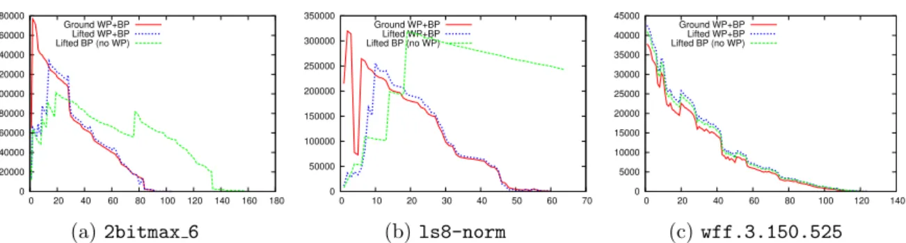
3.3 Results for Lifted Warning Propagation . . . 58
3.4 Illustration of Shortest-Path-Lifting . . . 62
3.5 Example Highlighting the Need for Iterative Shortest-Path-Lifting . . . 64
3.6 Experimental Results for Lifted Decimation . . . 68
3.7 Results for Lifted Belief Propagation Guided Sampling . . . 69
3.8 Illustration of a Mixture of Bayesian Networks . . . 72
3.9 Re-Lifting with Pseudo Evidence . . . 76
3.10 Mixture of Bayesian Networks for a Clamped Factor Graph . . . 77
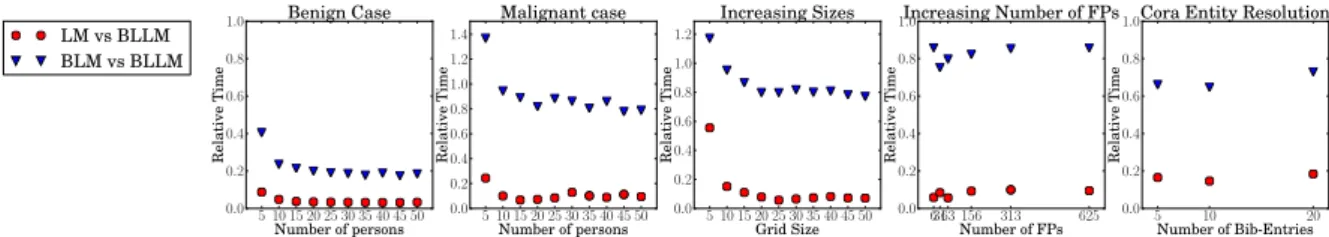
3.11 Run Time Comparison for BLLM . . . 81
3.12 Binary Image Segmentation with BLLM . . . 83
3.13 Example MRF Raising Decoding Issues in LM . . . 85
5.1 Running Example for Label Propagation . . . 101
5.2 Illustration of Lifted Label Propagation . . . 104
5.3 Example of a Fractional Automorphism . . . 105
5.5 Dataset Statistics for Online Bibliographies . . . 107
5.6 Worldwide Paper Count After Running Label Propagation . . . 108
6.1 Inferring Migration from the Web . . . 114
6.2 Illustration of Migration Propensities . . . 117
6.3 Migration Statistics over Time in GeoDBLP . . . 118
6.4 Migration Propensity Fit . . . 119
6.5 Migration Propensity on the Continental Level . . . 120
6.6 Migration Propensity on the National Level . . . 121
6.7 k-th Migration Propensities Fit . . . 122
6.8 Brain Drain and Inter-City Migration . . . 124
6.9 Running HITS and PageRank on the Migration Graph . . . 125
6.10 Markov Process for SIR Models . . . 130
7.1 Comparison Between Consistent and Local Count Models . . . 138
7.2 Illustration of a Poisson Dependency Network . . . 140
7.3 Example of a Log Link PDN with Multiplicative Updates . . . 147
7.4 Example of a Poisson Regression Tree . . . 148
7.5 PDNs Capturing Positive and Negative Dependencies . . . 152
7.6 PDNs Predicting Cell Counts . . . 154
7.7 Visualization of a PDN Representing the NIPS Text-Corpus . . . 158
7.8 Learning Rates for Individual Crimes . . . 159
7.9 Model Fit of PDNs on the Communities & Crime Dataset . . . 160
7.10 Illustration of Relational Count Databases . . . 161
1.1 Summary of Technical Chapters . . . 8
2.1 Formulas Used in the Smokers-and-Friends-MLN . . . 27
2.2 Formulas Used in the Smokers-and-Friends Dynamic MLN . . . 28
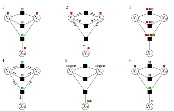
3.1 Exemplifying Belief Propagation on a CNF . . . 50
3.2 Experimental Results for Lifted Decimation . . . 67
3.3 Qualitative Results for BLLM on Synthetic Data . . . 82
3.4 Qualitative Results for BLLM on Entity Resolution . . . 84
5.1 Label Accuracy for the AAN Dataset . . . 103
6.1 Goodness-of-Fit for Migration Propensities . . . 119
6.2 Goodness-of-Fit for k-th Migration Propensities . . . 123
7.1 A Comparison of Poisson Graphical Models . . . 137
7.2 Experimental Results for PDNs on Network Discovery . . . 153
7.3 Training Quality of PDNs for Cell Counts and Publication Data . . . 156
1 Belief Propagation with Parallel Updates . . . 35
2 Color Passing as Proposed by Kersting et al. [114] . . . 37
3 Lifted Decimation . . . 57
4 Lifted Decimation Using SPS-Lifting . . . 66
5 Evidence Aware Color Passing . . . 78
6 Bootstrapped Lifted Likelihood Maximization . . . 79
7 Label Propagation as Proposed by Zhu and Ghahramani [260] . . . 92
8 Matrix Adaption Replacing Push-Back-Phase . . . 93
9 Learning Algorithm for Poisson Dependency Networks . . . 141
Introduction
Providing machines with some kind of intelligence and enabling them to operate in a smart manner has been a longstanding goal of mankind and the field of Artificial Intelligence (AI). We can clearly see that AI and also Machine Learning are affecting our everyday lives more and more, and their ample capabilities have just begun to have an impact. Until today, robotics has been widely recognized as the driving force behind AI and Machine Learning but there is a much wider range of applications that can and will benefit from these techniques: for instance those within the predominant era of Big Data. In this context, not only areas such as medicine and biology, but also whole branches of computer science like computer vision, natural language processing, and information retrieval, to name only a few, have been revolutionized by AI. This again has been facilitated by today’s mass storage capabilities which make storage fast and cheap. Besides these areas of research, we are starting to see many applications throughout the industry enjoying the great advantages of Machine Learning. Both, eCommerce and mobile commerce for instance, are increasingly depending on Machine Learning. Recommender systems, as a common and wide-spread example, help to objectify advertisement in these branches to leverage the effectiveness of newsletters and banners. The foundation of detecting latent patterns — for example in data of human behavior — in any of the aforementioned sciences and applications would not have been possible without the help of statistical learning.
Although a lot of progress has been made over the past decades, much remains to be done in the future if we are to reach the goals we all imagine — namely those of applying intelligent algorithms into a real-world context. Due to the low costs of data storage and computational power, many companies have started gathering tons of data. They are, however, unable to discover latent knowledge and information due to the missing expertise, which also prevents them from generating revenue from the available data. There seems to be an agreement that large amounts of data are a crucial key to AI. However, it still remains to be answered if Big Data is really the skeleton key to all AI problems. This is where Machine Learning is starting to play a fundamental role by learning descriptive models from data and to use the derived models to make predictions on unseen instances. Nevertheless, Big Data also poses new challenges for Machine Learning in terms of complexity. In many of these cases, we do not see a single instance in isolation but instead a set of objects all interacting with each other.
Often, several of these objects are of the same type, such as customers in databases throughout the retail industry. In these cases, we are interested in predicting characteristics of customers: for example their churn or buying behavior [157, 85, 204].
One crucial effect that is often present in these kind of situations isautocorrelation [102] which is the statistical dependence between such interacting entities or objects of the same type. Friends for example may share similar interests. If one person buys a specific item, it could be worthwhile recommending this item to their friends. Here, friendship as such implies a relational structure between objects, or database entries, and thereby introduces dependencies. This holds in many other situations and the data we observe on an everyday basis is inherently relational, making the common assumption in Machine Learning of identically and independently distributed instances not suitable. Instead, this type of data asks for collective classification and regression. Jensen et al. [103] discuss this issue in particular for relational probabilistic models and conclude that collective approaches can greatly reduce the error in prediction with comparable results to non-relational approaches in the absence of autocorrelation.
Modeling links, such as the aforementioned example of friendship, is a common pattern in relational databases which belong to the most widespread form of data storage representing structured information. The field of Inductive Logic Programming [44] is concerned with learning logical rules from such databases that hold throughout the entire knowledge base. It must be noted however that real-word data often underlies uncertainty which additionally makes modeling and learning far more complex. For example, intelligent customer relationship management and marketing databases wish to store uncertain information on customers such as churn and buyer conversion likelihoods. And again, we can assume that the decisions made by customers related to each other are not independent. Models describing relational data under uncertainty have become more popular than ever and this trend is also visible in the increasing usage of probabilistic databases [216]. Early work in this area already combined relational query languages with probabilistic models [221], allowing developers familiar with SQL to specify complex probabilistic models. However, accessible and fast inference in these problem settings is crucial for the applicability of such modern AI and Machine Learning approaches. A broader application of such technologies will hopefully not only facilitate further advances in AI and computer science in general, but also trigger new data storages that are capable of handling Big Data under uncertainty.
There is a wide a range of approaches and algorithms capable of learning from observations which also provide extensions that carry over to the relational or multivariate setting. One particular class of models that can learn from different types of data and represent general interactions between observations, are Probabilistic Graphical Models (PGMs). PGMs model the probability distribution of the observed data and allow to collectively infer missing values from the underlying joint distribution. The impact of PGMs on AI has been huge and has also been valued by the ACM recently by awarding Judea Pearl the Turing Award in 2011. Pearl’s work on Bayesian Networks, a subset of PGMs, and Belief Propagation, which is an inference algorithm within these models, commenced a new era within probabilistic reasoning. A significant part of the work at hand is also based on Belief Propagation and the idea of message passing for inference.
Large-scale databases with millions of customers comprise difficult challenges for learning and inference in PGMs with theoretical results limiting both in the exact case. Correspondingly, various approaches have been presented to make inference tractable. One, namely the exploita-tion of symmetries in the data, has been receiving a lot of attenexploita-tion in recent years. Its general
idea is to group indistinguishable objects together and to operate on the resulting clusters. Roughly speaking, this means that not every customer in a database is distinct in terms of the underlying problem and many customers exhibit the same characteristics. So, instead of making predictions on an individual level, we can now work on the clusters of customers. This can reduce the problem size by orders of magnitude and hence significantly reduce the required time for inference. In the Statistical Relational Learning (SRL) community, this approach is known aslifting orlifted inference. So far, lifted inference has been focusing on relational PGMs with mostly binary random variables and several of these lifted inference approaches are based on message passing. However, lifting is also useful in other settings and binary PGMs often limit the expressiveness or make statements overly complex. To further highlight these current limitations of PGMs and lifting, we now present three examples to motivate the contributions of this thesis.
1.1 Illustrating “non-standard” PGMs and Lifted Inference
Our focus is on PGMs and lifted inference approaches in “non-standard” settings. We will now provide three illustrative examples which will highlight our contributions and exemplify our understanding of these “non-standard” settings.
Lifted SAT — Lifted Message Passing Beyond Probabilistic Inference
One of AI’s key challenges in moving ahead is closing the gap between logical and statistical AI. While logical AI has mainly focused on complex representations of knowledge, statistical AI has concentrated on the aspects of uncertainty. However, intelligent agents and systems must be able to handle both, namely the complexity and the uncertainty of the surrounding real world. While extending relational data with probabilities has been pursued in many research areas, PGMs have become one of the most successful approaches to combine logic with probabilities and have greatly contributed to the recently emerging fields of SRL [66] and
Statistical Relational AI (StarAI)1 [116].
Lifted inference algorithms, exploiting the relational structure of models, have rendered large and previously intractable probabilistic inference problems quickly solvable. In these cases, the logical representation is merged into the PGM whereupon the probabilistic inference algorithm is applied. In this regard it is worthwhile asking if the idea of lifting is applicable to algorithms solving logical problems that operate on similar concepts as probabilistic inference algorithms. As the following example suggests:
lifted message passing is not limited to probabilistic inference algorithms.
And taking this one step further, we will now indicate how instances of theBoolean satisfiability problem (SAT) [193] can be solved more efficiently based on lifted inference, hence, connecting logical and statistical AI in a “non-standard” setting.
SAT is one of the well known NP-complete [41] problems and efficiently solving particular classes of SAT instances contributes in many ways. Problems from knowledge representation, planning, scheduling, model checking, and many more, can all be reduced to SAT. A SAT problem poses the question if a given formula in propositional logic evaluates to True. Here, we assume that the formula is given inconjunctive normal form (CNF), i.e., a conjunction of
1
1 2 3 4 2 ? ? ? 3 ? ? ? 4 ? ? ? (a) Problem 1 2 3 4 2 4 1 3 3 1 4 2 4 3 2 1 (b) Possible Solution
Figure 1.1: (a) Normalized Latin square of size four. Any solution fills the missing cells, denoted by a “?”, in such a way that each row and each column uses each number (color) exactly once. One possible solution is depicted in (b).
disjunctions. This assumption is very common and does not impose any restrictions, since any formula can be converted into CNF. A solution to a SAT problem is an assignment to variables such that the underlying Boolean formula evaluates to True. Similar to lifted inference in relational models, we can exploit symmetries in the structure of propositional formulas when solving SAT problems and thus solve the underlying problem more efficiently. However, in contrast to many relational lifted inference approaches, we tackle the problem from the opposite point of view and follow a bottom-up approach.
We will now give a concrete example of a SAT problem and indicate how it can be solved. Figure 1.1a shows an example of a Latin square2 which is akin to the popular Sudoku game. Similar to Sudoku, in a Latin square the goal is to label every unknown cell in such a way that each column and each row uses every number exactly once. In Figure 1.1a, this is further highlighted by using different colors for each number. The depicted example has a size of four with an additional constraint being that the first row and column are already labeled. Such a Latin square with a natural ordering in its first column and row is also called normalized3. We can now define a set of propositional clauses that describe the labeling problem more precisely based on the following constraints:
• Every cell is labeled with exactly one number.
• Every number occurs only once in every row.
• Every number occurs only once in every column.
Finding a solution to a Latin square can also be considered as finding a solution of a CNF respecting these specific constraints. Each variable in the CNF corresponds to the labeling of a specific cell with a particular color. While a normalized Latin square of size four has 21 variables, this number grows cubically with the size of the problem. Hence, one cannot simply try all combinations to find a solution to the problem we are trying to solve.
If we look at the formulas of a CNF representing a Latin square, we see that the clauses for each cell look similar and all cells are constraint likewise. As we will see below, this insight can be advantageous in iterative problem solving procedures which can be used to find solutions to SAT problems. This can be illustrated by representing the CNF as a graph which comes with the benefit of giving us a “neighborhood”-concept and hence some kind of relational information. To be more precise, we define the CNF by means of a factor graph (see Section 2.1.1 for a
2en.wikipedia.org/wiki/Latin_square 3
Other Latin squares with different constraints can be found at http://www.cs.ubc.ca/~hoos/SATLIB/
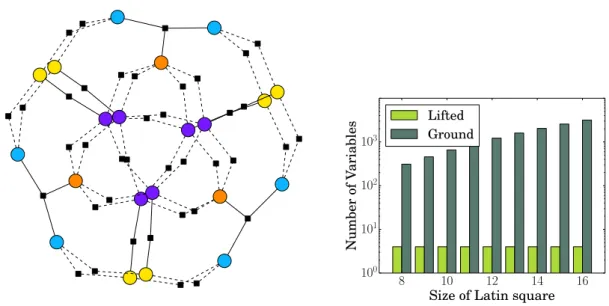
8 10 12 14 16 Size of Latin square 100 101 102 103 Number of Variables Lifted Ground
Figure 1.2: (left) Latin square of size four represented as a factor graph. The colors indicate clusters of variables that are constrained the same way. (right) Comparison of ground and lifted Latin squares for reasonable sizes. The ground problems grow cubically while the number of lifted variables remains constant.
detailed description of factor graphs). Figure 1.2(left) shows the factor graph representation for the Latin square of size four. Each variable is depicted as a circle and each square represents a clause. Each clause is connected to its variables via an edge. Dashed edges indicate that a variable appears negated in a clause.
Looking at the graph more closely, we see that the factor graph is symmetric and one can form different clusters of variables which are distinguished by colors. Note that these colors do not correspond to the colors which are used to color the Latin square itself in Figure 1.1. Symmetries in the factor graph arise from the fact that variables assigning the same label to different cells in the Latin square are constrained in the same way by the propositional formulas. An algorithm that finds such clusters based on sending messages in the graph will be explained in Section 2.4.1. For now, however, keep in mind that identically colored variables in the factor graph behave the same way. We will now indicate how the knowledge about these clusters speeds up the inference process.
Common approaches to solving SAT problems choose a variable heuristically, set its value to either True orFalse, simplify the CNF, and choose the next variable to clamp. Usually, the heuristic needs to be evaluated for each variable to make a locally optimal choice. Having a symmetric problem as the one described here, we can group the variables in such a way that we only have to evaluate the heuristic for each cluster because we know that each variable in a cluster behaves identically. For our current example, all variables in a cluster of the same color behave identically. Hence, we only need to apply the heuristic once to a single variable from this cluster.
This might not be impressive in the case of such a small problem. Therefore, let us have a look at Latin squares of increasing size. Figure 1.2(right) shows a comparison of ground and lifted Latin squares for realistic problem sizes. We see that the number of ground variables (dark green) increases cubically as stated above (note the log-scale of the plot). In contrast, the
Paper 1
Paper 2
Paper 3
Figure 1.3: Extract of an online bibliography enriched with geographic information. A node corresponds to an author-paper-pair and dotted boxes refer to a paper written by the enclosed authors. The labels reflect the geographic location of an author while having written the particular paper and edges connect either co-authors or nodes of the same author for different papers.
number of lifted variables (light green) remains constant which is quite remarkable. Nevertheless, this is a common observation made in the lifted inference literature. In the case of probabilistic inference, it is often observed that the ground run time grows exponentially while the lifted run time only increases polynomially with growing problem sizes. At this point we should also mention that the level of compression drastically decreases once we clamp variables and simplify the model. In the worst case, we can no longer lift the model after simplification and detecting clusters becomes an unnecessary overhead. This aligns with setting evidence in PGMs where lifted inference for the unconditioned probability is fast but with evidence being set, the potential for lifting decreases.
The concept of lifting will be used throughout various parts of this thesis and will be applied in new areas apart from probabilistic inference in relational PGMs. We will return to the problem oflifted satisfiability in Section 3.1 where we will discuss and evaluate different problem instances in greater detail. More specifically, we will show that lifted inference can speed up SAT solving but also asks for new algorithms exploiting symmetries efficiently when variables are clamped. In this context, we will also discuss the problem of clamping in detail and we will propose algorithms that are capable of exploiting symmetries after setting evidence (see Section 3.2 and Section 3.3).
Lifted Labeling — Label Propagation on Lifted Matrices
The first example showed how instances of logical problems contain symmetries and illustrated how these symmetries can be exploited during problem solving. The idea of coloring the CNF is tightly connected to the message passing algorithm that is used in the decimation framework. However, this computational view on lifting can also introduce additional complexity as it requires changes to the messages being sent around (see Chapter 3). When looking at other problems and algorithms, we will see that symmetries in the problem structure itself can be exploited in such a way that the inference algorithm remains unaffected. This way, lifting can be seen as a preprocessing step. In a nutshell, the underlying graph can be lifted by algebraic means and the inference procedure, a sequence of matrix-matrix-multiplications, remains unchanged but now uses lifted matrices. In contrast to much of the existing literature, we show that
lifting is not limited to binary variables and does not necessarily require the modifi-cation of the ground algorithm.
Figure 1.4: The prediction of traffic flows can be naturally realized by graphical models over count random variables. Dark red spots indicate a high traffic flow and the black arcs indicate how traffic segments influence each other.
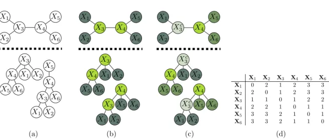
We will now explain this idea for a labeling task with possibly thousands of labels. Let us assume that we want to label entities in a database. For example, one is interested in labeling the authors in a bibliography with their affiliations while writing a particular paper. Figure 1.3 illustrates this idea for a small database extract. Here, each node corresponds to an author of a paper while country flags are used as an approximation to an author’s affiliation. Unknown affiliations are left blank. The dotted boxes enclose authors of the same paper. Each edge in the graph connects either two nodes corresponding to authors of the same paper, or two nodes of the same author but for different papers. The edges are supposed to model a similarity between nodes. Taking a closer glance, the presented graph encodes the intuition that neighboring nodes are more likely to share the same label. With this information we can now propagate the initial labels throughout this graph based on the edges. This is achieved by representing the graph and the initial labeling as matrices. Iteratively multiplying the label matrix with the similarity matrix results in a distribution over the labels for each node. This algorithm is known as Label Propagation [260].
In symmetric examples such as the one depicted in Figure 1.3, we can lift both of the involved matrices by algebraic operations returning two compressed datastructures. Interestingly, these lifted matrices can directly be used for the multiplications instead. The same label distribution as in the ground case can be read off the label matrix of reduced size. This idea of Lifted Label Propagation will be discussed in Section 5.3 in more detail. However, using a Gaussian similarity function, as it is often done, results in a dense similarity matrix, hence, limiting the applicability of Label Propagation in large-scale settings. Therefore, we resort in Section 5.1 to SRL concepts and define the similarity matrix based on logic formulas akin to relational PGMs.
Count Data — Graphical Models Beyond Multinomial and Gaussian Random Variables
The previous example has already shown a labeling task where the alphabet can be fairly large, albeit, still finite. In many other cases, we are confronted with variables defined over the natural numbers, i.e., discrete but infinite. Most of the existing PGMs are either multinomial or Gaussian, and thus ill-suited to represent the natural numbers appropriately in many situations.
Range Inference Learning Lifting Chapter 3 {0,1} BP, SP, WP, LM max. LL Color Passing Chapter 5 {0, . . . , d} LP min. entropy saucy
Chapter 7 N MCMC max. LL via GTB ongoing work
Table 1.1: This thesis covers different types of probabilistic graphical models and algorithms along with it. This table gives a brief overview on the approaches used in each technical chapter.
Extending PGMs to variables defined over the natural numbers is necessary to represent a large class of problems adequately.
To underline the necessity and benefits of such models, let us present a new example from the domain of traffic flow prediction. Figure 1.4 shows a map extract displaying the vehicular traffic from 38 stationary detectors located on the Cologne orbital freeway stretch adding up to 50 km in Germany. Each detector counts the number of cars passing by per minute and is naturally represented as a count random variable. Here, dark red detectors indicate high traffic and possibly a network congestion. An observation of the entire network for a certain point in time can be seen as one sample from a joint probability distribution of count random variables. Modeling this distribution requires to learn the dependencies between individual traffic segments.
Existing PGM approaches to such problems either discretize the count data into bins or follow a Gaussian approximation. Both techniques solely approximate the true nature of the counts. We therefore introduce in Chapter 7 a new class of PGMs based on Poisson distributions. These
Poisson Dependency Networks (PDNs) are capable of learning dependencies between count random variables and inference in these models is based on a simple sampling procedure.
The black edges in Figure 1.4 feature the dependencies between detectors learned by a PDN. One can easily see that the dependencies of a highway segment do not solely depend on neighboring segments close by, but also on critical highway segments in other regions. Besides describing the traffic flow in the network, we can now also make predictions for missing datapoints or future situations. For example, detectors may often fail due to technical issues or construction sites. When these detectors are offline, we can use PDNs to fill in the missing counts. The ideas of modeling traffic based on counts has been further pursued in [96] and within the collaborative research center SFB 876, project B44.
1.2 Outline and Summary of Contributions
This thesis makes several contributions to inference and learning in PGMs by applying ideas from relational PGMs and lifted inference to non-standard settings. The examples in the previous section have already illustrated our understanding of non-standard settings and we will now summarize the content of this thesis in greater detail. Table 1.1 gives an overview how the models in the main technical chapters differ and how different inference and learning approaches are used accordingly. As we have seen in the previous three examples and as it is further shown in Table 1.1, the main technical chapters focus on random variables with different ranges, i.e., binary, multiclass, or count random variables. Depending on the range of
4
the variables, different inference and learning approaches will be used in each chapter. The idea of lifting is a recurring concept and will be discussed for each case. The content and contributions of Chapters 2 to 7 can be summarized as follows:
Chapter 2 To prepare the ground for what is to follow, Chapter 2 gives an overview on PGMs, including inference and learning algorithms. Chapter 2 furthermore explains the idea of lifted inference in detail because the specific contributions of Chapter 3 rely on the idea of lifted message passing. In this context, Chapter 2 explains probabilistic inference based on message passing and describes one of the most prominent lifted message passing algorithms in detail. This chapter will also comment on more advanced lifting techniques, such as informed Lifted Belief Propagation published in:
K. Kersting, Y. El Massaoudi, B. Ahmadi, and F. Hadiji. Informed Lifting for Message-Passing. InProceedings of the 24th AAAI Conference on Artificial Intelligence (AAAI), 2010.
Since much of the lifted inference literature focuses on relational PGMs, Chapter 2 will also summarize the most well known formalisms in this area.
Chapter 3 While much of the early literature on lifted inference was primarily focusing on lifted variants of Variable Elimination and Belief Propagation, Chapter 3 introduces lifted versions of message passing algorithms beyond lifted Belief Propagation. We extend the understanding of lifting by introducing additional lifted versions of existing inference algorithms including Warning Propagation and Survey Propagation. Warning Propagation and Survey Propagation are message passing algorithms used to solve SAT problems; the lifted counterparts were published in:
F. Hadiji, K. Kersting, and B. Ahmadi. Lifted message passing for satisfiability. InWorking Notes of the AAAI Workshop on Statistical Relational AI (StarAI), 2010.
As the introductory examples in the previous section already indicated, lifting is most effective in the unconditioned case, i.e., when no evidence is given or no variable has been clamped yet. However, iterative approaches to solving SAT instances clamp one or more variables in every iteration and therefore ask for lifting algorithms that can efficiently handle incremental evidence. To this end, we introduce a framework that is fitted to such sequential clamping approaches. This framework was previously published in:
F. Hadiji, B. Ahmadi, and K. Kersting. Efficient Sequential Clamping for Lifted Message Passing. In Proceedings of the 34th Annual German Conference on Artificial Intelligence (KI), 2011.
In particular, the proposed decimation approach tries to lift a clamped model more efficiently by adapting the unconditioned lifted model. To do so, it makes use of additional information from the network structure in form of shortest path distances. This Shortest-Path-Sequences lifting has been published in:
B. Ahmadi, K. Kersting, andF. Hadiji. Lifted Belief Propagation: Pairwise Marginals and Beyond. In Proceedings of the 5th European Workshop on Probabilistic Graphical Models (PGM), 2010.
Message passing algorithms as such work in an iterative way by exchanging messages to optimize an algorithm-specific criterion. In certain cases, this optimization obeys a
monotonic behavior which can be interpreted as a process approaching evidence. We cut this process short and set the evidence during the message passing already, before the algorithm has completely converged. We show that such a likelihood maximization algorithm is liftable, yet requires a new lifting approach to handle the new evidence during the message passing itself. The lifted version of this maximum a posteriori inference algorithm together with the adapted lifting algorithm was published in:
F. Hadiji and K. Kersting. Reduce and Re-Lift: Bootstrapped Lifted Likeli-hood Maximization for MAP. In Proceedings of the 27th AAAI Conference on Artificial Intelligence (AAAI), 2013.
Combining these contributions, we extend the applicability of lifting to new areas and establish lifting in these settings as a novel approach to reduce run time. We furthermore propose new lifting schemes that cope with incrementally growing sets of evidence to exploit symmetries even more effectively.
Chapter 4 The algorithms in Chapter 3 are based on message passing. When lifting these algorithms, the ground message passing algorithms have to be modified to respect the lifted model. Chapter 4 presents an alternative view on probabilistic inference without message passing. Instead, it reviews the well known semi-supervised Label Propagation algorithm. Label Propagation is used to label a graph based on a matrix representation of the similarity between nodes and a set of initially known labels. This algorithm features a probabilistic interpretation as well and returns a distribution over labels for each node in the graph. While Chapter 3 handles binary PGMs only, Label Propagation can naturally process large label alphabets and hence solve multiclass labeling problems. In the next step, we review connections between graph theory and lifted probabilistic inference that have been established recently, to ultimately motivate a lifted version of Label Propagation in the subsequent chapter.
Chapter 5 Standard Label Propagation commonly uses a Gaussian function to model the similarity between nodes. This results in a dense similarity matrix which does not scale to large graphs with millions of nodes. Relational PGMs have been shown to easily describe dependencies between related objects by using first-order logic as a template language. We apply these ideas to Label Propagation and define similarity matrices based on weighted logical rules. Such a rule-based approach for Label Propagation entails several advantages. First, logical rules allow an intuitive problem definition as knowledge can be encoded more easily with the help of domain experts. Second, logical rules often lead to much sparser similarity matrices compared to the standard setting where a Gaussian function is used. As our empirical results show, this relational Label Propagation still produces high accuracy labels. At this point, one may reflect upon whether Label Propagation is liftable too, especially when using a rule-based similarity function. In this regard we show that the interplay of graph theory and lifting algorithms can be applied to Label Propagation and we prove that Label Propagation can be lifted in terms of algebraic operations; the Lifted Label Propagation algorithm has recently been accepted in:
F. Hadiji, M. Mladenov, C. Bauckhage, and K. Kersting. Computer Science on the Move: Inferring Migration Regularities from the Web via Compressed Label Propagation. In Proceedings of the 24th International Joint Conference on Artificial Intelligence (IJCAI), 2015.
Lifted Label Propagation results in a much faster labeling algorithm with less memory consumption. Furthermore, lifting becomes a single pre-processing step that does not require modifying the ground version. Hence, Lifted Label Propagation can be combined with any other method making Label Propagation more efficient.
Chapter 6 In Chapter 5, we use lifted relational Label Propagation to label large-scale online bibliographies with geographical attributes. Starting with a freely available online bibliography, we harvest additional information from the Web to add initial seed affiliation of authors to our database. Label Propagation is then used to fill in the missing affiliation information, resulting in a database of several million papers and authors augmented with geographical tags. Having such a vast resource at hand, Chapter 6 will point out that several interesting patterns and regularities can be found in this dataset. We show how to derive several statistical regularities and patterns from these geo-augmented bibliographies by fitting simple distributions to the data based on the maximum likelihood estimation principle. Our findings encompass distributions describing the migration behavior of researchers, as well as a general model for the academic job market. Excerpts of these patterns and regularities have been included in the IJCAI-15 publication referred to above and a full analysis has been made publicly available at:
F. Hadiji, K. Kersting, C. Bauckhage, and B. Ahmadi. GeoDBLP: Geo-Tagging DBLP for Mining the Sociology of Computer Science. arXiv preprint arXiv:1304.7984, 2013.
Such an analysis of human behavior is applicable to various other kinds of datasets and we further highlight how we have used such techniques to describe the attention to Internet memes [14] and the spread of viral videos [15].
Chapter 7 While Chapter 3 focuses on binary variables and Chapter 5 deals with multiclass problems, Chapter 6 furthermore highlights that we are still missing the setting with variables defined over infinite ranges. This gap is filled in Chapter 7 where we take a closer look at random variables defined over the natural numbers and count data in general. While Chapter 6 fits distribution to count data for descriptive purposes, Chapter 7 presents models that allow a prediction conditioned on observations. Although counting is key to describing various observations and statistics, there is little work on PGMs for random variables defined over the natural numbers so far. We therefore introduce a different class of PGMs, namelyPoisson Dependency Networks (PDNs), that is tailored towards count data based on Poisson distributions, as previously existing graphical models were mainly focusing on discrete and finite data or Gaussian random variables. Although PDNs consist of a set of local conditional Poisson distributions, we show how to sample from the joint distribution with the help of a Gibbs sampler. Besides answering probabilistic queries, these samples can also be used to predict counts of unseen instances. In order to efficiently learn PDNs, we resort toGradient Tree Boosting (GTB). GTB has successfully been used in a large variety of applications where a stepwise optimization is performed by summing together the output of simple basis functions. Besides the additive case, which relies on a step-size specified by the user, we also present the first approach to multiplicative GTB to improve convergence. This multiplicative GTB shows to be an effective alternative in many cases that does not require the tuning of a step-size. This new class of PGMs has recently been published in:
F. Hadiji, A. Molina, S. Natarajan, and K. Kersting. Poisson Dependency Networks: Gradient Boosted Models for Multivariate Count Data. Machine Learning Journal, 2015.
We further touch upon relational extensions for this model class and also describe how lifting could be implemented to motivate future work in this area.
We conclude in Chapter 8 by summarizing the main aspects of this thesis, presenting the lessons learned during the development of this thesis, and suggesting possible directions for future work. A list of selected publications in which the author was involved can be found in Section 1 of the Appendix which also details the author’s specific contributions to each paper.
The reader may notice that the chapters are not equally dense. In particular, Chapter 3 is comparably more extensive. This primarily rises from the fact that much of this thesis was motivated by the initial work on lifting as described in Chapter 3. The work therein started to look at lifting in “non-standard” settings, however, still focusing on message passing algorithms in binary PGMs. While this work evolved, many of the ideas presented in Chapters 4 to 7 were developed, extending PGMs and ideas from lifting by additional dimensions. Therefore, we propose as a future research question to investigate lifting in the probabilistic count models presented in Chapter 7 which in combination would once again emphasize the core contributions of this thesis.
From Probabilistic Inference to Lifted Message Passing
There are a couple of definitions and ideas that return in each of the following chapters and will be summarized in the current chapter. This mainly focuses on the definition of PGMs and particular instantiations of this formalism. It also includes the main challenges in PGMs and state-of-the-art approaches for solving them. A discussion on inference and learning in PGMs requires basic ideas from probability theory. Similarly, relational PGMs depend on terminology from logic. We will now describe these ideas and concepts in greater detail.
2.1 Probabilistic Graphical Models
In this section, we give a short introduction to PGMs and define our notation. For a more detailed review of PGMs, we refer the interested reader to [124, 237]. Generally, PGMs combine ideas from graph theory and probability theory. Let us assume that we are given a graph G = (V, E) where V ={V1, V2, . . . , Vn} is a set of vertices and E ⊆V ×V is a set of edges.
Each edge eij connects two vertices Vi, Vj ∈ V. In the most general form, we consider undirected edges between the nodes. In order to define a PGM, we further assume that we have a random variable Xi associated with every vertex Vi ∈V. Each variableXi is defined over a range Xi. Throughout this thesis we will consider different ranges, starting from binary ones, e.g.,Xi ={0,1}, over discrete but finite ones, e.g., Xi={0,1, . . . , d}, to discrete and infinite ones, e.g., Xi =N. We will also touch upon continuous ranges along the way, i.e., Xi =R+,
because the Gaussian setting for instance is related to the discrete case in many ways and various concepts carry over. Letxi represent a possible instantiation of random variableXi, i.e., xi ∈ Xi. We define a vector of nrandom variables as X= (X1, X2, . . . , Xn) andxas its instantiation. We now associate apotential function orcompatibility function φcwith every cliquec of the graphG. A clique is a fully connected subset of vertices inGand we define the set of all cliques inG asC. By Xc, we refer to the variables contained in cliquec. Based on these potential functions, we can formulate the following factorization of a joint probability distribution: p(X=x) = 1 Z Y c∈C φc(xc). (2.1)
X1 X2 X3 (a) Example MRF X1 X2 X3 (b) Example BN X1 X2 X3 (c) Example DN
Figure 2.1: A visual comparison of the different probabilistic graphical models that are covered in this thesis.
Here, each function φc is a non-negative function over a subset of the variables Xc, i.e., φc : X1 ×. . .× X|xc| → R
+. Z = P
x∈X1×...×Xn
Q
c∈Cφc(xc) is a normalization constant, ensuring that p(·) is a valid probability distribution. The product of positive functions, or possibly even local probability distributions, in Equation (2.1) together with a graph defines what is known as a Markov Random Field (MRF). A small example MRF is depicted in Figure 2.1a. This relationship between a graph and a probability distribution goes back to the theorem of Hammersley-Clifford [89, 19]. The theorem of Hammersley-Clifford states that we can find such a factorization over cliques for every positive probability distribution, i.e., where we have∀x:p(X=x)>0. This highlights the great expressiveness of MRFs and gives the theoretical foundations. Furthermore, the factorization of the graph describes the conditional independencies of the distribution. By this, the graphG, or equivalently the MRF, tells us that variable Xi is independent of all other variables in the graph given its direct neighbors nb(i), i.e., P(xi|x\i) =P(xi|nb(i)). Here, x\i refers to a random vectorx with variableXi removed. This is the so calledlocal Markov-property and Xi’s neighbors are also called Markov blanket. It is important to note thatC does not have to be the set of maximal cliques because any set of non-maximal cliques can be converted to a set of maximal cliques. Additionally, we also consider a single node as a clique which often simplifies the model specification. In fact, every MRF can be equally represented by a pairwise MRF, i.e., a model with pairwise potential functions only. We also want to note that the distribution in Equation (2.1) can be equivalently represented as a log-linear model:
p(X=x) = 1 Z Y c exp(wc·gc(xc)) = 1 Z exp " X c wc·gc(xc) # , (2.2)
where the features gc(·) are arbitrary functions over (a subset of) the configurationx andwc is a feature weight. We will come back to this model below where we describe MRFs based on weighted logical rules (see Section 2.3.1). In these cases, each gc corresponds to a function returning the truth value of a logical rule and wc defines its weight.
Using yet another reformulation of the MRF definition, we obtain aGibbs distribution which is often used in statistical Physics:
p(X=x) = 1 Z exp " −X c Ec(xc) # = 1 Ze − E(x), (2.3)
whereE(xc)>0 is the energy associated with the variables in cliquec. By settingEc(xc) =
−ln(φc(xc)), we obtain again our original form of the MRF. Energy-based formulations become interesting when one seeks for the most likely configuration of the distribution because maximizing the probability now equals minimizing the total energy.
We have now seen different representations of MRFs which all assumed some kind of potential functions, or more specifically in case of the log-linear representation, the MRF was based on feature functions gc and the corresponding weights wc(a.k.a canonical parameters). However, as we will see next, we can also parameterize the MRF in a different way. One can also view the distribution defined by the factorization in terms of a mean parameterization which is immediately related to the inference problems introduced in Section 2.2. We can define for each φca mean parameter E[φc(Xc)] =Pxcφc(xc)p(xc) which is then used to define a vector
of mean parameters over all potential functions (E[φ1(X1)], . . . ,E[φ|C|(X|C|)]). We can now
also define the set of all realizable mean parameters as:
M= ( τ ∈R|C||τ = X x φ(x)p(x) for some p(x)≥0, X x p(x) = 1 ) .
Here,φ= (φc, c∈C)∈R|C| is the vector of all potential functions andM defines a convex
polytope. We can assume without loss of generality that an MRF is pairwise, i.e., it contains only unary and pairwise feature functions. A procedure that transforms MRFs of arbitrary arity to a pairwise form is given in [237, E.3]. For such a pairwise MRF overG= (V, E), the mean parameters correspond to the marginal probabilities p(Xi) and p(Xi, Xj) for connected variables. In this case, we have
M(G) =
n
τ ∈R|C|| ∃p s.t. τi =p(xi)∀i∈V andτij =p(xi, xj)∀(i, j)∈E
o
, (2.4)
and refer to M(G) as themarginal polytope. These marginals, and marginals over any subsets of variables, are of great interest because one often wants to answer probabilistic queries in the form ofp(Xa=xa). Unfortunately, the number of constraints required to describeM(G) grows exponentially and therefore obtaining the mean parameterization efficiently is not possible in most cases. Indeed, determining the mean parameterization from the canonical representation amounts to probabilistic inference and is one of the main challenges in PGMs. The mapping in the opposite direction has an interesting interpretation as well and can be seen as parameter learning [237]. To reduce the number of required constraints, and hence the complexity, linear program relaxations have been proposed that focus on local constraints only. In particular, with the constraints
X xi τi= 1∀i∈V , X xj τij =τi, X xi τij =τj ∀(i, j)∈E , (2.5)
we can define thelocal marginal polytope
ML(G) =
n
τ ∈R|C||Conditions of Equation (2.5) hold.
o
,
which outer bounds M(G). But more importantly, ML(G) requires only a linear number of constraints in the number of edges. The marginal poltytopes M(G) and ML(G) will be of greater interest in Section 3.3 where we will refer to an algorithm that adds additional constraints to the polytope, in order to implement a fast approximate inference algorithm. For more information on the mean parameterization and the marginal ploytope, we refer to [237, Section 3.4].
Besides the undirected MRFs, there is another very popular class of PGMs, namelyBayesian networks (BNs) [124]. Here, the joint probability distribution is represented by means of a
directed, acyclic graph. Again, there is a node in the graph associated with each variable in the probability distribution. However, due to the fact that the graph is directed, we now have a set of parents for each node, referred to pa(Xi), instead of a Markov blanket as in MRFs. Each variable Xi is conditionally independent of its non-descendants in the network given its parents. This means that the marginal conditional probability distribution of each variable is specified by a probability table over the variable itself and its parents. The joint distribution of a BN is then defined as:
p(x) = n
Y
i=1
p(Xi|pa(Xi)). (2.6)
We saw for undirected models that the theorem by Hammersley and Clifford established the connection between an undirected graph and a probability distribution. Similarly, we have for BNs the representation theorem [124, Theorem 3.1 and 3.2] that connects a directed, acyclic graph with the factorization in Equation (2.6). An example of a BN is depicted in Figure 2.1b. Looking again at Equation (2.1), we can construct an MRF based on the conditional probability tables of an BN. We represent each conditional probabilityp(Xi|pa(Xi)) by a potential function over Xi∪pa(Xi), resulting in Z = 1. However, the structure of the MRF is not identical to the BN’s graph, as we have to connect all parents of a node. This conversion is often referred to as moralization and the resulting graph is called a moral graph. For example, if we moralize the BN in Figure 2.1b, we obtain the undirected model in Figure 2.1a which is completely connected. This example already highlights that we lose some of the independence information when transforming a BN into an MRF. The nodes X1 and X2 are marginally independent, however, it is not possible anymore to read off this information from the completely connected MRF. For more information on the connection between BNs and MRFs, as well as the encoded independencies, we refer the reader to [124, Section 4.5]. Nevertheless, every probability distribution defined by a BN can be encoded as an MRF as well.
Although BNs already impose restrictions on the graphical structure of the problems compared to MRFs, parameter and structure learning is still a tough challenge. Hence, models were proposed that combine advantages of both models but fail to define a consistent probability distributions in closed form. Nevertheless, these models still perform well on various tasks and reduce complexity of learning and inference significantly. One example of such models are
Dependency Networks (DNs) [90] which we find in between BNs and MRFs. DNs are defined as a set of local conditional probabilities that may contain cycles where each local conditional probability distribution is learned independently. An example of a DN is depicted in Figure 2.1c. We will describe DNs in larger detail in Chapter 7, as these models play a central role for our approach of handling count data, i.e., random variables over the natural numbers. Chapters 3 and 5 are mainly concerned with MRFs, although the work in Section 3.3 is solving the inference problem by transforming the original MRF into a mixture of simple BNs. While Chapter 3 is mainly concerned with binary MRFs, Chapter 5 looks at multinomial MRFs which however have an equivalent Gaussian representation in the case of binary variables.
As we have seen above, we can use graphs to formulate BNs, MRFs, and DNs. However, in many cases a different type of graph is more expressive as we will see next. This formalism, called factor graph, can represent all three types of models and hence factor graphs represent the main formalism to visualize graphical models in this thesis.
f1
X1 f X2
2
f3
X3
Figure 2.2: Example factor graph. Circles denote variable nodes and squares denote factors.
2.1.1 Factor Graphs
As we have seen in the previous section, there are different ways of defining graphical models. MRFs are represented by undirected graphs, while directed graphs are used for BN. However, there is also a formalism that is capable of representing both types of models, namely factor graphs [128]. Hence, factor graphs present an important formalism in this work, as several of our problems can be formulated in a unified way. Additionally, the factor graph formalism is more expressive than undirected graphs, since it can distinguish between pairwise and higher-order interactions. In a undirected graph, cliques of size two cannot be distinguished from cliques of size three. For example, the MRF shown in Figure 2.1a could very well represent a pairwise factorization p(x) = φ1(x1, x2)φ2(x1, x3)φ3(x2, x3), as well as a single clique φ1(x1, x2, x3). However, this circumstance would not be visualized appropriately with the corresponding underlying graph. More formally, a factor graph is a bipartite graphG= (V, E) that expresses the factorization of a joint probability distribution for p(X) as in Equation (2.1). Here, V is the set of nodes, which contains a variable node for each variableXi∈Xand a factor node for each φc∈C. There is an edge (i, c)∈E between the variable node forXi and the factor node corresponding to φc if and only if the variable is in the range of the function associated with the factor. SinceG is bipartite, there are no edges connecting two variable nodes or two factor nodes. In our figures, we will be denoting variables nodes as circles and factor nodes as squares. An example of a factor graph is depicted in Figure 2.2. Additionally, factor graphs also provide a probabilistic view on CNFs as we have seen in Figure 1.2: the marginals of the variables in a factor graph representing a CNF give the probability of the variable being True, respectively
False, when all solutions to the problem in Gare chosen uniformly, i.e., unweighted.
2.2 Inference and Learning in Graphical Models
This thesis covers different facets of inference and learning in PGMs. Therefore, we will now summarize the main challenges in this area. Assuming that the structure of a PGM and its parameters are already given, we are facing different inference tasks in order to answer probabilistic queries. However, in other settings we are starting solely with a dataset of empirical observations for which we first need to learn an appropriate PGM. Resulting form these different scenarios, we distinguish the following main challenges:
• Probabilistic Inference: Answering probabilistic queries for one or more variables is referred to as probabilistic inference. We can further split probabilistic inference into the following two subclasses:
– Marginal Inference: In many situations, we are interested in the marginal probability of a single node p(Xi =xi) =Z−1
P
x\i
Q
cφc(xc). In other cases, we might also need the probabilities of a subset of variables, i.e., p(Xc=xc), or the probability of an entire joint configuration p(X =x). Depending on the algorithm, different of these quantities are provided or can be read-off easily. In the case of BNs, the joint probability can be determined easily, while this requires the computation of the normalization constant Z in MRFs. For BNs we haveZ = 1. As seen above, Z is defined as the sum over exponentially many configurations which already indicates the hardness of its computation. Indeed, it can be shown that exact inference, i.e., the decision problemP(Xi=xi)>0, is NP-complete [124]. The proof follows a reduction from the 3-SAT problem which is known to be NP-complete. In correspondence to this results, it can also be shown that computing the marginal probabilityP(Xi =xi) itself is #P-complete [191]. Here, the proof follows a reduction from the model counting problem for 3-SAT. It can also be shown that probabilistic inference amounts to weighted model counting [34] which gives yet another connection to SAT related problems and their weighted extensions. Due to the hardness of inference in general, one often resorts to approximate inference algorithms. Parameter learning typically relies on computing the marginal probabilities and hence, efficient learning is also most often done in an approximate fashion.
– MAP inference: In other cases, we are not interested in the exact probability of a configuration but instead want to find the most likely one. The maximum a posteriori (MAP) inference amounts to finding the most probable assignment x∗
to all unobserved variables, i.e., the mode of the possibly conditioned distribution. More formally, the task of MAP inference is defined as
x∗ = arg max
x
p(x).
In general, this problem is NP-complete [203] as well. Still, MAP inference is a challenging and crucial task in solving different problems and it has applications in various domains such as image processing [251], entity resolution [206], and dependency parsing [144], among others. Here, the MAP assignment presents a solution to a specific problem and one is also required to use approximation algorithms in most situations. Important for MAP inference is the notion of max-marginals
which are defined as follows:
m(xi) = max
{x|xi=xi}
p(x) (2.7)
Many algorithms solve the MAP inference problem by calculating the max-marginals first. Having the max-marginals, one can decode the MAP configuration under certain assumptions [124, Section 13.1]. To be more precise, if each variable Xi achieves a unique max-marginalx∗i = arg maxxi∈Xim(xi), i.e., is unambiguous, then
equally be formulated based on an energy function (see Equation (2.3)). Therefore, the problem of MAP inference can equally be formulated as energy minimization:
arg max x p(x) = arg max x lnp(x) = arg min x − lnp(x) = arg min x ln(Z) +E(x) = arg min x E (x).
We can drop the normalization constant ln(Z) because we are just interested in a minimizing configuration. Moving to the log-domain has several advantages, e.g., we can avoid numerical instabilities of the multiplication and so on.
• Learning: We can further decompose the general learning task into two subclasses:
– Parameter Learning: Given an MRF, we are required to choose the potential functions or parameters, e.g., the weights wc in Equation (2.2). In generative
learning, one typically uses a training dataset and obtains the optimal parameter values by maximizing the log-likelihood over this training dataset. This approach is called maximum likelihood estimation (MLE)and assumes in the most simple case a fully observed dataset. Often, this already requires several calls to an inference procedure which highlights the importance of efficient marginal inference. For efficiency reasons, one often optimizes the pseudo-log-likelihood [20] instead of the true log-likelihood. In several situations, we can split the variables X of an MRF in observed and latent variables, i.e., variables that are always given (E) and variables that will be predicted based on the observed ones (Y). Here, we can use
discriminative learning that optimizes only the conditional log-likelihood p(Y|E) instead of p(X). A more detailed discussion of generative and discriminative models can be found in [217]. In Chapter 7, we will learn the parameters of conditional probability distributions and touch upon the issue of parameter learning in greater detail. MLE is typically done in supervised learning, however, in some situations, we are only given one mega-example which is additionally not fully labeled. We find ourselves in such a situation in Chapter 5 where we use an semi-supervised algorithm to solve a graph labeling problem. In this case, learning can be done via entropy minimization instead of MLE, as we will describe in Section 5.5. This combines the knowledge of known labels and the structure of the entire problem, however, it also introduces the assumption that parameters leading to low entropy are desirable.
– Structure Learning: The most challenging problem is structure learning because it also subsumes parameter learning as a subroutine. Here, we start solely with a given dataset and do not know the structure of the MRF in advance. Many structure learning algorithms start with an empty network or a network consisting of trivial potentials. In an iterative procedure, the existing potentials are refined or new potentials are generated based on the existing ones. A score function determines which new potentials are added to the model. Once the refinement process cannot improve the model anymore, the learning algorithm stops. Due to its high complexity, structure learning is often neglected and a structure is proposed in joint work with domain experts. With an exception in Chapter 7, we assume a given structure as well. The models proposed in Chapter 7 suggest a simple and efficient local learning