UC3M Working Papers Statistics and Econometrics 17-18
ISSN 2387-0303 November 2017
Departamento de Estadística Universidad Carlos III de Madrid Calle Madrid, 126 28903 Getafe (Spain) Fax (34) 91 624-98-48
Modeling and forecasting the oil volatility index
Massimo B. Maritia, João H. Gonçalves Mazzeub, Helena Veigac
Abstract _______________________________________________________________
This paper models and forecasts the crude oil ETF volatility index (OVX). The motivation lies on the evidence that the OVX has been used in the last years as an important alternative measure to track and analyze the volatility of future oil prices. The analysis of the OVX suggests that it presents similar features to those of the daily market volatility index. The main characteristic is the long range dependence that is modeled either by autoregressive fractional integrated moving averaging (ARFIMA) models or by heterogeneous autoregressive (HAR) specifications. Regarding the latter family of models, we first propose extensions of the HAR model that are based on the net and scale measures of oil prices changes. The aim is to improve the HAR model by including predictors that better capture the impact of oil price changes on the economy. Second, we test the forecasting performance of the new proposals and benchmarks with the model confidence set (MCS) and the Generalized-AutoContouR (G-ACR) tests in terms of point forecasts and density forecasting, respectively. Our main findings are as follows: the new asymmetric proposals have superior predictive ability than the heterogeneous autoregressive leverage (HARL) model under two known loss functions. Regarding density forecasting, the best model is the one that includes the scale measure as a proxy of oil price changes and considers a flexible distribution for the errors.
_______________________________________________________________________ JEL-Classifications: Q40; C51; C52; C53
Keywords: Forecasting OVX; Heterogeneous autoregression; Leverage; Net oil price changes; OVX; Scale oil price changes
a University Milano-Bicocca, Italy.
b Department of Statistics, Universidad Carlos III de Madrid, Spain.
c Universidad Carlos III de Madrid (Department of Statistics and Instituto Flores de Lemus), Spain and
BRU-IUL, Instituto Universitário de Lisboa, Portugal. Email: [email protected]. Corresponding author.
Acknowledgements: The third author acknowledges financial support from Spanish Ministry of Economy and Competitiveness, research projects ECO2015-70331-C2-2-R and ECO2015-65701-P and from Fundação para a Ciência e a Tecnologia, grant UID/GES/00315/2013.
Modeling and forecasting the oil volatility index
∗
Massimo B. Mariti
†Jo˜
ao H. Gon¸calves Mazzeu
‡Helena Veiga
§ABSTRACT
This paper models and forecasts the crude oil ETF volatility index (OVX). The moti-vation lies on the evidence that the OVX has been used in the last years as an important alternative measure to track and analyze the volatility of future oil prices. The analysis of the OVX suggests that it presents similar features to those of the daily market volatility index. The main characteristic is the long range dependence that is modeled either by autoregressive fractional integrated moving averaging (ARFIMA) models or by heteroge-neous autoregressive (HAR) specifications. Regarding the latter family of models, we first propose extensions of the HAR model that are based on the net and scale measures of oil prices changes. The aim is to improve the HAR model by including predictors that better capture the impact of oil price changes on the economy. Second, we test the forecasting performance of the new proposals and benchmarks with the model confidence set (MCS) and the Generalized-AutoContouR (G-ACR) tests in terms of point forecasts and density forecasting, respectively. Our main findings are as follows: the new asymmetric propos-als have superior predictive ability than the heterogeneous autoregressive leverage (HARL) model under two known loss functions. Regarding density forecasting, the best model is the one that includes the scale measure as a proxy of oil price changes and considers a flexible distribution for the errors.
JEL-Classifications: Q40; C51; C52; C53
Keywords: Forecasting OVX; Heterogeneous autoregression; Leverage; Net oil price changes; OVX; Scale oil price changes
1. Introduction
The price of oil has been fluctuating strongly in the last decade. It reached its maximum price in July 2008 to deplume to the value of $30.28 per barrel some months later. In the last seven years the oil crude barrel has been ranging from $125 to $30. These oil price fluctuations increase
∗The third author acknowledges financial support from Spanish Ministry of Economy and Competitiveness, re-search projects ECO2015-70331-C2-2-R and ECO2015-65701-P and from Funda¸c˜ao para a Ciˆencia e a Tecnologia, grant UID/GES/00315/2013.
†University Milano-Bicocca, Italy.
‡Department of Statistics, Univeridad Carlos III de Madrid, Spain.
§Universidad Carlos III de Madrid (Department of Statistics and Instituto Flores de Lemus), Spain and BRU-IUL, Instituto Universit´ario de Lisboa, Portugal. Email: [email protected]. Corresponding author.
oil volatility, and consequently, the risk exposure of both companies dedicated to exploring and processing oil, and investors.
The Chicago Board Option Exchange (CBOE) calculates and reports the crude oil ETF volatility index since May 2007. The index, according to CBOE, “measures the market’s ex-pectation of 30-day volatility of crude oil prices and it is calculated using the market volatility index (VIX) methodology for the United States Oil Fund”.1 OVX uses real-time bid/ask quotes
of nearby and second nearby options with at least eight days to expiration, and weights these options to derive a constant, 30-day measure of expected volatility. According to Chen et al. (2015), OVX is a way to predict the future oil prices and consequently of hedging from potential severe shocks; see Carr and Wu (2006), Konstantinidi et al. (2008) and Clements and Fuller (2012) for a similar conclusion in the context of VIX.
It is well known that VIX is long range dependent and reacts asymmetrically to the underlying stock market return; see Fleming et al. (1995), Whaley (2000, 2009), Simon (2003), Giot (2005) and Carr and Wu (2006) for the relationship between VIX and the S&P 100. Furthermore, Giot (2005) and Jiang and Tian (2005) report results confirming a good forecasting performance of models based on VIX and Corrado and Miller (2005) indicates that future volatility is better predicted with VIX rather than with historical volatility. Given that OVX is in spirit similar to VIX, we expect that the main results found in the literature for the VIX might be also confirmed for the OVX.
Although the literature on OVX is scarce, some studies have already reported that the index is long range dependent; see Chen et al. (2015). This feature is also confirmed by our analysis of the data, which suggests fitting models as the ARFIMA or/and the HAR model proposed by Corsi (2009). The existence of an asymmetric response of the index is also tested in this paper by fitting the asymmetric extension of the HAR model proposed by Corsi et al. (2012) and named HARL. By asymmetric response we mean the possibility of OVX be more affected by negative than positive oil price changes of the same magnitude. We also proposed new asymmetric specifications of the HAR model by resorting to alternative oil price asymmetric measures instead of negative oil returns. Ramos and Veiga (2011) propose the Net Oil Price Decrease (NOPD) to measure how unsettling a decrease in the price of oil is likely to be for the spending decisions of consumers and firms. The NOPD is the complementary of the Net Oil Price Increase (NOPI) proposed by Hamilton (2003). According to this author, it is more appropriate to compare the current oil price with its value over the last year than during the previous day. Another alternative measure is that proposed by Lee et al. (1995), the Scale Oil Price Decrease (SOPD). According to Lee et al. (1995) what matters is how surprising an oil price decrease is for the observed changes, that is, an unexpected oil price change will have less impact when conditional variances are high because much of the change in oil prices will be regarded as transitory.
Our main empirical results are as follows: the asymmetric extensions of the HAR model are able to forecast the logarithm of the OVX accurately, since they capture the long range dependence, the asymmetric response of the volatility to oil price changes and the conditional heteroscedasticity. In terms of out-of-sample performance, we conclude that the new proposal that includes the NOPD appears as one of the best in terms of point forecasts while the model that includes the SOPD measure is the best in terms of density forecasting.
All in all, the contributions of this paper are several: First, we propose new asymmetric specifications for the logarithm of the OVX. Second, we test their performance on the in and out-of-sample periods, and third, we compare them with those obtained with benchmark models when forecasting the conditional mean and the density of the logarithm OVX.
The rest of the paper is organized as follows: Section 2 focuses on the descriptive and ex-ploratory analysis of the OVX. Section 3 presents the models that exist in the literature and the new proposals. Section 4 reports the empirical results, that is, the analyses in and out-of-sample. Finally, Section 5 concludes the paper.
2. Empirical features of OVX
The analyzed period ranges from May 5, 2007 till April 17, 2017 with a total of 2502 daily observations. Figure 1 depicts the series of OVX and its logarithm (log-OVX). Regarding the OVX we observe that it fluctuates from 20 points to almost 100. The low values correspond with periods of low volatility and the large values of the index with periods of high volatility. The high volatility can be observed in 2009, around 2012 and in 2015. The index is more stable between 2010 and 2011 and at the end of 2012 and 2014. OVX can be interpretable as a measure of investors fear and it seems to peak in periods of financial crisis, as for instance, the bankruptcy of Lehmann Brothers and the successive credit crunch and global financial crisis; see Whaley (2000) for a similar interpretation of the VIX. Taking logarithms has the advantage of decreasing the variation of OVX. Therefore, hereafter, we analyze the series in logs.
2.1. Descriptive analysis
The aim of this subsection is to analyze the statistical properties and show some exploratory graphs of the log-OVX. Table 1 summarizes the main characteristics of the series by reporting the standard statistics. Looking at the table, we observe that the log-OVX has positive skewness and kurtosis close to that of a normal variable. Looking at the results of the tests of normality, Jarque-Bera and that by Lobato and Velasco (2004) (GSK) for serially correlated data, we conclude that log-OVX is normal.
Figure 2 plots the autocorrelation function (ACF) of the log-OVX till order 275. It suggests that log-OVX has a typical behavior of a series with long range dependence since the ACF decays slowly towards zero.
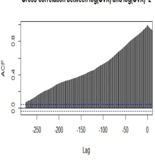
Furthermore, the cross-correlations are positive which means that an increase in the log-OVX today leads to an increase in the volatility of the log-log-OVX tomorrow; see Figure 3. This phenomenon is known as volatility feedback. It is quite often present in equity assets and can be part of the reason for the existence of an asymmetric response of oil volatility to oil price changes; see Wu (2001) for a helpful explanation of this phenomenon.
Table 2 reports the results of unit root and long memory tests. Different tests have been used. The first is the traditional Augmented Dickey-Fuller (ADF), whose null hypothesis is the existence of a unit root. The second is that proposed by Phillips and Perron (1988) (hereafter PP) whose null hypothesis coincides with that of the ADF test, but considers the possibility of existence of serial correlation and heteroskedasticity in the analyzed series. Regarding the long memory tests, we have used a modified version of the R/S test proposed by Lo (1991) and
a modified version of the V/S test proposed by Giraitis et al. (2000). In both tests the null hypothesis is that the process has short memory against the alternative that it has long memory. The difference is that the V/S test takes into consideration different lags. For choosing the lags we have used the Bayesian Information Criterion (BIC). The results of unit root tests suggest that log-OVX is stationary; see Table 2. Looking at the long memory test results, we observe that both reject the null of short memory which imply that log-OVX has long memory and can be modeled either by an ARFIMA or a HAR model; see Fernandes et al. (2014) for similar results regarding the log-VIX.
3. Long range dependence models
This section presents the models that coexist in the literature and proposes new extensions of the HAR model that include measures of oil asymmetry that take advantage of more refined ways of measuring the impact of oil price changes on the economy. The majority of the studies use the traditional dummy variable approach (e.g. Basher and Sadorsky, 2006; Nandha and Faff, 2008; Sadorsky, 2008). In this paper, we follow Hamilton (1996) and Ramos and Veiga (2011) that propose a measure that compares the current price of oil with the previous reference value. This measure is named NOPD and tries to capture the exogenous component of price variation. Besides, Lee et al. (1995) observe that in periods of turbulence the effects of oil price changes are smaller than in periods where oil prices are stable. In order to measure this properly they propose an asymmetric measure named SOPD.
3.1. The ARFIMA model
Given that the tests confirm the presence of long range dependence, we consider a well-known model that captures this feature of the data. The model is the autoregressive fractional integrated moving average model denoted ARFIMA(p,d,q) and is given by
Φ(L)(1−L)dyt= Θ(L)t for d∈(−0.5,0.5), (1)
where {t}Tt=1 is a white noise process with E(t) = 0 and variance σ2 and L is the lag operator
where Lyt=yt−1. The fractionally integrated order, d, is bounded to guarantee the stationarity
of the process. The polynomials Φ(L) = 1−φ1−...−φpLp and Θ(L) = 1−θ1L−....−θqLq have
orders p and q, respectively. Moreover, all their roots are outside the unit circle to guarantee the stationarity of the AR part and the invertibility of the MA process, respectively. Note that
Ut= (1−L)dyt is an ARM A(p, q) process.
3.2. The HAR model
Corsi (2009) asserts that the ARFIMA model fails to have a clear economic interpretation and it is not easy to estimate. For this reason, Corsi (2009) proposes the HAR model which is more interpretable and captures well the long range dependence of the volatility. It is described as an “additive cascade model” in which the actions of market participants are considered through the volatility components. By substituting the partial volatilities recursively, the model achieved with this process is autoregressive and its components are the volatility in specific time moments.
In this paper, we consider the following specification of the HAR model where the time horizons are daily, weekly, monthly and quarterly, that is, t= (1,5, 22, 66), respectively:
yt =φ0+φ1yt−1+φ5y¯t−1:5+φ22y¯t−1:22+φ66y¯t−1:66+εt, (2)
where yt =log-OVXt, ¯yt:i = 1i i−1 P j=0
yt−j and {εt}Tt=1 is a sequence of independent white noise
disturbances.
3.3. The HAR-Leverage model
Corsi et al. (2012) propose an extension of the HAR model by considering the asymmetric response of the volatility, that is, negative shocks have more impact on the volatility than positive shocks of the same magnitude. This effect is known in the literature as leverage. Therefore, the HARL includes, besides the traditional regressors of the HAR model, the negative oil returns at daily, weekly, monthly and quarterly frequency.2 The model is defined as
yt=β0+β1yt−1+β2y¯t−1:5+β3y¯t−1:22+β4y¯t−1:66+γ1r−t−1+γ2rt−−1:5+γ3rt−−1:22+γ4r−t−1:66+ε1t, (3)
where ¯yt:i is given as above, daily oil returns are defined asrt=pt−pt−1 withptbeing the price of
oil in logarithm at timetand past aggregated negative returns are given byrt−−1:t−h = h1(rt−1+...+ rt−h)I(rt−1+...+rt−h<0)withI{.}an indicator function that takes the value one if (rt−1+...+rt−h <0) and zero otherwise, and ε1t is defined asεt in equation (2). Some implementations of the model
for the high-frequency data of stock markets can be found in Chang and McAleer (2009), Louzis et al. (2012), Wang and Huang (2012) and Wang et al. (2015), among others.
3.4. The Net-HAR and Scaled-HAR models
In this subsection, we introduce two new extensions of the HAR model. The first includes the asymmetric measure NOPD while the second takes in consideration the SOPD. Before defining the models, we present the two oil asymmetric measures. The NOPD is defined as
N OP Dt=min[0,ln(oilt)−ln(max(oilt−1, ..., oilt−252))], (4)
where N OP Dt is the net price decrease at time t. NOPD can be interpreted as the extreme
negative returns over the last year.
The SOPD is different from the NOPD because its main aim is to measure how surprising is an oil price change decrease. It is known that an unexpected oil price change will have less impact when the volatility is high because it will be regarded as transitory. The SOPD is defined as
SOP Dt=min(0,ˆ∗t), (5)
2In a first step, we have also considered positive oil returns because an increase in oil prices will affect negatively
the economy and stock markets of oil importing countries. Note that oil is a global input. Therefore, positive oil price changes are considered bad news, and consequently, the asymmetry is expected to be of opposite direction than that found for equity; see Ramos and Veiga (2011, 2013) for some results on oil price shocks. However, these effects are stronger when we study the impact of oil price changes on stock markets and consequently, in this paper, we have considered that oil negative returns affect more the log-OVX.
where ˆ∗t is the oil standardized return at timet. The estimated conditional variance is obtained by fitting a Student-EGARCH(1,1) model to the daily oil returns. This model outperforms a set of benchmarks in term of goodness-of-fit according to the Akaike (AIC) and Bayesian information criterion (BIC).
Next, we convey the previous asymmetric measures by incorporating them into the HAR model instead of the conventional measures of asymmetry. This naturally suggests two extensions of the HARL model. The first is denoted the Net-HAR (N-HAR) model and is given by
yt = β00 +β10yt−1+β20y¯t−1:5+β30y¯t−1:22+β40y¯t−1:66 + γ10N OP Dt−1+γ20N OP Dt−1:5+γ30N OP Dt−1:22+γ40N OP Dt−1:66+ε2t, (6) where N OP Dt:i = 1i i−1 P j=0
N OP Dt−j, while the second extension is named Scaled-HAR (S-HAR)
and is given by
yt = β000+β 00
1yt−1+β200y¯t−1:5+β300y¯t−1:22+β400y¯t−1:66
+ γ001SOP Dt−1+γ200SOP Dt−1:5+γ300SOP Dt−1:22+γ400SOP Dt−1:66+ε3t,
(7)
where SOP Dt:i = 1i i−1 P j=0
SOP Dt−j, and, as before, {ε2t}tT=1 and {ε3t}Tt=1 are sequences of
inde-pendent white noise errors.
4. Empirical results
The aim of this section is to analyze the in and out-sample performances of the models presented in Section 3. The in-sample analysis consists in fitting the models to the log-OVX and study their goodness-of-fit while the out-of-sample analysis consists in forecasting the log-OVX one-day-ahead and analyze the results with predictive ability and Generalized-AutoContouR tests.
4.1. In-sample results
In this subsection, we fit the new asymmetric extensions of the HAR model and benchmarks to the series of log-OVX. We only present the estimates of the ARFIMA models that have been selected as the best among their homologous according to the AIC criterion.
Table 3 reports the estimation results of the ARFIMA model obtained using the OX package named ARFIMA. The results show that the estimate of the long memory parameter,d, is quite close to 0.5 and statistically significant, meaning that there is a strong long range dependence in the log-OVX series. Furthermore, the autoregressive parameter is itself of high magnitude. Its value is 0.868 which also suggests the existence of high persistence.
Table 4 reports the estimates of the HAR model and its extensions. All HAR-type models are estimated using OLS. Regarding the estimation of the HAR model, we observed that all frequencies of the aggregate log-OVX are statistically significant except that corresponding to the quarter. In particular, the log-OVX depends strongly on the previous day and month.
Regarding the estimation of the specifications with leverage we observe that monthly and quarter oil negative returns are statistically insignificant at 5% and 1% significance level, respec-tively. The estimated signs of the coefficients are negative which means that negative returns
affect positively the volatility of oil, as it was expected. Regarding the new extensions we observe that NOPD is only statistically significant at 10% significance level for the 22-day frequency while SOPD is significant at 1-day frequency. The adjustedR2s are very similar among the HAR-type
models while the log-likelihoods reveal that the HARL fit the log-OVX slightly better. The model with the worst fit is the N-HAR.
Finally, we compute the autocorrelations of squared residuals of order one, ten and one hundred for the HAR-type models and we observe that they are statistically significant which indicates the presence of heteroscedasticity in the residuals. Consequently, we extend the previous HAR models by including conditional heteroscedasticity and estimate HAR-type models given by (2), (3), (6) and (7) withεit and i= 0,1,2,3
εit =σtzt
σ2t =ω0+ω1εit2−1+ω2σt2−1,
(8) where zt follows the Hansen (1994)’s skew Student(v, λ) distribution with v corresponding to
the degrees of freedom and λ to the skewness.3 Furthermore, ω0 > 0, ω1 ≥ 0 and ω2 ≥ 0 to
guarantee the positiveness of the conditional variance andω1+ω2 <1 to assure the stationarity
of the process.
The HAR-GARCH-skewStudent-type models are estimated by maximum likelihood. The full estimation results appear in Table 5. We observe that the parameters of the conditional variance are statistically significant for all HAR-GARCH-skewStudent-type models and that the log-likelihoods increase substantially, suggesting an important increase in the goodness-of-fit of the models. Note that the best model in terms of log-likelihood is now the N-HAR-GARCH-skewStudent, although the likelihoods are quite similar for all models. Regarding the asymmetric effects, we observe that they are almost not significant with the exception of the 66-day negative return in the HARL-GARCH-skewStudent model.
Finally, comparing the results of Tables 3–5, we can observe that the model with the best fit in terms of log-likehood is the ARFIMA.
In the next subsection, we proceed to analyze the forecasting performance of the models with the best log-likelihood values.
4.2. Forecasting results
This section focuses on the forecasting of the log-OVX one-step-ahead. We have used a fixed rolling window scheme with 1000 observations. In total, for all models, we have 1339 one-step-ahead out-of-sample forecasts.
The models’ forecasting performance is evaluated using either the MCS procedure by Hansen et al. (2011) and programmed in R by Catania and Bernardi (2015) and the G-ACR test proposed by Gonz´alez-Rivera and Sun (2015). Hansen et al. (2011)’s procedure consists of a sequence of statistic tests to construct a set of models called “Superior Set Model” (SSM). Models in the SSM have statistically the same predictive ability, and they are ranked by the value of the loss function. The test statistic is calculated for an arbitrary loss function and evaluates point forecasts. On
3We have also tried the normal-inverse Gaussian distribution (NIG) as suggested by Corsi et al. (2008) but
models’ goodness-of-fit decreased and we have chosen to use the skew Student distribution of Hansen (1994) instead. Results are available by the authors upon request.
the other hand, the G-ACR test has as aim to evaluate the adequacy of the conditional forecast density model based on the probability integral transforms (PITs). It has as advantage the possibility of obtaining a graph named “autocontour” based on the PITs that may indicate the reason for the failure of the model.
4.3. Point forecasts
Table 6 displays the SSM of the log-OVX forecasting models under study. The loss functions are the squared error (SE) that is defined as (log-OVXt+1 −log-OVX\t+1)2 and the QLIKE of Patton (2011) that is a robust loss function to the presence of noise in the volatility proxy and it is defined asQLIKE ≡ log-OVXt+1
\
log-OVXt+1−log
log-OVXt+1 \
log-OVXt+1−1. The results depend on the loss function. When the SE loss function is used, only one model is in the SSM at 95% confidence level. The model is the N-GARCH-skewStudent. When the QLIKE loss function is used the HAR-GARCH-skewStudent, N-HAR-GARCH-skewStudent and S-HAR-GARCH-skewStudent have a similar predictive ability at 95% and 80% confidence levels. Yet, the models that are always ranked first under the two loss functions are the N-HAR-GARCH-skewStudent or/and the S-HAR-GARCH-skewStudent. The ARFIMA model is always excluded from the SSM although it is the best model in terms of goodness-of-fit.
4.4. Density forecasts
In this subsection, we use the G-ACR test of Gonz´alez-Rivera and Sun (2015) that is based on PITs. The test is based on the idea that if the proposed conditional density forecast coincides with the true one (H0), then the sequence of PITs {ut}Ht=1, where H is the total number of
one-step-ahead forecasts, must be i.i.dU(0,1).
The PITs can be plotted in the plane (ut, ut−k) such that the square with
√
αi-side and origin
at (0,0) contains αi% of observations, that is:
G-ACRk,αi ={B(ut, ut−k)⊂ < 2|0≤u t≤ √ αi and 0≤ut−k≤ √ αi, s.t.:ut×ut−k≤αi}. (9)
The proportion of PITs inside the cube defined in (9) is given by
b αk,i = H P t=k+1 Ik,αi t H−k , where Ik,αi
t is an indicator that takes value one if (ut, ut−k) ∈ G-ACRk,αi and zero otherwise. Therefore, the test statistic is given by
tk,αi =
b
αk,i−αi
σαi
,
where σαi is obtained by bootstrap. Note that this statistic is asymptotically standard normal distributed under the null hypothesis. Moreover, it is constructed for a single fixed autocontour,
αi, and a single fixed lag,k. But, we can go further and use a test statistic that considers a set of
lags with a fixed autocontour. In this case, considerLαi = (`1,αi, ..., `K,αi)
`k,αi =αbk,i−αi. Under the null hypothesis L 0 αiΛ −1 αiLαi is asymptotically χ 2 K distributed, where
Λαi is the asymptotic variance covariance matrix. Finally, we can also consider a test statistic for several autocontours with a fixed lag. Let Ck be a vector such that Ck = (ck,1, ..., ck,C)0 with
ck,i = αbk,i−αi. The test statistic is C 0 kΩ
−1
k Ck, where Ωk is the asymptotic variance covariance
matrix. The test statistic follows asymptotically aχ2C distribution (see Gonz´alez-Rivera and Sun, 2015, for details on these test statistics).
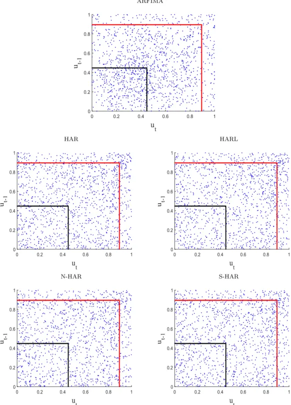
Figure 4 plots the PITs calculated for the selected models. For the ARFIMA model we observe a concentration of points in the middle of the graph, suggesting that the conditional forecast densities of the ARFIMA model are misspecified if Gaussian errors and conditional homoscedasticity are assumed. On the other hand, the PITs of the HAR-type models are more uniformed distributed but still a bit concentrated in the area of the right upper corner, suggesting that the conditional forecast densities constructed by the proposed models are not fitting well the true one-step-ahead forecast densities (see Mazzeu et al., 2017, for the interpretability of this graphical tool). One possibility to investigate in the future is the use of more flexible distributions for the errors of all models.
Table 7 reports the results of the test statistics presented above. We have implemented a parametric bootstrap procedure for approximating the asymptotic variance and covariance matrix of the tests in order to take into account the parameter uncertainty as suggested by Gonz´alez-Rivera and Sun (2015). Given that the estimation of the ARFIMA model and the bootstrap procedure for calculating the asymptotic variance is too demanding computationally, we only provide the results of the tests for the HAR-GARCH-type tests. This decision does not affect the evaluation of the ARFIMA model since from Figure 4, we observe that it performs worse than the competitors. The benefit of the tests is to distinguish among the HAR-GARCH-type models. Therefore, we compute the proportions αbk,i, for k = 1, ...,5 and 13 autocontours.
Looking at the table, we observe that the coverages are below the nominal levels for the middle autocontours. Regarding the individualt1,αi statistics, we also observe that the null hypothesis is rejected mainly for the middle autocontours and the number of rejections increase if we consider the portmanteau statistic L5
αi, being the HAR-GARCH-skewStudent the most rejected model while the S-HAR-GARCH-skewStudent is the least rejected for the significance levels of 5% and 1%. Finally, regarding the portmanteau C13
1 statistic, only the HAR-GARCH-skewStudent and
N-HAR-GARCH-skewStudent models are rejected.
All in all, the scale HAR-GARCH with errors following a skew Student distribution seems to do a good job in forecasting the log-OVX one-step-ahead.
5. Conclusion
This paper examines the time-series properties of the crude oil ETF volatility index at the daily frequency. Our study shows that it has a similar dependence structure as the CBOE’s market volatility index, i.e, it is stationary but its autocorrelation function decays hyperbolically towards zero, which implies that the index displays long range dependence typically captured either by fractional integrated autoregressive models or by heterogeneous autoregressive specifications.
Regarding the HAR-type models, we have considered the pure HAR model and its asymmetric version named HAR leverage as benchmark models and have proposed two new extensions that consider oil net and scaled measures of oil price changes instead of negative returns for modeling
the asymmetry. The first has as aim to measure how unsettling a decrease in the price of oil is likely to be for the spending decisions of consumers and firms while the second intends to measure how surprising an oil price decrease is for the observed oil price changes. Note that an unexpected oil price change will have less of an impact when conditional variances are high because much of the change in oil prices will be regarded as transitory. We have also considered a flexible distribution for the errors.
The out-of-sample forecasting analysis shows that, in terms of point forecasts, the models that forecast better the logarithm of the crude oil ETF volatility index are the HAR-GARCH and the two new asymmetric extensions of the HAR-GARCH model. In fact, these models have a similar predictive ability. Regarding density forecasting, the best model is the one that includes the scaled measure.
All in all, the results confirm that the inclusion of these new measures of oil asymmetry improves both the goodness-of-fit of models and considerably their forecasting performance.
Tables and figures
Figure 1. Daily OVX (left) and log-OVX (right) from May 5, 2007 till April 17, 2017.
Table 1
Descriptive statistics
Sample statistics (mean, standard deviation, skewness, kurtosis) and tests of normality for the log-OVX. p-values in (parenthesis). Sample statistics Mean 3.558 Standard Deviation 0.357 Skewness 0.091 Kurtosis 3.100
Jarque & Bera 4.559 (0.992)
Figure 2. Sample autocorrelation function of the log-OVX.
Table 2
Unit root and long memory tests
The table reports the statistics of different unit root and long memory tests: ADF, PP, modified R/S and modified V/S. The values in (parenthesis) for the V/S are the number of lags considered. The third column provides the tests’ critical values at a 5% significance level.
Test Test statistic 5% critical value
ADF -3.070 -2.860 PP -2.870 -2.860 R/S 2.190 1.860 V/S 7.570 (2) 1.360 4.570 (5) 2.11 (10) Table 3 ARFIMA–Estimation results
The table reports the estimation of the parameters together with the standard errors in (parenthesis) and the log-likelihood (LL) at the optimum.***,**,* means significance at 1%, 5% and 10%, respec-tively. Parameters Estimates d 0.493∗∗∗ (0.010) φ 0.868∗∗∗ (0.017) θ -0.471∗∗∗ 0.032 LL 4001.0
Table 4
HAR-type models estimation
The table reports the estimates of parameters together with the standard errors in (parenthesis), theR2, the log-likelihood (LL)
at the optimum, the correlations of squared residuals of order
k (ρ2
k) and the p-values of the Ljung-Box type test statistic in (parenthesis).***,**,* means significance at 1%, 5% and 10%, respectively.
HAR HARL N-HAR S-HAR Intercept 0.026∗∗∗ 0.045∗∗∗ 0.026∗ 0.041∗∗∗ (0.011) (0.011) (0.014) (0.014) log-OVX 1-day 0.911∗∗∗ 0.893∗∗∗ 0.889∗∗∗ 0.892∗∗∗ (0.020) (0.022) (0.022) (0.022) log-OVX 5-days 0.050∗ 0.051∗ 0.057∗∗∗ 0.066∗∗∗ (0.026) (0.027) (0.029) (0.027) log-OVX 22-days 0.041∗∗ 0.031 0.041∗∗ 0.038∗∗ (0.019) (0.021) (0.022) (0.020) log-OVX 66 days -0.009 0.011 0.006 -0.004∗∗ (0.010) (0.012) (0.013) (0.002) 1-day (-) return -0.083 (0.075) 5-day (-) return 0.108 (0.190) 22-day (-) return -0.968∗∗ (0.473) 66-day (-) return -1.125∗ (0.654) NOPD 1-day -0.048 (0.040) NOPD 5-days 0.002 (0.051) NOPD 22-days 0.054∗ (0.033) NOPD 66-days 0.008 (0.016) SOPD 1-day -0.004∗∗ (0.002) SOPD 5-days -0.001 (0.004) SOPD 22-days 0.009 (0.007) SOPD 66-days -0.026 (0.020) R2 0.982 0.982 0.983 0.982 AdjustedR2 0.982 0.982 0.983 0.982 LL 3904.9 3914.9 3641.0 3907.8 Residuals ρ21 0.305 0.306 0.302 0.299 (0.000) (0.000) (0.000) (0.000) ρ2 10 0.040 0.041 0.039 0.038 (0.000) (0.000) (0.000) (0.000) ρ2 100 -0.013 -0.013 -0.015 -0.013 (0.000) (0.000) (0.000) (0.000)
Table 5
HAR-GARCH-skewStudent-type models estimation The table reports the estimates of parameters together with the stan-dard errors in (parenthesis), the log-likelihood (LL) at the optimum, the correlations of squared residuals of orderk(ρ2
k) and the
correspond-ing p-values computed by the corrected test of Li and Mak (1994) in (parenthesis). ***,**,* means significance at 1%, 5% and 10%, respec-tively.
HAR HARL N-HAR S-HAR
Conditional mean Intercept 0.013 0.013 0.010 0.012 (0.008) (0.010) (0.011) (0.009) log-OVX 1-day 0.940∗∗∗ 0.940∗∗∗ 0.939∗∗∗ 0.932∗∗∗ (0.020) (0.024) (0.021) (0.023) log-OVX 5-days 0.014 0.011 0.004 0.019 (0.025) (0.029) (0.026) (0.027) log-OVX 22-days 0.047∗∗∗ 0.052∗∗∗ 0.055∗∗∗ 0.043∗∗∗ (0.016) (0.018) (0.018) (0.016) log-OVX 66 days -0.004 -0.008 -0.001 0.002 (0.009) (0.011) (0.011) (0.010) 1-day (-) return -0.024 (0.073) 5-day (-) return 0.107 (0.180) 22-day (-) return -0.475 (0.358) 66-day (-) return 0.921∗∗ (0.382) NOPD 1-day 0.007 (0.034) NOPD 5-days -0.043 (0.042) NOPD 22-days 0.041 (0.026) NOPD 66-days -0.004 (0.012) SOPD 1-day -0.002 (0.002) SOPD 5-days 0.002 (0.004) SOPD 22-days -0.005 (0.009) SOPD 66-days -0.012 (0.017) Conditional variance ω0 0.000∗∗∗ 0.000∗∗∗ 0.000∗∗∗ 0.000∗∗∗ (0.000) (0.000) (0.000) (0.000) ω1 0.094∗∗∗ 0.092∗∗∗ 0.091∗∗∗ 0.093∗∗∗ (0.022) (0.027) (0.021) (0.021) ω2 0.805∗∗∗ 0.811∗∗∗ 0.807∗∗∗ 0.805∗∗∗ (0.045) (0.043) (0.044) (0.043) v 4.431∗∗∗ 4.429∗∗∗ 4.458∗∗∗ 4.412∗∗∗ (0.417) (0.413) (0.403) (0.376) λ 0.193∗∗∗ 0.194∗∗∗ 0.193∗∗∗ 0.192∗∗∗ (0.031) (0.036) (0.030) (0.028) LL 3976.1 3977.8 3978.2 3977.8 Residuals ρ2 2 0.004 0.004 0.004 0.005 (0.218) (0.201) (0.192) (0.216) ρ2 10 0.009 0.009 0.009 0.010 (0.857) (0.846) (0.845) (0.846) ρ2 100 -0.009 -0.009 -0.010 -0.008 (0.181) (0.190) (0.177) (0.218)
ARFIMA 0 0.2 0.4 0.6 0.8 1 ut 0 0.2 0.4 0.6 0.8 1 u t-1 HAR HARL 0 0.2 0.4 0.6 0.8 1 ut 0 0.2 0.4 0.6 0.8 1 u t-1 0 0.2 0.4 0.6 0.8 1 ut 0 0.2 0.4 0.6 0.8 1 u t-1 N-HAR S-HAR 0 0.2 0.4 0.6 0.8 1 ut 0 0.2 0.4 0.6 0.8 1 u t-1 0 0.2 0.4 0.6 0.8 1 ut 0 0.2 0.4 0.6 0.8 1 u t-1
Figure 4. Pairs (ut, ut−1) and autocontours for the studied models. The PITS are obtained
assuming the errors follow either a Normal distribution (ARFIMA) or a skewed Student dis-tribution (HAR-type models); see Hansen (1994). ACR20%,1 corresponds to the black box and ACR80%,1 to the red box.
Table 6
Model confidence set results
The table reports the rankings of the log-OVX forecasters with different loss functions. – means that the model does not be-long to the MCS. The statistical tests are done at 95% and 80% confidence levels and 5000 bootstrap samples.
Models Loss functions
95% 80% SE QLIKE SE QLIKE ARFIMA – – – – HAR – 3 3 3 HARL – – – – N-HAR 1 2 1 2 S-HAR – 1 2 1 pvalue 0.746 0.996 0.845 0.998
T able 7: G-A CR test results The table rep orts the results of the G-A CR tests for the HAR-GAR CH-sk ewStuden t-t y p e mo dels fitted to log-O VX. Th e tests are computed assuming that the errors follo w the sk ew ed Studen t distribution; see Hansen (1994). *, **, *** indicat e that H0 is rejected at 10%, 5% and 1% lev els of significance, resp ectiv ely . HAR αi 0.01 0.05 0.1 0.2 0.3 0.4 0.5 0.6 0.7 0.8 0.9 0 .95 0.99 b α1 ,i 0.018 0.058 0.105 0.198 0.300 0.382 0.465 0.567 0.676 0.809 0.899 0 .952 0.993 | t1,α i | | 2 . 598 | ∗∗∗ | 1 . 180 | | 0 . 506 | | 0 . 132 | | 0 . 028 | | 1 . 055 | | 1 . 973 | ∗∗ | 1 . 928 | ∗ | 1 . 517 | | 0 . 642 | | 0 . 079 | | 0 . 257 | | 0 . 640 | L 5 αi 10 . 153 ∗ 6.040 12 . 905 ∗∗ 13 . 572 ∗∗ 12 . 912 ∗∗ 13 . 040 ∗∗ 13 . 554 ∗∗ 9.150 18 . 690 ∗∗∗ 19 . 644 ∗∗∗ 10 . 521 ∗ 1.844 0.444 C 13 1 21 . 778 ∗ HARL b α1 ,i 0.011 0.047 0.090 0.182 0.277 0.365 0.454 0.552 0.656 0.791 0.903 0 .943 0.993 | t1,α i | | 0 . 382 | | 0 . 398 | | 0 . 960 | | 1 . 320 | | 1 . 420 | | 1 . 993 | ∗∗ | 2 . 476 | ∗∗ | 2 . 680 | ∗∗∗ | 2 . 601 | ∗∗∗ | 0 . 612 | | 0 . 258 | | 0 . 821 | | 0 . 690 | L 5 αi 2.139 1.743 7.688 16 . 438 ∗∗∗ 20 . 402 ∗∗∗ 20 . 314 ∗∗∗ 14 . 433 ∗∗ 11 . 417 ∗∗ 16 . 270 ∗∗∗ 14 . 500 ∗∗ 5.448 6.453 0.518 C 13 1 17.548 N-HAR b α1 ,i 0.013 0.058 0.108 0.197 0.287 0.388 0.466 0.564 0.674 0.815 0.908 0 .951 0.993 | t1,α i | | 0 . 899 | | 1 . 159 | | 0 . 874 | | 0 . 201 | | 0 . 822 | | 0 . 728 | | 1 . 953 | ∗ | 2 . 075 | ∗∗ | 1 . 589 | | 1 . 087 | | 0 . 719 | | 0 . 083 | | 0 . 563 | L 5 αi 2.799 4.995 10 . 614 ∗ 12 . 963 ∗∗ 12 . 098 ∗∗ 20 . 891 ∗∗∗ 15 . 221 ∗∗∗ 12 . 109 ∗∗ 15 . 616 ∗∗∗ 12 . 082 ∗∗ 4.850 0.819 0.323 C 13 1 24 . 240 ∗∗ S-HAR bα 1 ,i 0.013 0.058 0.110 0.199 0.306 0.387 0.466 0.570 0.673 0.805 0.903 0 .951 0.993 | t1,α i | | 0 . 839 | | 1 . 123 | | 0 . 957 | | 0 . 082 | | 0 . 351 | | 0 . 711 | | 1 . 858 | ∗ | 1 . 710 | ∗ | 1 . 602 | | 0 . 330 | | 0 . 254 | | 0 . 083 | | 0 . 692 | L 5 αi 5.776 5.399 11 . 995 ∗∗ 6.825 15 . 119 ∗∗∗ 15 . 140 ∗∗∗ 12 . 083 ∗∗ 8.131 12 . 403 ∗∗ 9 . 500 ∗ 10 . 848 ∗ 3.993 0.505 C 13 1 16.574
References
Basher, S. A. and P. Sadorsky (2006). Oil price risk and emerging stock markets. Global Finance
Journal 17(2), 224–251.
Carr, P. and L. Wu (2006). A tale of two indices. Journal of Derivatives 13(3), 13–29.
Catania, L. and M. Bernardi (2015). MCS: Model Confidence Set Procedure. R package version 0.1.1.
Chang, C.-L. and M. McAleer (2009). Daily tourist arrivals, exchange rates and volatility for Korea and Taiwan. The Korean Economic Review 25(2), 241–267.
Chen, Y., K. He, and L. Yu (2015). The information content of OVX for crude oil returns analysis and risk measurement: Evidence from the Kalman filter model. Annals of Data Science 2(4), 471–487.
Clements, A. E. and J. Fuller (2012). Forecasting increases in the VIX: A time-varying long volatility hedge for equities. NCER Working Paper Series 88.
Corrado, C. J. and T. W. Miller, Jr. (2005). The forecast quality of CBOE implied volatility indexes. Journal of Futures Markets 25(4), 339–373.
Corsi, F. (2009). A simple approximate long-memory model of realized volatility. Journal of
Financial Econometrics 7(2), 174–196.
Corsi, F., F. Audrino, and R. Reno (2012). HAR modeling for realized volatility forecasting. In
Handbook of Volatility Models and Their Applications, pp. 363–382. New Jersey, USA: John
Wiley & Sons, Inc.
Corsi, F., S. Mittnik, C. Pigorsch, and U. Pigorsch (2008). The volatility of realized volatility.
Econometric Reviews 27(1-3), 46–78.
Fernandes, M., M. C. Medeiros, and M. Scharth (2014). Modeling and predicting the CBOE market volatility index. Journal of Banking & Finance 40, 1–10.
Fleming, J., B. Ostdiek, and R. E. Whaley (1995). Predicting stock market volatility: A new measure. Journal of Futures Markets 15(3), 265–302.
Giot, P. (2005). Implied volatility indexes and daily value at risk models. The Journal of Portfolio
Management 31(3), 92–100.
Giraitis, L., P. Kokoszka, R. Leipus, and G. Teyssi`ere (2000). Semiparametric estimation of the intensity of long memory in conditional heteroskedasticity. Statistical Inference for Stochastic
Processes 3(1), 113–128.
Gonz´alez-Rivera, G. and Y. Sun (2015). Generalized autocontours: Evaluation of multivariate density models. International Journal of Forecasting 31(3), 799–814.
Hamilton, J. D. (1996). This is what happened to the oil price-macroeconomy relationship.
Journal of Monetary Economics 38(2), 215–220.
Hansen, B. E. (1994). Autoregressive conditional density estimation. International Economic
Review 35, 705–730.
Hansen, P. R., A. Lunde, and J. M. Nason (2011). The model confidence set. Econometrica 79, 453–497.
Jiang, G. J. and Y. S. Tian (2005). The model-free implied volatility and its information content.
Review of Financial Studies 18(4), 1305–1342.
Konstantinidi, E., G. Skiadopoulos, and E. Tzagkaraki (2008). Can the evolution of implied volatility be forecasted? evidence from European and US implied volatility indices. Journal
of Banking & Finance 32(11), 2401–2411.
Lee, K., S. Ni, and R. A. Ratti (1995). Oil shocks and the macroeconomy: The role of price variability. The Energy Journal 16(4), 39–56.
Li, W. K. and T. K. Mak (1994). On the squared residual autocorrelations in non-linear time series with conditional heteroskedasticity. Journal of Time Series Analysis 15(6), 627–636. Lo, A. W. (1991). Long-term memory in stock market prices. Econometrica 59(5), 1279–1313. Lobato, I. N. and C. Velasco (2004). A simple test of normality for time series. Econometric
Theory 20(4), 671–689.
Louzis, D. P., S. Xanthopoulos-Sisinis, and A. P. Refenes (2012). Stock index realized volatility forecasting in the presence of heterogeneous leverage effects and long range dependence in the volatility of realized volatility. Applied Economics 44(27), 3533–3550.
Mazzeu, J., Gonz´alez-Rivera, E. Ruiz, and H. Veiga (2017). A bootstrap approach for generalized autocontour testing. Implications for VIX forecast densities. IDEAS, Working Paper.
Nandha, M. and R. Faff (2008). Does oil move equity prices? A global view. Energy
Eco-nomics 30(3), 986–997.
Patton, A. J. (2011). Volatility forecast comparison using imperfect volatility proxies. Journal
of Econometrics 160(1), 246–256.
Phillips, P. C. B. and P. Perron (1988). Testing for a unit root in time series regression.
Biometrika 75(2), 335–346.
Ramos, S. B. and H. Veiga (2011). Risk factors in oil and gas industry returns: International evidence. Energy Economics 33(3), 525–542.
Ramos, S. B. and H. Veiga (2013). Oil price asymmetric effects: Answering the puzzle in international stock markets. Energy Economics 38, 136–145.
Sadorsky, P. (2008). Assessing the impact of oil prices on firms of different sizes: Its tough being in the middle. Energy Policy 36(10), 3854–3861.
Simon, D. P. (2003). The Nasdaq volatility index during and after the bubble. The Journal of
Derivative 11(2), 9–24.
Wang, T. and Z. Huang (2012). The relationship between volatility and trading volume in the Chinese stock market: A volatility decomposition perspective. Annals of Economics and
Finance 13(1), 211–236.
Wang, X., C. Wu, and W. Xu (2015). Volatility forecasting: The role of lunch-break returns, overnight returns, trading volume and leverage effects. International Journal of
Forecast-ing 31(3), 609–619.
Whaley, R. E. (2000). The investor fear gauge. The Journal of Portfolio Management 26(3), 12–17.
Whaley, R. E. (2009). Understanding the VIX. The Journal of Portfolio Management 35(3), 98–105.
Wu, G. (2001). The determinants of asymmetric volatility. The Review of Financial