Asset Liability Management for Icelandic
Pension Funds
The Stochastic Programming Approach
by
Gísli Már Reynisson
in Partial Fulfillment of the Requirements for the Degree of
Mater of Science in Financial Economics
Thesis Supervisors:
Prof. Dr. Helgi Tómasson and Asst. Prof. Dr. Steinn Guðmundsson
Faculty of Economics
School of Social Science at University of Iceland February 2012
Asset Liability Management for Icelandic Pension Funds.
The Stochastic Programming Approach
This dissertation is in fulfillment of the requirements for the M.Sc. degree
in Financial Economics at the University of Iceland. The dissertation is
to the value of 30 ECTS credits. The M.Sc. degree requires 90 ECTS
credits.
School of Social Science at University of Iceland
c
2012 Gísli Már Reynisson
No part of this dissertation may be reproduced without the permission
of the author.
Printing: Prentlausnir ehf.
Reykjavik, 2012
Abstract
In this thesis a modeling framework to aid Icelandic pension funds in their asset allocation decisions is introduced. The framework is based on stochastic programming and asset liability management methodologies, where emphasis is placed on the uncertainty in the liabilities of the pension funds as well as the current Icelandic regulatory and supervisory environment.
The modeling framework is based on three interacting components: modeling the underlying stochastic variables; a scenario generator; and a stochastic programming model which is formulated as a multistage recourse problem in discrete state space and is solved with a scenario-based technique. Computational experiments presented in this thesis are carried out for a hypothetical pension fund, where market valued liabilities and premiums are used and the current capital controls are not accounted for.
The credibility of the model is analyzed in terms of in-sample stability and analysis on spurious changes in the optimized asset allocation. This vital attribute has received little attention in similar studies. The model performance is measured by comparison with partly dynamic fixed-mix investment strategies in terms of stronger actuarial position at the horizon. In addition, analysis of the most influential con-straints is carried out with sensitivity analysis.
The weakest component of the framework proved to be the scenario generator which was unable to generate a sufficient number of scenarios for satisfactory in-sample stability. In terms of performance and credibility, the model outperformed the partly dynamic fixed-mix benchmarks, in terms of stronger actuarial position at the horizon with no drastic changes in the optimal asset allocation. The most influential constraint is maximum allowed purchases in each year. Finally, comparison based on actuarial position, where liabilities and premiums are valued with fixed 3.5 percent interest rate, suggests that the interest rate risk is underestimated in the actuarial valuation methods currently used by the Icelandic Financial Supervisory Authority.
Preface
This dissertation is in fulfillment of the requirements for the M.Sc. degree in Financial Economics at the University of Iceland. The dissertation is to the value of 30 ECTS credits. The M.Sc. degree requires 90 ECTS credits. It is accomplished under the supervision of Prof. Dr. Helgi Tómasson and Asst. Prof. Dr. Steinn Guðmundsson. I would like to express my utmost gratitude for their support, guidance and construc-tive criticism during the writing of this dissertation.
I also would like to thank Eiríkur Dór Jónsson and Ólafur Örn Jónsson at Arion Bank for their professional opinions regarding real pension fund modeling as well as, providing me with necessary data.
Finally I would like to thank my family and friends for their support and encour-agement during the last weeks of writing.
Contents
Preface ii List of Notation iv List of Figures vi List of Tables ix 1 Introduction 31.1 The Asset liability management framework . . . 4
1.1.1 Modeling techniques . . . 5
1.1.2 Optimization under uncertainty . . . 6
1.2 Motivation . . . 8
1.3 Problem description . . . 8
1.4 Thesis structure . . . 9
2 The Icelandic pension system 11 2.1 Recent developments . . . 12
2.2 Actuarial position . . . 15
3 The Stochastic programming approach 19 3.1 General multistage recourse formulation . . . 20
3.2 Scenario based recourse formulation . . . 21
3.3 The asset liability model . . . 22
3.3.1 Constraints . . . 22
3.3.2 Objective function . . . 24
4 Scenario tree generation 26 4.1 Literature survey . . . 27 4.1.1 Sampling methods . . . 27 4.1.2 Statistical methods . . . 28 4.1.3 Probabilistic methods . . . 31 4.1.4 Other methods . . . 32 4.1.5 Scenario reduction . . . 33 4.2 Minimal requirements . . . 33
4.2.1 Stability and bias . . . 33
4.2.2 Arbitrage free scenario trees . . . 34
4.3.1 Notations for scenario trees . . . 35
4.3.2 K-means . . . 36
4.3.3 Modified K-mean clustering . . . 38
4.3.4 Extended K-means clustering . . . 39
4.4 Summary . . . 41
5 Modeling stochastic variables 42 5.1 Economic variables . . . 42
5.1.1 Inflation . . . 42
5.1.2 Exchange rate returns . . . 44
5.1.3 Yield curves . . . 45
5.1.4 Summary . . . 51
5.2 Liabilities and premiums . . . 51
5.2.1 Risk factors . . . 52
5.3 Modeling asset returns . . . 54
5.3.1 Return on cash and deposits . . . 54
5.3.2 Stock returns . . . 54 5.3.3 Bond returns . . . 59 6 Numerical results 61 6.1 Implementation . . . 61 6.2 Model setup . . . 62 6.3 Computational experiments . . . 63 6.3.1 In-sample stability . . . 67 6.3.2 Fixed-mix comparison . . . 72 6.3.3 Sensitivity analysis . . . 73
6.3.4 Fixed interest rate valuation . . . 77
7 Conclusions and future work 79 7.1 Conclusions . . . 79
7.2 Future work . . . 81
Appendix I 82
Appendix II 84
List of Notation
Stages (time periods) are denoted by an indextwith an initial stage denoted byt = 0
and and a final stage (the horizon) denoted by T. All stages considered are periods of one year, which is the time span from the time t−1 to timet.
Individual assets are denoted with an index j. The number of individual assets is denoted withJ. To ease the notation a little, isj also used to denote a stochastic variable. The distinction is however clear in context.
Asset classes are denoted by an index q. This is done to clearly separate asset classes from assets. The reason is that one asset class, foreign stocks, is composed of four stock indices.
In addition we have the frequently used notation
Sets
T: Set of times from the present to the horizon,T ={1,2, . . . , t, . . . , T}.
J: Set of stochastic variables,J ={1,2, . . . , j, . . . , J}.
N: Set of simulated paths, N ={1,2, . . . , n, . . . , N}.
S: Set of scenarios, S ={1,2, . . . , s, . . . , S}.
Q: Set of asset classes, Q={1,2, . . . , q, . . . , Q}.
Stochastic variables
ξj: Stochastic variable j.
ξtj: Stochastic process coherent with stochastic variablej,
˜
ξj : Simulated paths of stochastic variable j, ξˆj n ={ξ˜ j 1, . . . ,ξ˜ j N} ˜
ξnj(t): Value of the nth simulated path of stochastic variable j at staget.
The scenario tree
B: Branching structure, B={b1, . . . , bt, . . . , bT}.
C(t,s): Cluster at stage t in scenario s.
Co(t,s): The center of a cluster C(t,s)(its position)
ps: Unconditional probability that scenario s occurs.
rusd(t,s): Exchange rate returns in cluster C(t,s).
π(t,s): Inflation in clusterC(t,s).
spot(t,s): One year real yields in clusterC(t,s).
gm2,m1: A m2-to-m1 real yield spread. (m2 > m1).
qm2,m1: A m2-to-m1 nominal yield spread. (m2 > m1).
yr(t,s)(m): Real yield for maturity m inC(t,s).
yn(t,s)(m): Nominal yield for maturity m in C(t,s).
The Optimization Model
Decision variables
ht,j: Holdings in asset j at stage t, whereht,j ≥0.
pt,j: Purchase in asset j at a stage t, wherept,j ≥0.
st,j: Sales in asset j at a stage t, where st,j ≥0.
Ztarget: Penalty variable for funding ratios which do not reach the
pre-specified target funding ratio at the horizon.
Zmin: Penalty variable for funding ratios which fall below the pre-specified minimum ratio.
Wt: Wealth of the pension fund at stage t.
Stochastic variables
R(t,jt,s): Return on asset j at stage t in scenario s.
˜
Li: Present value of future liabilities of the pension fund at stage time t. ˜
Ii: Present value of premiums of the pension fund at stage time t.
Parameters
h0j: Initial holdings in assetj.
cj: Transaction cost for asset j.
lj: Lower bound (as a percentage of wealth) for holdings in asset j.
uj: Upper bound (as a percentage of wealth) for holdings in asset j
lq: Lower bound (as a percentage of wealth) for holdings in asset class q.
uq: Upper bound (as a percentage of wealth) for holdings in asset class q.
up: Upper limit (as a percentage of wealth) for purchase. FRtarget: Funding ratio of the pension fund at decision timet. FRmin: Funding ratio of the pension fund at decision timet.
List of Figures
1.1 Taxonomy of methods for optimization under uncertainty. . . 7
1.2 Interplay between the components of the multistage stochastic pro-gramming framework. . . 10
2.1 Yearly real return from end of year 2000 to end of year 2010. Source:
The Icelandic Financial Supervisory Autority,www.fme.is . . . 13
2.2 Historical asset allocation of Icelandic pension fund with the follow-ing legend. () Deposits, () domestic fixed income securities, () domestic variable income securities, () foreign variable income secu-rities and () other asset classes. Source: The Icelandic Financial Supervisory Authority, www.fme.is . . . 14
2.3 Assets as a share of GDP in % (fifteen highest ratios) at the end of year 2010. Source: OECD Global Pension Statistics,www.oecd.org 15
2.4 The structure of the total actuarial position. Source: (Baldvinsson, 2004, p. 53) . . . 16
4.1 Schematic representation of a scenario tree and a scenario fan. . . . 26
4.2 Schematic representation of a three stage scenario fan, composed of nine simulated paths, and a resulting scenario tree with branching structure B={1,3,2}. . . 36
5.1 Structure of the real yield curve simulation method, where (•) denotes spot yield and () denotes real yields y(t,s)(m), m={5,10,15,20}. . 48
5.2 Eight simulated real yield curves (dashed lines) and Arion Banks av-erage real yield curve (solid line). Simulated yields, yr(t,s)(m) for m =
{5,10, . . . ,25}as well as spot yields are dented by ( ). . . 49 5.3 Structure of the nominal yield curve (solid line), the real yield curve
(dashed line) and their relation. . . 50
5.4 Dependencies between all models for the economic variables. . . 51
5.5 Pension fund actuarial position, measured with the funding ratio, val-ued for real interest rates ranging from 1% to 6%. . . 52
5.6 Historical prices of the five MSCI stock indices from 30 November 1981 to 30 November 2011. The starting values have been scaled to a value of 100 for comparison. Source: www.mscibarra.com . . . 57
5.7 Flowchart for generating asset returns, liabilities and premiums. Simu-lated inflation, real spot yields and stock prices realizations are bundled together into a scenario tree using the K-means clustering algorithm. The dotted box represents one cluster in the scenario tree. . . 60
6.1 Optimized asset allocation with the following legend. () Cash, () domestic stocks, () foreign stocks, () real bonds and () nominal bonds. . . 65
6.2 The efficient frontier for various pairs of the penalty parameters, (λ1, λ2). The black edged, red square corresponds to the solution. . . 65
6.3 Expected asset allocation for extreme pairs of penalty parameters, (λ1, λ2) with the following legend. () Cash, () domestic stocks, () foreign stocks, () real bonds and () nominal bonds. . . 66
6.4 The objective value for branching structures BS = {15, i,2} where
i= 2, . . . ,20. The solution is denoted by () . . . 67
6.5 Stability analysis on the three components of the objective value for branching structures BS={15, i,2} ,wherei= 2, . . . ,20. . . 68
6.6 Variability in the expected funding ratio, as a function of the risk aversion components, for BS = {15,7,2} (N) and BS = {15,15,2}
(). The solution is marked by red square with black edges. . . 69
6.7 Evolution of the expected wealth for seven scenario trees with BS =
{15,15,2}denoted by ( ) and the target wealth denoted by (N). The solution is denoted by (). . . 70
6.8 Expected asset allocation for the other six scenario trees, all with branching structure BS= {15,15,2}, with the following legend. () Cash, () domestic stocks, () foreign stocks, () real bonds and () nominal bonds . . . 71
6.9 Performance of the mulistage stochastic model compared to three bench-mark partly dynamic fixed-mix strategies, (%cash, % stocks, % bonds). 73
6.10 The effects, of altering the model parameters, on the expected funding ratio at the horizon. . . 74
6.11 The effects, of altering values on penalty parameters, on the expected asset allocation, with the following legend. () Cash, () domestic stocks, () foreign stocks, () real bonds and () nominal bonds. . 75
6.12 The effects, of altering values onFtarget, Fmin, up, on the expected asset
allocation with the following legend. () Cash, () domestic stocks, () foreign stocks, () real bonds and () nominal bonds. . . 76
6.13 Optimized asset allocation as a result of fixed valued (at 3.5%) liabili-ties and premiums. Panel (a) corresponds to penalty parameters (2,8), whereas panel (b) corresponds to the extreme case (∞,∞). E[WT]
figures in thousand ISK. () Cash, () domestic stocks, () foreign stocks, () real bonds and () nominal bonds. . . 77
7.1 Evolution of the modified K-means clustering method. . . 82
List of Tables
2.1 Accrued position, future position and total actuarial position for the ten largest pension funds and the Icelandic pension system at the end of year 2010. All figures in ISK thousand. Source: (Financial Supervisory Authority, 2011) . . . 17
2.2 Historical actuarial position, for all pension funds without guarantee, from end of year 2005 to end of year 2010. Source: Icelandic Financial Supervisory Authority (fme.is). . . 17
5.1 Estimated parameters for (5.1.1). Note that here the present state vari-ables are indexed with a zero rather thanT which might be misleading since they are estimated using the entire data series. This is however more convenient notation since the zero represents the beginning of the asset liability management study. . . 44
5.2 Estimates for CIR spot yield model (5.1.3), based on data provided by Arion Bank and three month REIBOR rates. . . 47
5.3 The shape and the scale parameters of the gamma spread distributions as well as the mean and the variance. . . 48
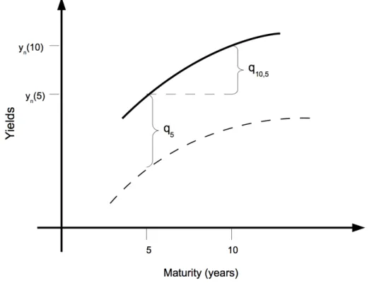
5.4 The scale, shape parameters as well as the mean and variance of the real-nominal spread distribution (q5) and the ten-to-five year nominal yield spread distribution (q10,5). . . 50 5.5 Historical average returns and volatility of five MSCI indices based on
monthly returns from 30 November 1981 to 30 November 2011. Yearly returns are estimated, by assuming normality, as µyear = 12µmonthly
and σyearly=
√
5.6 Historical estimated correlations, from 30 November 1981 to 30
Novem-ber 2011 . . . 58
5.7 Estimated parameters and standard errors (in brackets) in the DCC(1,1)-GARCH(1,1)model for five MSCI world indices based on historical prices from 30 November 1981 to 30 November 2011 usingccgarch pack-age for the statistical software R (www.r-project.org/) (Nakatani, 2009). . . 58
6.1 Scenario tree structure in six published asset liability management studies for pension funds. . . 62
6.2 Scenario tree structure, restriction and model parameters. . . 63
6.3 Breakdown of the computational time (in seconds) . . . 64
Chapter 1.
Introduction
In a world where financial markets have become seemingly increasingly complicated and more volatile, the need for professional financial management is becoming vital for a standard of living. As a result of a rise in life expectancy, pension funds are essential to ensure decent retirement years. From that perspective, individuals rely on pension fund managers to responsibly invest their contributions and they expect fair pension payments in return when they retire. Faced with the fact that financial crises have occurred fairly frequently the necessity for responsible allocation decisions made by pension fund managers are greater than ever. These decisions are made with respect to portfolio management theory as well as market experience. Rapid developments have taken place in the field of portfolio management and a vast number of sophisticated tools have emerged to aid managers in their decisions. Moreover, growing awareness of the importance of transparency, trust and fiduciary responsibility in portfolio management have led to a change in the attitude of pension funds managers toward their responsibilities.
Maginn et al. (2007) define portfolio management as a process which applies to all types of portfolio investments. They suggest that the process is based on an integrated set of steps undertaken in a consistent manner to create and maintain appropriate combinations of investment assets. The steps are
1. The planing step
2. Identifying and specifying the investors objectives and constraints 3. Creating investment policy statements
4. Forming Capital Market Expectations 5. Creating the Strategic Asset Allocation
Briefly stated, the planing step is governed by the specifications of investor, market and economic related input factors which are incorporated into the investor’s ob-jectives and constraints. The investment policy statement serves as a document for all investment decision making, which includes for example performance measures and guidelines for rebalancing. In the Capital market expectations step, long term
forecasts of risk and return measures are established. These forecasts serve as bench-marks for the strategic asset allocation decision (SAA) which is the final step. SAA lists the percentage of wealth invested in each asset class (portfolio policy) and is integrated with long term capital market expectations.
By itself, SAA can be defined as a process1 with certain well-defined steps, the
objective of which is to define the portfolio policy. Another type of asset allocations is tactical asset allocation (TAA), which deals with short term adjustments of the portfolio policy. For example, a pension fund’s SAA might state that it is coherent with the fund’s objective and risk aversion to hold 60% of its wealth in domestic government bonds. If at any time, the actual proportions held in this asset class drifts away, say to 55%, it is referred to as a tactical decision. The portfolio policy is often stated both in terms of SAA and TAA. In such a format, SAA are expressed as the target holdings in each asset class whereas TAA define the tolerance of deviation from the SAA. This gives the pension fund manager the flexibility of adjusting the portfolio according to his beliefs while staying within the limits of the portfolio policy. Defining portfolio management as a process emphasizes the fact that it requires constant consideration and revision through feedback. The process is centered around the the investment policy statement (IPS), and the necessity for feedback and main-tenance are vital features of the process. The IPS serves as the governing document for all investment decision making. Icelandic pension funds are bound by law2 to create and accompany the IPS which is kept at the forefront in the event of a dispute between the fund and its members.
1.1
The Asset liability management framework
In recent years, Icelandic pension fund managers have shifted the focus from return objectives, such as reaching a pre-specified average return over a few years, to in-tegrated asset and liability objectives, such as minimizing the risk of reduction in pension payments (Ó. Ö. Jónsson and E.D. Jónsson, personal interview, June 24, 2011). Such objectives generally concentrate on the asset-liability ratio, also known as the funding ratio. This shift in focus results in different risk measures. Before, the main risk factor was the uncertainty or the volatility of asset returns, as apposed to liability risk measures. The latter being a result of the integrated asset liability objectives. This growing awareness of the interplay between assets and liabilities is 1The definition of SAA varies in the litereture. One can either think of SAA as an individual
process inherent in portfolio management or as the result of the portfolio management process itself.
2Article 20 of Act 129/1997.
more consistent with the fundamental purpose of the pension system, which is to provide pension and disability payments to retirees as well compensation to spouses and children.
Consider the following example which further illustrates the necessity for an integrated view of assets and liabilities, in terms of interest rate risk. Suppose that a pension fund portfolio of assets has a duration of eight years and the fund is faced with future liabilities with duration of twenty five years. If yields decrease by one percent, then the asset portfolio increases by roughly eight percent and the liabilities increase by twenty five percent3. A Focus on return objectives, where only the asset side is
considered, results in overconfidence since the asset-liability ratio has decreased. The pension fund investment policy must take into account the interplay between the asset and the liability sides and this has given rise to the asset liability framework. In this framework, more emphasis is paid to balancing the asset and liability sides which results in increased awareness of other risk factors. Asset liability management studies are not only relevant for pension fund applications, but also for a wide range of applications where one is faced with future liabilities, e.g. insurance companies.
1.1.1
Modeling techniques
In general, all pension funds reinvest their collected premiums and pay old age pensions as well as compensation. However each, pension fund is unique. Apart from the different types of pension funds each fund is a reflection of its members. The age composition of the pension fund members’ has a great impact on the fund. Young members typically prefer more aggressive investment strategies and have a higher risk tolerance, whereas members closer to retirement are more concerned with risk of reduction in pension payments and generally prefer more conservative investment strategy. Also each pension fund is subject to preferences, beliefs and investment guidelines imposed by the fund’s manager and its board of directors. Moreover the ability to predict future liabilities is subject to the age compositions of the fund’s member. Such predictions are essential in asset liability management. This variability between pension funds requires a custom-designed model for each fund, where objectives and risk preferences can be modeled in sufficient detail.
A number of modeling methods and techniques have been suggested in the asset liability management literature. Frequently used methods in pension fund applica-tions are simulation and optimization under uncertainty. A fundamental difference
3Based on the first term taylor expansion,(∆Price)/Price=
is that in simulation, the portfolio policy is an input, which corresponds to static decision making. In optimization under uncertainty, the portfolio policy is the result, and the method allows for dynamic decision making. In addition Klein Haneveld, W.K., Streutker, M.H., van der Vlerk, M.H (2010) argue that optimization under uncertainty provides suitable and flexible framework in terms of incorporating nu-merous restrictions.
A study by Fabozzi, F.J. and Focardi, S.M. and Jonas, C.L. (2005) on 28 pension funds in four countries reveals that two thirds of the participating funds used opti-mization but many funds still prefer simulation over optiopti-mization, the main reason being that optimization models are time consuming and hard to implement.
1.1.2
Optimization under uncertainty
Optimization addresses the problem of finding a decision, often is subject to some constraints, that minimizes (or maximizes) a function. Using matrix notation, this is represented mathematically as min x f(x) subject to gi(x) = 0 , i= 1, . . . , n hj(x)≤0 , j =n+ 1, . . . , m (1.1.1)
where x, f(x) are referred to as decision variable(s) and the objective function and
gi(x), hj(x) are constraints. In general, optimization models are classified according
to the nature of the objective function and constraints. For example, when the objective function and all constraints are linear, problem (1.1.1) is referred to as a linear optimization problem.
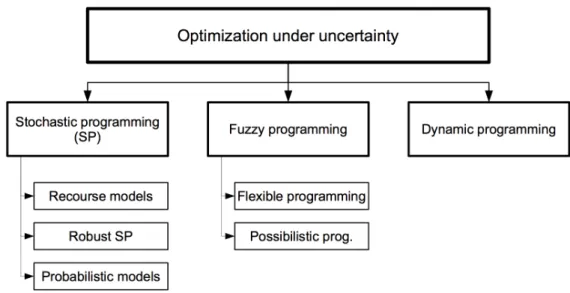
The problem of optimal decision-making in face of uncertainty is referred to as optimization under uncertainty. Optimization problems that include uncertainty have been applied in many fields, such as production planning, transportation, scheduling and finance to name a few. Uncertainty governs for instance the availability of raw materials in production planning, the demand for goods or the return of assets. In such problems, the objective function and/or constraints are represented as functions of stochastic variable(s), either discrete or continuous. Over the years a number of modeling philosophies and approaches have been suggested to cope with the complexity of such optimization problems. Three main methods are schematically
laid out in figure (1.1).
Figure 1.1. Taxonomy of methods for optimization under uncertainty.
The main methods differ on how the uncertainty is modeled. A sensible discussion of the different aspects of each method requires detailed formulations as well as numerous definitions and concepts, especially in the case of fuzzy programming. Instead the interested reader is referred to a comprehensive discussion and extensive survey presented by Sahinidis (2004). It is worth mentioning that publications in the literature governed by fuzzy programming for financial applications are scarce. The choice is therefore mostly between dynamic and stochastic programming.
In this thesis, the stochastic programming method is used for the following two main reasons. Asset liability management applications for pension funds presented in the literature are highly concentrated on stochastic programming4, e.g. see surveys
in Sodhi (2005); Ziemba & Mulvey (1998) or Zenios & Ziemba (2007). In addition a class of stochastic programming models can be reformulated into a large scale linear optimization problem. This is highly desirable since linear optimization problems are well studied and powerful solution methods exists.
4A number of applications presented in the literature are titled dynamic stochastic programming.
This is to emphasize that stochastic programming in general is dynamic, rather than dynamic programming is being used, which might be misleading.
1.2
Motivation
The collapse of the financial markets in late 2008 left many Icelandic pension funds severely underfunded in terms of their actuarial position5. Many funds are running a
high deficit and only two funds out of 24 showed a positive actuarial position at the end of year 2010 (Financial Supervisory Authority, 2011). This has forced Icelandic pension funds to reduce accrued pension rights. In late 2011 the fund Stapi was forced to make a staggering six percent reduction in accrued pension rights from contributions prior to 2010,6 and in the same year, a two point five percent reduction was made by the fund Almenni lífeyrissjóðurinn7.
A study by Frank J. Fabozzi & Jonas (2005) revealed that 90% of the private-sector defined-benefit pension plans in the UK and US were underfunded. The reason mostly bad modeling or the absence of modeling, together with difficult conditions in the financial markets. Although one cannot assume that this was the case for all the Icelandic pension funds and the current crisis, this issue is worth investigating further.
Tower Perrin-Tillinghast constructed an asset liability management system using a stochastic programming model to aid its pension plan clients, described in Mulvey et al. (2000). In the same paper, savings of USD 450 to USD 1,000 million in opportunity costs in US WEST’s pension plan was reported. Another example of successful application in asset liability management using stochastic programming is the Russell-Yasuda Kasai model. It was designed for Japanese insurance company and savings of USD 79 million was reported during the models first two years in use (Carino et al. , 1994). Although such large scale successes are rarely reported in academic papers, this increases the confidence that such modeling systems could prove very useful.
1.3
Problem description
Pension fund managers are concerned with the issue of forming an investment strategy which benefits the funds. More precisely, how should a pension fund allocate its wealth among the different asset classes such that the risk of reduction in pension payments is minimized?
5Discussed in more detail in section [2.2] 6The funds news report:
http://www.stapi.is/is/news/rettindi-laekka-um-6-/
7Specification was conditional on actuarial position at the end of year 2010 and are laid out in
The focus of this thesis is to introduce an alternative modeling framework based on stochastic programming. Its purpose is to aid a pension fund manager their asset allocation decisions. The model is based on asset liability management methodology, which is ideal for pension funds and on stochastic programming which is adjusted to the environment in which Icelandic pension funds operate. In addition, emphasis is placed on taking the current regulatory and supervisory constraints into account to make the model as realistic as possible.
Several models, based on asset liability management studies from a stochastic programming point of view, are available in the literature. However each model has to be custom designed according to the pension funds at hand. Specifications in terms of objectives and risk aversion of the fund, as well as the regulatory framework, must be incorporated into each model.
Little attention has been paid to the quality of asset allocation decisions suggested by the models in the literature. This aspect will be investigated in this thesis by analyzing the stability of the solution, as well as the effects of individual model parameters on the solution. Furthermore, an important question which has not received much attention in the literature is whether the resulting asset allocation decisions are realistic. In this thesis credibility of the asset allocations will be analyzed in terms of spurious asset allocation switching between time periods. This is essential if the model is to be used in practice. The performance of the model introduced in this thesis is measured by comparison with partly dynamic fixed-mix investment strategies in terms of stronger actuarial position at the horizon. The term fixed-mix applies to constant portfolio rebalancing to maintain fixed holdings in each asset class. The strategies are partly dynamic in the sense that although holdings in each asset class are fixed, no additional restrictions are placed on holdings in individual assets.
1.4
Thesis structure
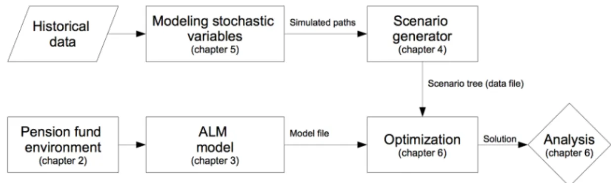
The model introduced in this thesis is based on the following three interacting components:
1. Modeling the underlying stochastic variables 2. Scenario generation
3. A multistage optimization model
Each part is covered in detail in separate chapters, along with a brief description of the Icelandic pension system. The interplay between the three parts is shown in
figure 1.2, where references to relevant chapters are shown in brackets.
Figure 1.2. Interplay between the components of the multistage stochastic program-ming framework.
Chapter 2.
The Icelandic pension
system
The present day pension system in Iceland dates back to the general wage settlement of the spring of 1969, a result of negotiations between the State, labour unions and the Federation of Icelandic Employers. In the beginning of 1970 the labor unions traded a wage increase for the setting up of a fully funded mandatory occupational pension fund which is the dominant feature of today’s Icelandic pension system. The occupational pension funds became general in 1970, then mandatory by law for wage earners in 1974 and were extended to the self employed in 1980. A Law was adopted in 1991 on the annual accounts and auditing of pension funds (V. Árnason, 2010). This gave the Bank Inspectorate of the Central Bank of Iceland some supervisory role over the pension funds. A comprehensive reform took place in 1997 and 1998 which resulted in the current Pension act, Mandatory Guarantee of Pension Rights and the Operations of Pension Funds. This adoption proved difficult, in fact the work on legislation framework on pension funds had started in 1976 (Guðmundsson, 2001). The reform affected the mandatory occupational pension funds as well as introduction of tax incentives for voluntary individual pension savings. Since then, minor changes in the pension fund legislation have been imposed.
The current Icelandic pension system is based on three pillars. The First pillar is the Icelandic Social Security, generally referred to as the public pension system. It is a tax financed pension scheme which aims to secure each individual minimum pension payments which are reduced in relation to other income. It provides an old age pension along with survivor’s and disability pension. The public pension is divided into a basic pension and supplementary pension, both are paid from the age of 67. The Second pillar is a mandatory occupational pension scheme. It is mandatory by law1 to pay at least 12% of all wages and salaries from the age of 16, which is split between a 4% contribution from the employee and a 8% contribution
from the employer. According to Icelandic Law2 pension funds must pay a minimum coverage of 56% of monthly wages for 40 years of work. Occupational pension schemes are managed by private, fully funded, pension funds governed jointly by unions and employers and provide lifelong retirement and disability pension as well as pension to children and spouses. The majority of pension funds in the Second pillar are based on a defined contribution scheme without guarantee by the Treasury and Municipal Authorities. However, a few funds are based on defined benefit schemes with an employer guarantee. The Second pillar is the dominant feature of the Icelandic pension system. The funds are monitored by the Icelandic Financial Supervisory Authority3. The Third pillar forms a voluntary individual pension saving scheme
with tax incentives. The maximum deduction by the employee is 4% and in wage settlements employers have agreed to contribute 2% to these voluntary pensions if the employee matches the amount with at least the same percentage, making the maximum total contribution of 6%. The voluntary pension savings are in most cases a defined contribution pension scheme with individual accounts, where pension savings have to be paid in equal payments over of at least seven years from the age of 60 (Jónsdóttir, 2007). At the end of year 2010 the voluntary pension saving scheme accounted for 15.5% of the whole pension system (Financial Supervisory Authority, 2010).
2.1
Recent developments
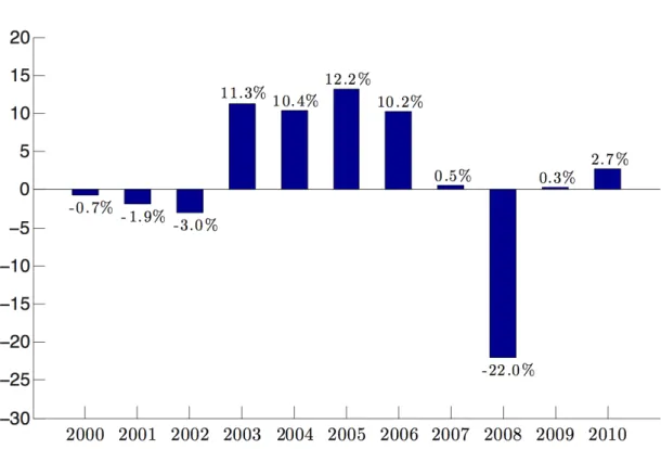
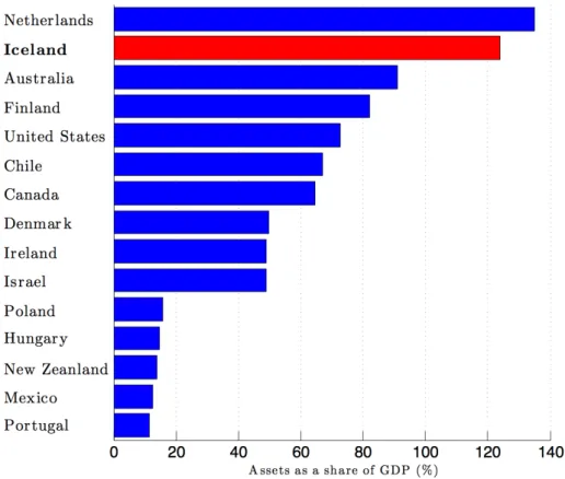
The Icelandic pension system has grown dramatically in the past 20 to 30 years. At end of year 2010 net assets amounted to roughly ISK 2,021 billion compared to ISK 522 billion at the end of 2000. The pension funds’ net assets as a share of gross domestic product (GDP) were 123.91% compared to 83.97% in 2001 and 11.6% in 1986. The growth is largely due to the advantageous age composition of the Icelandic nation and relative young age of the system, which results in positive cash flow in the system. Furthermore, indexation gave pension funds unusually good returns in the early years of the system. The pension system is dominated by a few large pension funds. At the end of year 2010, the three largest pension funds accounted for 47.2% of the pension system assets and the assets of the ten largest pension funds accounted for 80.1% of the whole pension system, (Financial Supervisory Authority, 2011). The Pension funds’ real return, accounted for inflation, was 2.65% at the end of year 2010 compared with 0.34% at the end of year 2009. Figure 2.1 shows the yearly real return
2Article 4 of Act 129/1997 3
from 2000.
Figure 2.1. Yearly real return from end of year 2000 to end of year 2010. Source:
The Icelandic Financial Supervisory Autority, www.fme.is
In the spring of 2008, pension funds managers realized that difficulties in the Icelandic economy were severe, particularly when the Currency Market collapsed in the spring. The fear became a reality when the Icelandic commercial banks fell in October of the same year. The pension funds, which had invested heavily in the Icelandic Financial sector, lost their shares in the three banks and had to depreciate much of the bank’s bonds. The collapse was not only tied to the financial sector, the entire domestic stock market plunged. The value of domestic stocks in pension fund portfolios were estimated at nearly ISK 24 billion at end of year 2008, compared to ISK 141 billion in September of the same year. Similarly the Icelandic bond market took a big downswing, particularly corporate bonds. Corporate bonds accounted for ISK 144 billion in pension funds portfolios in late December 2008, compared to ISK 189 billion in September. In 2008 the Icelandic krona fell by 80.24% and the average inflation was 16.34% (Óskarsdóttir, 2011). This led to a negative real increase of 22% of the pension funds’ net assets in 2008 as shown in figure 2.1.
Since the collapse, foreign exchange transactions have been subjected to capital controls, requested by the International Monetary Fund (IMF). Therefore new foreign investments are not allowed, and pension funds can only reinvest their wealth which was present before the controls. Together with the collapse of the domestic stock
market, investment opportunities are limited. Therefore pension funds increased their shares in government and housing bonds as well as deposits relative to previous years as shown in figure 2.2.
Figure 2.2. Historical asset allocation of Icelandic pension fund with the following legend. () Deposits, () domestic fixed income securities, () domestic variable income securities, () foreign variable income securities and () other asset classes. Source: The Icelandic Financial Supervisory Authority, www.fme.is
According to a study conducted by the Organisation for Economic Co-operation and Development (OECD) on pension funds’ assets as a share of GDP, Iceland’s pension system is large in comparison to the OECD nations at the end of year 2010 as shown in figure 2.3.
It is evident that many challenges await the Icelandic pension system in the near future. The liberation of the capital controls are in motion (Central Bank of Iceland, 2011), and the Icelandic stock market is just a fraction of its previous size. Until it regain some of its former size, investment opportunities are limited. On the liability side, changes in the age composition of the Icelandic nation and a possible increase in disability pension payments will affect the funds’ financial position. This requires that the funds invest their wealth responsibly to be able to cover future liability payments.
Figure 2.3. Assets as a share of GDP in % (fifteen highest ratios) at the end of year 2010. Source: OECD Global Pension Statistics,www.oecd.org
2.2
Actuarial position
In July each year Icelandic pension funds conduct an actuarial survey within the Mutual Insurance Division of the pension funds, as requested by the Icelandic Finan-cial Supervisory Authority. The actuarial survey is pursuant to the principal feature (article 24) of Act 129/1997 on the Mandatory Guarantee of Pension Rights and the Operations of Pension Funds, which took effect on 1 July 1998.
Pension funds liabilities are pension payments to retirees, disability pensions as well as compensations to spouses and children in case of the passing of a fund member. Premiums are paid contributions by fund members as mandated by law. Pension fund liabilities consist of accrued liabilities and future liabilities. Accrued liabilities are based promised on pension payments on already paid premiums. Future liabilities are estimated present values of liabilities which correspond to premium payments in the future. The estimates are based according to the articles of association of each pension fund and are based on members who contributed to the fund in the previous year. Future premiums are estimated present value of future contributions from active
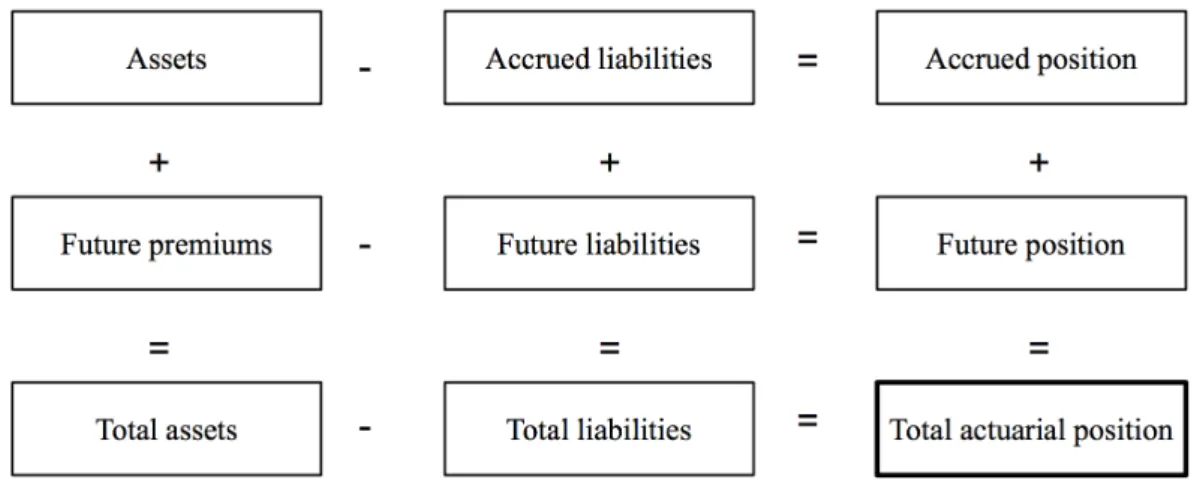
pension fund members. Figure 2.4 shows the structure of the total actuarial position4 which is used as an indicator to measure the funds’ ability to meet its liabilities.
Figure 2.4. The structure of the total actuarial position. Source: (Baldvinsson, 2004, p. 53)
Accrued position is thus calculated as the difference between assets and liabilities, and future position is calculated as estimated present value of future premiums less estimated present value of future liabilities. The total actuarial position is based on the sum of assets and future premiums less accrued and future liabilities (Financial Supervisory Authority, 2010). Table 2.1 shows the accrued position, future position and total actuarial position for ten largest pension funds as well as for the Icelandic pension system at the end of year 2010. In all cases, the accrued and total actuarial position is negative.
4The provisions of the 39th Article of Act 129/1997 about actuarial position only take into
Table 2.1. Accrued position, future position and total actuarial position for the ten largest pension funds and the Icelandic pension system at the end of year 2010. All figures in ISK thousand. Source: (Financial Supervisory Authority, 2011)
Pension fund Accrued Future Total actuarial
position postion position (in ISK) Lífeyrissjóður starfsmanna ríkisins -324,654 -73,159 -397,813
Lífeyrissjóður verslunarmanna -7,924 -12,009 -19,933 Gildi lífeyrissjóður -25,929 -10,366 -36,295 Stapi lífeyrissjóður -17,917 -6,242 -24,159 Sameinaði lífeyrissjóðurinn -11,097 787 -10,310 Almenni lífeyrissjóðurinn -6,868 1,406 -5,462 Frjálsi lífeyrissjóðurinn -4,275 472 -3,803 Stafir lífeyrissjóður -16,733 4,558 -12,175 Söfnunarsjóður lífeyrisréttinda -1,709 -1,571 -3,280 Festa lífeyrissjóður -6,507 -3,184 -9,697
Icelandic pension system -524,171 -127,465 -651,637
The total actuarial position (in %) is the ratio between total assets less total liabilities divided by total liabilities. Total assets are the sum of assets and future premiums and total liabilities are the sum of accrued and future liabilities. If the ratio is positive then the net assets at each time are sufficient to cover already promised liability payments which indicate strong actuarial position. According to article 39 of Act 129/1997, all pension funds without a guarantee, showing deficit of 10% or higher in a single year or a deficit higher than 5% for five consecutive years, must amend their Articles of Association in order to achieve a satisfactory actuarial position. In late December 2008, a transitional provision was added which uthorized pension funds to run a deficit up to 15% based on actual valuation for the year 2008, without making changes to the Articles of Association of the fund (Financial Supervisory Authority, 2009). Historical actuarial position for all pension funds without an employer guarantee is shown in table 2.2 from the year 2005 to 2009.
Table 2.2. Historical actuarial position, for all pension funds without guarantee, from end of year 2005 to end of year 2010. Source: Icelandic Financial Supervisory Authority (fme.is).
2005 2006 2007 2008 2009 2010 Positive 22 25 22 3 3 2 Deficit between 0,1% - 5% 12 8 4 7 3 8 Deficit between 5,1% -10% 3 2 3 7 6 10 Deficit between 10,1% - 15% 1 0 0 8 13 4 Deficit in excess of 15% - - - 4 3 0 Total: 38 35 29 29 28 24
The effects of the financial crisis on the actuarial position is evident. Prior to the crisis the majority of funds had a positive actuarial position, but after the crisis many funds showed a high deficit. Almost all funds with a guarantee from the Treasury and Municipal Authorities show a high deficit at the end of 2010. The highest deficit amounts to a staggering 99.3% which is however guaranteed (Financial Supervisory Authority, 2011).
Chapter 3.
The Stochastic
programming approach
The Committee on Stochastic Programming (COSP) (2011) describes, stochastic programming as a framework for modeling optimization problems that involve uncer-tainty. Stochastic programming models allow for progressive revelation of information in time and multiple decision stages, where each decision is adapted to the available information (Kouwenberg & Vorst, 1998). It is a general framework for modeling optimization problems that involve uncertainty. Several different methods for formu-lation exists for stochastic problems.
First explanations on the important concepts of stochastic programming is given. Stages correspond to the time periods when decisions are made and the horizon refers to the number of stages. It is assumed that at any stage, finitely many states of the system exist, and the states are described by (multidimensional) state variables. In stochastic programming the state variables are affected by uncertainty. Given the initial state of the system, the overall objective is to maximize (or minimize) some objective function of an immediate return for all stages and states, (Kall & Wallace, 1994).
Stochastic programming systems can be categorized, based on how information is reveled through time, (Yuet al. , 2003). In ananticipative formulation, also referred to as a static model, the decision does not depend in any way on future observations of the environment. In anAdaptive formulation, information related to the uncertainty becomes partially available before the decision making, so optimization takes place in a learning environment. The recourse formulation combines the former two models in a common mathematical framework, which seeks a policy that not only anticipates future observations but also takes into account temporarily available information to make recourse decisions.
For financial application, the recourse formulation is the most relevant. For exam-ple a portfolio manager considers both future movements of stock prices (anticipation) as well as the rebalancing of the portfolio as prices change (adaptation).
3.1
General multistage recourse formulation
In this thesis we consider a stochastic programming problem in the form of a multi-stage recourse problem in discrete multi-stage and state space, following (Dupačová, 1999; Kall & Wallace, 1994; Shapiro et al. , 2009).
Suppose there are T ≥ 2 discrete stages and that the uncertainty is expressed by the (multidimensional) random variable ξ1, . . . , ξT, which is revealed gradually
over time during the T stages. The decision process x1, . . . , xT is adapted to the
revelations of the random variables and has the form
decision realization · · · decision realization
(x1) (ξ2) (xT) (ξT)
The sequence ξt, for t = 1, . . . , T is viewed as a stochastic process1. Let ξbtc := (ξ1, . . . , ξt) denote the history of the process up to time t. At the first stage, the
state of the system is known and the outcome of the decision completely depends on the future realizations of the underlying stochastic process. Thereafter, for each realization of the historyξbtc up to time t, a recourse decision is made which is only allowed to be a function of the observed realizations (xbt−1c, ξbtc). In other words, the recourse decisions depend on the current state of the system as determined by previous decisions (xbt−1c) and by the information (ξbtc) available up to time t but not future observations. This adaption to the available information is the basic requirement for nonanticipativity, which will be discussed further later on.
The generic form of a T stage stochastic programming model can be written in nested formulation as min x1∈X1 f1(x1) +E inf x2∈X2(x1,ξ2) f2(x2, ξ2) +E · · ·+E inf xT∈XT(xT−1,ξT) fT(xT, ξT) (3.1.1) whereEis the expectation operator, the functionf1 :Rn1 →R and the setX1 ⊂Rnt are deterministic,xt∈Rnt,t= 1, . . . , T are decision variables andft :Rn1×Rm1 →R
are continuous functions fort = 2, . . . , T. For a linear multistage stochastic program we have
ft(xt, ξt) := cTtxt t= 2, . . . , T
X1 :={x1 :A1x1 =b1, x1 ≥0}
Xt(xt−1, ξt) :={xt:B1xt−1+Atxt =bt, xt≥0} t= 2, . . . , T
whereξ1 := (c1, A1, b1)is known and ξt:= (ct, Bt, At, bt)∈Rmt,t= 2, . . . , T are data
vectors or matrixes, whose elements are random.
The problem can be reformulated to (3.1.2), if the decision variables at timet are a function of the (data) process up to time t, xt=xt(ξbtc), t= 1, . . . , T
min x1,x2,...,xT E f1(x1) +f2(xt(ξb2c), ξ2) +· · ·+fT(xT(ξbTc), ξT) Subject to x1 ∈ X1, xt(ξbtc)∈ Xt(xt−1(ξbt−1c), ξt), t = 2, . . . , T. (3.1.2)
This formulation is often used in the stochastic programming literature. However unless the data process, ξ1, . . . , ξT, has a finite number of realizations, formulation
(3.1.2) leads to an infinite dimensional optimization problem (Shapiroet al. , 2009). In the case of discrete stages and a discrete states, one assumes that the proba-bility distribution of ξ is a discrete and is concentrated at a finite number of points. In such a case, the stochastic process is conveniently represented as a scenario tree.
3.2
Scenario based recourse formulation
For a discrete time state a scenario based formulation is a standard solution tech-nique. An alternative approach is to assume a continuous time stage, which leads to distribution-based solution techniques. In scenario based stochastic programming one assumes that the finite number of realizations of the stochastic process,ξ1, . . . , ξT,
is concentrated on a finite number of points, denoted ξ1, . . . , ξ,S.
This allows for a derivation of a deterministic equivalent formulation on the form
min x1,...,xT S X s=1 ps[f1(xs1) +f2(xs2) +f3(xs3) +· · ·+fT(xsT)] s.t A1x1 =b1 Bs 2x1 + As2xs2 =b2 Bs 3x2 + As3xs3 =b3 . .. . .. ... Bs TxT−1 + AsTxsT =bT (3.2.1) l≤xst ≤u t= 1, . . . , T s= 1, . . . , S
where ps denotes the probability of scenario s. In problem (3.2.1) all parts of the decision vector are allowed to depend on all parts of the random data. However, as previously discussed, decision xt made in stage t, should only be allowed to depend
constraints on the form
xbtic=xbtlc, for all i and l where ξbic,s =ξblc,s, t = 1, . . . , T (3.2.2) are included. Problem (3.2.1) together with the nonanticipativity constraints (3.2.2) are equivalent to the original formulation (3.1.1).
The term scenario tree might seem somewhat mysterious at this point, but this will be described in detail in the next chapter.
3.3
The asset liability model
The asset liability management model is formulated as an linear multistage stochastic problem. We assume that at the beginning (t = 0) the asset allocation for the next years is already determined. That is the asset portfolio is not optimized at the beginning of the study. Most of the constraints are standard in asset liability management studies and the notation follows (Hilli et al. , 2007) for most parts.
Before the model is presented three sets must be defined. Let J denote a set of assets where and T denote the set of discrete stages when decisions are made. However sometimes it is more relevant to express the constraints in terms of asset classes rather than individual assets. To that end let,Qdenote the set of asset classes considered. The model will be introduced in terms of constraints and a objective function.
3.3.1
Constraints
Inventory constraints
Inventory constraints describe holdings, purchases and sales of each asset over time. The inventory constraint at staget >0 are
ht,j =ht−1,j(1 +Rt,j) +pt,j −st,j, j ∈ J, t >0
whereRt,j denotes (random) return on assetj in stagetandht,j,pt,j,st,j are decision
variables, which describe the holdings, purchases and sales in asset j at stage t
respectively. The initial holdings in each asset are denoted by h0
j and are assumed to
Budget constraints
Budget constraints describe the cash inflow (revenues) and cash outflow (expenses) of the pension fund and ensure that the cash inflow never exceed the cash outflow. At stage t= 0 (precent) the budget constraints are
X j∈J (1 +cq)p0,j = X j∈J (1−cq)s0,j and at staget >0 X j∈J (1 +cj)pt,j +Lt= X j∈J (1−cj)st,j +It
where cj denotes the transaction cost for purchase and sales of asset class j, Lt
denotes the liability payments to pensioners and It denotes the premiums paid by
the pension fund’s members. The transaction costs are assumed to be equal for purchase and sales.
Portfolio constraints
Upper and lower limits of holdings in various asset classes for Icelandic pension funds are bound both by law and by the funds’ investment policy. Those limits are expressed as a proportion of the total wealth of the pension fund
lqX j∈J ht,j ≤ht,q ≤uq X j∈J ht,j, q∈ Q, t ∈ T
where the parameterslqand uq denote the upper and lower bounds for different asset
classes, and are assumed to be constant. Similar constraints are placed on holdings in foreign investments. To prevent spurious asset switching, the maximum amount allowed for purchase, as a percentage of the wealth, is introduced in stage t
pt,j ≤up J
X
j=1
ht,j, j ∈ J, t ∈ T
where the constant up denotes the maximum holdings (percentage). The wealth at
time t is given by
Wt=Wt−1+
X
j∈J
(1 +Rj,t)ht,j−1, j ∈ J, t ∈ T where W0 is the funds initial wealth.
Nonanticipativity constraints
Nonanticipativity constraints ensure that groups of scenarios2 with identical values
of the uncertain parameters in stagetmust yield the same decision up to that period. Letxbtsc denote a decision variable in scenarios from the precent (t = 0) up to stage
t. The nonanticipativity constraints can be expressed mathematically as
ht,jbsc =ht,jbs0c, pbt,jsc=pbt,js0c, st,jbsc =sbt,js0c
for scenarios s and s0 inheriting an identical past up to staget.
3.3.2
Objective function
The objective of the pension fund is to obtain a pre-specified target funding ratio at the end of the horizon. The funding ratio3 is denoted byF R
t and given by FRt= Wt−I˜t ˜ Lt −1 (3.3.1)
whereL˜tandI˜tdenote present value of future liability and premiums respectively. To
model the pension fund risk aversion, two penalty functions are introduced. First the objective is penalized for a funding ratio which falls below a pre-specified minimum, denoted FRmin. Secondly the objective is penalized for a funding which does note reach the target, FRtargetat the horizon. Both penalty functions consists of a constant multiplied with the first downward moment of the funding ratio. The two penalty constraints are obtained by rewriting equation (3.3.1) and introducing two positive decision variables, Ztarget and Zmin, i.e.
(WT + ˜IT)≥(1 +FRtarget) ˜LT −ZTtarget, Z target T ≥0 (WT + ˜IT)≥(1 +FRmin) ˜LT −ZTmin, Z min T ≥0.
If the funding ratio falls below the minimum or does not reach the target at the horizon, Ztarget and Zmin become positive. Since the deterministic equivalent formu-lation is based on a number of scenarios the expected funding ratio is maximized and penalized of the expected downside moments (times a constant) of the funding ratio.
2Scenarios are defined in chapter [4].
3The term funding ratio is similar to the total actuarial position (in %). However, the term
funding ratio is used in this thesis to emphasize that they differ in terms of valuation of future liabilities and premiums. This will be discussed in detail in chapter 5.
The the objective function becomes max E " WT + ˜IT ˜ LT −1 ! −λ1 ZTtarget ˜ LT −λ2 T X t=1 Zmin t ˜ Lt #
where λ1 and λ2 are the respective penalty constants. The two penalty components are strictly positive and are therefore subtracted from the expected funding ratio at the horizon. Similar penalty functions could be presented in terms of target wealth and or deviation from a specified target wealth.
An alternative way to model the risk aversion is to use chance constraints. Such constraints state that the funding ratio should at all times be higher than a pre-specified minimum value withhigh probability,
P
n
(Wt+ ˜It)≥(1 +FRmin) ˜Lt
o
≥α.
Chance constraints have a more intuitive appeal than penalty constraints. Moreover the reliability constant,α, is easier to determine than the penalty constantsλ1andλ2. However change constraints are computationally much more inefficient and complex. When included in the model, one has two options: Firstly one can make distributional assumptions to reformulate the chance constraints. However, few distributions will lead to convex and well behaved constraints. In the case of the normal distribution, the variance-covariance matrix for the different assets has to be estimated, which a non-trivial task. The second option is to reformulate the chance constraints into a mixed-integer or integrated change constraints, which need special algorithms and are generally harder to solve. This approach is described in detail in (Dert, 1995; Drijver, 2005; Klein Haneveld et al. , 2010).
Chapter 4.
Scenario tree generation
In this chapter important aspects of scenario tree generation are discussed and the scenario generation method used in this thesis introduced. The resulting scenario tree is used as input to the scenario based multistage recourse formulation of the stochastic programming model.
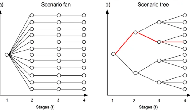
Before reviewing the scenario tree generation methods in the literature let’s address two important concepts, a scenario fan and a scenario tree which are shown in figure (4.1).
Figure 4.1. Schematic representation of a scenario tree and a scenario fan.
A scenario tree consists of clusters1 (marked with circles) and branches linking the
clusters together (marked as black/red lines). The rightmost cluster represents the present and is referred to as the root cluster, whereas the leftmost clusters represent the horizon and are referred to as the leaf clusters. A scenario is defined as a route from the root cluster to one of the leaf clusters. Each cluster has a one-to one
relation to certain staget and certain scenario s, denoted by(t, s). In a scenario fan, all clusters at stage t are connected to one cluster at stage t−1 and one cluster at stage t+ 1. In a scenario tree, bt−1 clusters at time t are connected to one cluster at time t−1 and branch of to bt+1 clusters at stage t+ 1. For example in figure 4.1, a pair of clusters at stage two are connected to one cluster at stage one and each cluster at stage two branches off to three clusters at stage three.
It is commonly understood that a scenario fan is only suitable in two-stage scenario based stochastic problems. A Two-stage problem might seem misleading since the scenario fan in figure 4.1 is represented by four stages. However the dependancies between clusters at stage two, three and four are the same. Therefore the scenario fan is argued to only adequately represent two stages, one and four in the figure (Sutiene & Pranevicius, 2007). In the case of a multistage scenario based on stochastic programming, a scenario tree is needed to represent the relation between clusters for all stages. The necessary notation for scenario trees is introduced in section 4.3.1.
The rest of this chapter is organized as follows. In section 4.1 the vast number of scenario generation methods in the literature is briefly introduced and discussed. In section 4.3 the scenario generator used in this thesis is explained in detail.
4.1
Literature survey
Scenario tree generation is not an easy task and a numerous methods have been suggested in the literature. The methods reviewed in this thesis can be classified into roughly four classes: sampling methods; statistical methods; methods based on probability or approximation theory and; other methods. In addition, a closely related subject of scenario reduction methods is briefly introduced.
4.1.1
Sampling methods
Various sampling methods can be used to construct the scenario tree. The simplest method is to sample randomly from historical data, known in the financial litera-ture as bootstrapping. Although easy to implement, it is seldom used in practical application due to its limitations. The main limitation of bootstrapping is that it is unable to generate samples different from those that already have occurred in the past. Therefore using bootstrapping to generate scenarios assumes that historical data is representative of the future and only identical observations can be resampled.
This means, for example, that more extreme values than observed from historical data are not available.
To overcome the drawbacks of bootstrapping, (Kouwenberg, 2001) suggests ran-dom sampling and adjusted ranran-dom sampling methods. The resulting scenario trees are used to solve an asset liability management model for a Dutch pension fund, where a vector autoregressive time series model (VAR) was used to estimate the stochastic parameters in the model. A random sampling method is based on sampling from the error distribution of the estimated VAR model. An adjusted random sampling method is based on antithetic sampling in order to fit every odd moment of the underlying distribution of the stochastic parameters by assuming an even number of clusters in the scenario tree. This method is based on one of the scenario generating methods considered in (Carino et al. , 1994) where the mean and the variance of the underlying distribution are fitted with an adjusted random sampling scheme. Backtesting, with rolling horizon simulation, revealed that random sampling can lead to extensive asset mix and spurious profits while the adjusted random sampling method led to less asset mixing and more stable solutions.
Dupačováet al. (2000) proposed a sequential sampling algorithm. This sampling method is an iterative algorithm which is part of a framework that uses a scenario tree nodal partition matrix, conditional sampling, stochastic programming generator and a solver. The scenario tree is modified through an update of the nodal partition matrix in each iteration and the stochastic programmin model solved. Another variation of a sampling algorithm discussed is based on the expected value of perfect information (EVPI). For further discussion see Dempster (1998); Dempster & Thompson (1999) and Heitsch & Römisch (2009) as well as their references.
Various Monte Carlo (MC) and Quasi Monte Carlo (QMC) sampling schemes have been considered in the literature. QMC methods have very good and well documented convergence properties and are therefore well suited for scenario gen-eration. QMC schemes that epi-converge to the original problem are presented in (Pennanen, 2005, 2009). MC based methods are presented in Chiralaksanakul (2003); Chiralaksanakul & Morton (2004).
4.1.2
Statistical methods
Moment matching
Arguably the most commonly used scenario tree generation method was initially introduced by Kouwenberg & Vorst (1998). The idea is to estimate the first two
moments of the underlying distribution in the scenario tree. This is obtained by solving small systems of the scenario tree recursively. The method was generalized by Høyland, K. and Wallace, S.W. (2001) and is known as the moment matching method. The moments and co-movements of the unknown distributions are matched with historical data or values pre-specified by the user. The matching is obtained by solving a non-linear optimization problem which penalizes deviation from the desired moments. The authors approximate the first four moments of the underlying distributions and the correlation between the assets. The resulting scenario tree is obtained by solving sequential non-linear optimization problems or by solving one large non-linear optimization problem. The computing time grows hand in hand with the size of the scenario tree and quickly becomes large when dealing with realistic problems. To overcome this problem, a somewhat successful attempt to decrease the solution times, by introducing a heuristic algorithm, was introduced in Høyland, K. and Kaut, M. and Wallace, S.W. (2003). Another suggestion, using parallel implementation, was proposed by Beraldiet al. (2010).
The main drawback to this method is that convergence to the optimal solution is not guaranteed. This means that the method may diverge, resulting in a spurious scenario tree. In addition, increasing the number of scenarios will not lead to a better match of the observed and desired moments. Another drawback, pointed out by Hochreiter & Pflug (2007), is that matching the first four moments of a distribution can result in many different distributions which have only the first four moments in common. For example, uniform and normal distribution may have the same four moments but have very different characteristics. Underlying distributions for financial data indicate unimodal features. Ji et al. (2005) point out that if only the first four moments are used to estimate the scenario tree, the resulting distribution may have a multimodal feature which is not representative of financial data. They argue therefore that descriptive features such as unimodality must be included in the moment matching procedure. This is achieved with partition of the distribution space of the stochastic parameters and imposing additional constraints in the moment matching optimization.
In financial applications, scenario trees should be free of arbitrage opportunities2. Klaassen (2002) demonstrates that the moment matching method does not strictly prevent arbitrage opportunities. To prevent arbitrage opportunities, two additional non-linear optimization problems must be solved at each node of the scenario tree to detect and prevent arbitrage. Those two non-linear optimization problems can also be added as constraints to the main moment matching model. Jiet al. (2005) modified
the moment matching method to prevent arbitrage opportunities by solving a linear optimization during every iteration of the sequential version of the moment matching method. The additional constraints mentioned above will increase the already high computing times.
In addition to the random sampling and adjusted random sampling methods, discussed previously, Kouwenberg (2001) also construct a scenario tree with the moment matching method. The performance, of those three methods, on the solution of the asset liability management model for the Dutch pension fund are analyzed. Kouwenberg reports that the moment matching method slightly outperformed the adjusted random sampling technique. A fixed-mix strategy was used as a benchmark for comparison. On the positive side the solution of the asset liability management model that used the moment matching scenario generation method was the only one whish strictly outperformed the fixed-mix benchmark.
Clustering
Another method proposed by Dupačová et al. (2000) is a multi-level clustering method. In general clustering methods consist of two phases, the simulation phase and the clustering phase. In the simulation phase, many different paths are simulated from the underlying time series model, where each simulated path represents one possible evolution of the future. All the simulated paths are generally referred to as a scenario fan. In the second phase the scenario fan is molded into a scenario tree by bundling together similar scenario paths into clusters at different points in time. Usu-ally the clustering method assumes that some time series models have been estimated beforehand. Simulated paths which are nearest to a cluster by some distance measure are assigned to each cluster. A similar approach is proposed by Gulpinaret al. (2004) where a randomized clustering algorithm is used in the clustering phase. Two methods are proposed for the simulation phase, parallel simulation and sequential simulation. In the parallel simulation, all paths are simulated before clustering begins whereas in the sequential simulation, the simulation phase and clustering phase are performed alternately until the whole scenario tree is completed. In more detail, a large number of paths are simulated and then bundled into so called first stage clusters. Then the simulation is initialized at each first stage cluster and new scenario fans are simulated which are then bundled together into second stage clusters. This is repeated until the scenario tree is completed. The difference between the two methods is that parallel simulation requires storage of large number of simulated paths whereas in sequential simulation only scenarios from the relevant clusters are stored at each